chapter #1 eee8013 linear controller design and state ... eee8013 -matlab.pdfchapter 1 eee8013...
TRANSCRIPT

Chapter 1 EEE8013
Module Leader: Dr Damian Giaouris – [email protected] 1/13
Chapter #1
EEE8013
Linear Controller Design and State Space Analysis
Using Matlab to Solve ODE

Chapter 1 EEE8013
Module Leader: Dr Damian Giaouris – [email protected] 2/13
1. First order ODEs
Introduction: In this part of the module, we will extensively use
Matlab/Simulink to enhance the material that we covered during the normal
lectures. As this part of the module is addressed only to MSc/MEng students,
it is anticipated that you will be prepared, you will have studied and
reproduced this material before you come to the lab, and hence these sessions
will only address problems that you faced, and cover extra material/examples.
I want to emphasize that these sessions in the computing lab are NOT normal
lectures, but are here only to help with your self-driven studies.
In the first chapter, we will see how we can find the numerical solution of
ODEs and how to simulate analytical solutions of ODEs. It is crucial to
understand the difference between numerical solution and simulation of the
analytical solution. Obviously both solutions must give you the same result.
Example:
𝑑𝑥
𝑑𝑡= −
6
5𝑥
Hence 𝑘 = −6
5 and 𝑢 = 0
Since k is negative the system is stable and the solution will converge to
zero (unforced system) starting from the initial condition 𝑥(0) = 1. The
analytical solution can be written as: 𝑥(𝑡) = 𝑒𝑘𝑡𝑥(0) = 𝑒−6
5𝑡
Now, we will numerically solve the given ODE:
System 1Choose different ICs
Numerical Solution
Analytical Solution
t-6/5t
exp(-6/5t)
Scope2
Scope1
Scope
Product1
Product
eu
Math
Function2
eu
Math
Function1
eu
Math
Function
1
s
Integrator1
1
s
Integrator
1
Gain6
-6/5
Gain5
1
Gain4
6/5
Gain3
-6/5
Gain2
6
Gain1
1/5
Gain
0
Constant1
0
Constant
Clock2
Clock1
Clock
x
x
u Dx
ax

Chapter 1 EEE8013
Module Leader: Dr Damian Giaouris – [email protected] 3/13
5𝑑𝑥
𝑑𝑡+ 6𝑥 = 0, 𝑥(0) = 1
This ODE can be written as:
5𝑑𝑥
𝑑𝑡= −6𝑥 + 0
Remember to include the initial condition 𝑥(0) = 1 by double clicking on
the integrator block and put 1 in “Initial condition”:
System 1Choose different ICs
Numerical Solution
Analytical Solution
Scope1
Scope
Product1
Product
eu
Math
Function1
eu
Math
Function
1
s
Integrator1
1
s
Integrator
1
Gain4
6/5
Gain3
-6/5
Gain2
6
Gain1
1/5
Gain
0/6
Constant1
0
Constant
Clock1
Clock
x
x
u Dx
ax

Chapter 1 EEE8013
Module Leader: Dr Damian Giaouris – [email protected] 4/13
To see the output x(t) double click on Scope:
Now you need to check that all scopes are showing the same result for x(t).
If I want to plot x(t) versus time in Matlab then select the Scope’s
parameters:
Select “History”:
Chapter 1 EEE8013
Module Leader: Dr Damian Giaouris – [email protected] 5/13
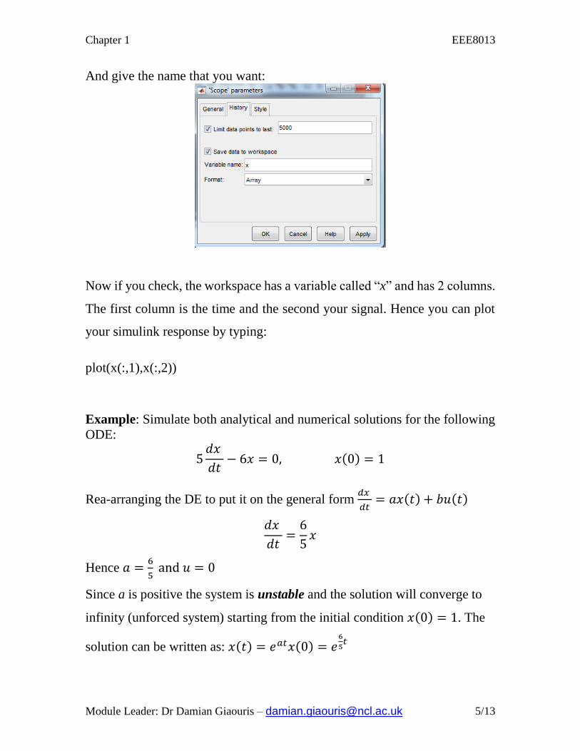
And give the name that you want:
Now if you check, the workspace has a variable called “x” and has 2 columns.
The first column is the time and the second your signal. Hence you can plot
your simulink response by typing:
plot(x(:,1),x(:,2))
Example: Simulate both analytical and numerical solutions for the following
ODE:
5𝑑𝑥
𝑑𝑡− 6𝑥 = 0, 𝑥(0) = 1
Rea-arranging the DE to put it on the general form 𝑑𝑥
𝑑𝑡= 𝑎𝑥(𝑡) + 𝑏𝑢(𝑡)
𝑑𝑥
𝑑𝑡=
6
5𝑥
Hence 𝑎 =6
5 and 𝑢 = 0
Since a is positive the system is unstable and the solution will converge to
infinity (unforced system) starting from the initial condition 𝑥(0) = 1. The
solution can be written as: 𝑥(𝑡) = 𝑒𝑎𝑡𝑥(0) = 𝑒6
5𝑡

Chapter 1 EEE8013
Module Leader: Dr Damian Giaouris – [email protected] 6/13
Choose different ICs
Numerical Solution
Analytical Solution
t6/5t
exp(6/5t)
x2
To Workspace
Scope3
Scope2
Scope1
Product1
Product
eu
Math
Function2
eu
Math
Function1
eu
Math
Function
1
s
Integrator2
1
s
Integrator1
1
Gain7
6/5
Gain6
1
Gain5
-6/5
Gain4
-6
Gain3
1/5
Gain2
6/5
Gain1
0/6
Constant2
0
Constant1
Clock2
Clock1
Clock
0 2 4 6 8 100
2
4
6
8
10
12
14
16
18x 10
4
Time
x(t)

Chapter 1 EEE8013
Module Leader: Dr Damian Giaouris – [email protected] 7/13
Example: 5𝑑𝑥
𝑑𝑡+ 6𝑥 = 1, 𝑥(0) = 1
k=6/5, u=1/5
As described in the lecture notes:
𝑥(𝑡) = 𝑒−65
𝑡 +1
5𝑒
−65
𝑡 ∫ 𝑒65
𝜏𝑡
0
𝑑𝜏 =4
5𝑒
−65
𝑡 + 1/5
Exercise: Repeat the previous steps for the system described by:
5𝑑𝑥
𝑑𝑡+ 6𝑥 = 15, 𝑥(0) = 1
Exercise: 5𝑑𝑥
𝑑𝑡− 6𝑥 = 1, 𝑥(0) = 1

Chapter 1 EEE8013
Module Leader: Dr Damian Giaouris – [email protected] 8/13
Example: xxx 3'4''
Again don’t forget to include the initial conditions!!
Numerical Solution
Check ICs
Analytical Solution
x'' x' x
exp(-3t)
exp(-t)
Scope1
Scope
eu
Math
Function1
eu
Math
Function
1
s
Integrator3
1
s
Integrator2
3/2
Gain6
4
Gain5
-1
Gain4
-0.5
Gain3
-3
Gain2
3
Gain1
Clock
t
0 2 4 6 8 100
0.1
0.2
0.3
0.4
0.5
0.6
0.7
0.8
0.9
1
Time
x(t
)

Chapter 1 EEE8013
Module Leader: Dr Damian Giaouris – [email protected] 9/13
Example: '' 'x x x 2
Analytical Solution
Check ICs
Numerical Solution
Scope1
Scope
Product
eu
Math
Function
1
s
Integrator3
1
s
Integrator2
1
Gain6
2
Gain5
1
Gain3
-1
Gain2
1
Gain1
Clock
t
t*exp()
0 2 4 6 8 100
0.1
0.2
0.3
0.4
0.5
0.6
0.7
0.8
0.9
1
Time
x(t)

Chapter 1 EEE8013
Module Leader: Dr Damian Giaouris – [email protected] 10/13
Example: x’’+x’+x=0
A=1, B=1, x(0)=1, x’(0)=0 => c1=1, c2=1/√3
2
3
2
1jr
The solution can be written as:
)2
3sin(
3
1)
2
3cos()sin()cos( 2
1
21 ttebtcbtcext
at
If you select a part of your Simulink model, you can create a subsystem:
And hence in that case you can have:


Chapter 1 EEE8013
Module Leader: Dr Damian Giaouris – [email protected] 12/13
You can also use these 2 blocks:
