chapter 1 functions of several variables - doc...
TRANSCRIPT
Functions of Several Variables
1
CHAPTER 1
FUNCTIONS OF SEVERAL VARIABLES
Congratulations! If you’re reading this book, then you’ve probably passed both Calculus I
and Calculus II, and you’re ready to step into a calculus universe of multiple dimensions.
Enjoy the trip! This book is about calculus of several variables, and that means that we will
deal with situations that could, if we so wish, involve three, four, or even hundreds or
thousands of variables and dimensions. However, since visualizing things in four or more
dimensions is rather daunting, we’ll generally restrict ourselves to the usually three.
Our journey begins with a discussion and exploration of functions of several variables, so
let’s stop for a moment and think about just what we mean by that. Since we are talking
about functions, that means that a unique input should generate a single output. Additionally,
since we are talking about functions of several variables, that suggests that the input will
consist of two or more variables rather than the usual one variable such as x. A function of
one variable, for example, might be written as
2 3y x= +
or,
2( ) .f x x=
A single input, in each of the cases above, is followed by a single output. In contrast, a
function of two variables might appear as
2( , ) 2 5z f x y x xy= = − +
Functions of Several Variables
2
or,
2 3 1.z x y= + −
In each of these functions, two variables are used to determine the output.
Our first goal is going to be to understand the graphs of functions of two variables, but before
we engage that topic, ask yourself if you were ever taught functions of several variables in the
past. If your memory is good, then you’ll understand that the answer is yes, and, in fact, you
were probably first introduced to functions of this sort in elementary school! For example,
when you were told that Area Length Width= × , or that Distance Rate Time= × , you were
being given a function of two variables. Think about it! Each of the above formulas takes
two input values, and any two particular input values result in a single output value. That
makes it a function, and since we have two inputs, it’s a function of two variables! Thus,
you’ve really been studying functions of two variables for a long time. You just didn’t know
it.
To graph a function of the form ( )y f x= we need two dimensions, one for the input and one
for the output. Thus, it should come as no surprise that to plot a function of the form
( , )z f x y= we will need three dimensions, two for the inputs and one for the output.
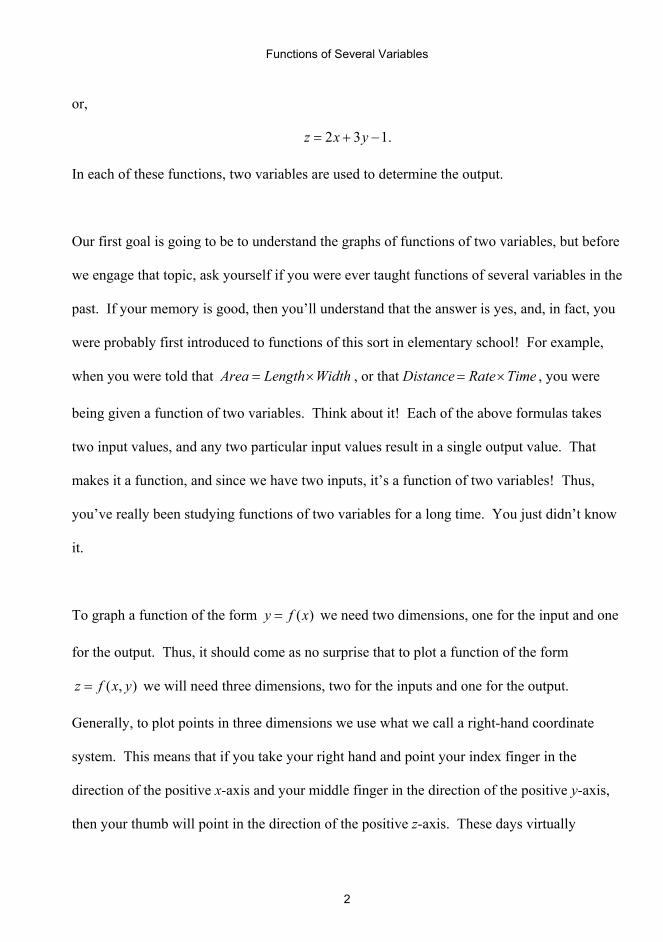
Generally, to plot points in three dimensions we use what we call a right-hand coordinate
system. This means that if you take your right hand and point your index finger in the
direction of the positive x-axis and your middle finger in the direction of the positive y-axis,
then your thumb will point in the direction of the positive z-axis. These days virtually
Functions of Several Variables
3
everyone uses a right-hand coordinate system, and a given point is located in space by
coordinates ( ), ,x y z
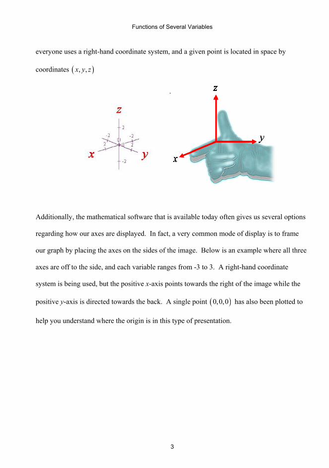
Additionally, the mathematical software that is available today often gives us several options
regarding how our axes are displayed. In fact, a very common mode of display is to frame
our graph by placing the axes on the sides of the image. Below is an example where all three
axes are off to the side, and each variable ranges from -3 to 3. A right-hand coordinate
system is being used, but the positive x-axis points towards the right of the image while the
positive y-axis is directed towards the back. A single point ( )0,0,0 has also been plotted to
help you understand where the origin is in this type of presentation.

Functions of Several Variables
4
Now let’s take a typical function of two variables and think about how we can analyze it. In
particular, let’s start with 2 2( , )z f x y x y= = + . What can we say about this function? Well,
it’s not hard to see that 2 2( , )z f x y x y= = + always has to be greater than or equal to zero.
In fact, the only time we will have 0z = is when 0x = and 0y = . This point, denoted by
( ) ( ), , 0,0,0 ,x y z = is also the lowest point on the graph. Furthermore, as we move away
from the origin in any direction, 2 2( , )z f x y x y= = + has to get larger. This already gives us
the image of some surface that has its lowest point at ( )0,0,0 and whose sides go up higher
and higher as we move away from that low point.
Functions of Several Variables
5
Now let’s think about some more sophisticated ways in which we might analyze the graph of
2 2( , )z f x y x y= = + . This next method is what I call “slicing and dicing.” For instance,
think of taking a cross-section of this surface by fixing a value of z such as 4z = . If we fix z
to 4, then our equation becomes 2 2 4x y+ = , and this is an equation for a circle of radius 2
with center at the origin. Similarly, if we fix z to any value whatsoever that is larger than
zero, we will likewise get a circular cross-section. Now try and visualize an object that has
its bottom point at ( )0,0,0 , rises upward as you move away from this point, and has circular
cross-sections when you slice through it by fixing the value of z.
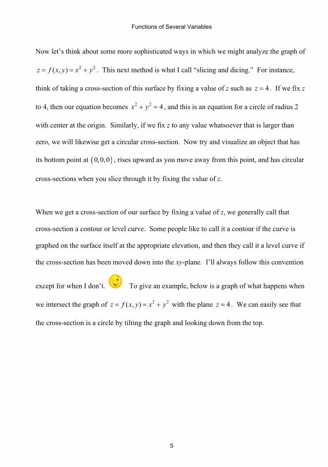
When we get a cross-section of our surface by fixing a value of z, we generally call that
cross-section a contour or level curve. Some people like to call it a contour if the curve is
graphed on the surface itself at the appropriate elevation, and then they call it a level curve if
the cross-section has been moved down into the xy-plane. I’ll always follow this convention
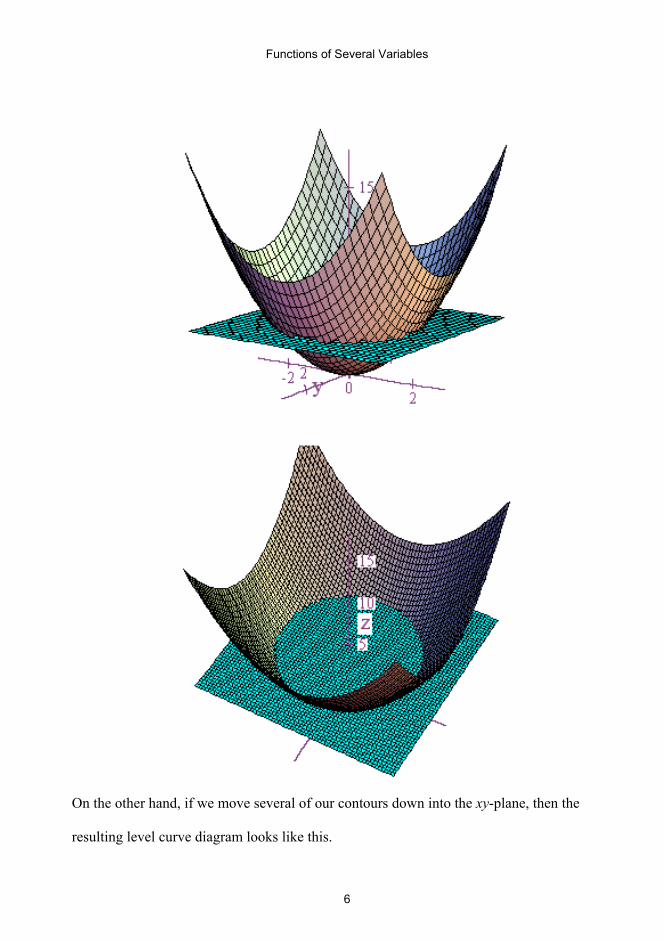
except for when I don’t. To give an example, below is a graph of what happens when
we intersect the graph of 2 2( , )z f x y x y= = + with the plane 4z = . We can easily see that
the cross-section is a circle by tilting the graph and looking down from the top.
Functions of Several Variables
6
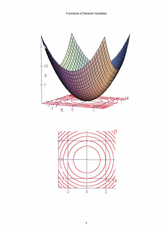
On the other hand, if we move several of our contours down into the xy-plane, then the
resulting level curve diagram looks like this.
Functions of Several Variables
7

Functions of Several Variables
8
This latter diagram is basically the same thing as a topographic map. A topographic map
such as the one below for a small hill gives us a 2-dimensional representation that helps us
more easily visualize the corresponding 3-dimensional surface. In a similar manner, level
curve diagrams also allow us to more easily capture in our minds the corresponding 3-
dimensional image.
We can do more slicing and dicing by fixing x and y to particular values. For example, if we
fix 2y = , then our cross-section is 2 4z x= + which is an equation for a parabola that opens
upward. Likewise, if we fix 2x = , then we get 24z y= + which is another equation for an
upward opening parabola. Thus, while cross-sections of 2 2( , )z f x y x y= = + created by
fixing z are circular, cross-sections created by fixing x or y will be parabolas. For this reason,
the graph of 2 2( , )z f x y x y= = + is usually called a paraboloid.
Up to this point, we’ve focused on how to analyze and visualize just parts of a graph, but
soon we will shift our focus to the entire graph itself. First, though, let’s do what we
normally do when we graph a function of one variable such as ( )y f x= . Let’s create a table

Functions of Several Variables
9
of values in order to give us some points to plot! Below is a table of values for
2 2( , )z f x y x y= = + where the x-values go from top to bottom on the left side while the y-
values are spaced left to right along the top. Both sets of values in this table range from -5 to
5. Additionally, in each individual cell you will find the z-value corresponding to the given x
and y. Then end result is as follows.
x\y -5 -4 -3 -2 -1 0 1 2 3 4 5-5 50 41 34 29 26 25 26 29 34 41 50-4 41 32 25 20 17 16 14 20 25 32 41-3 34 25 18 13 10 9 10 13 18 25 34-2 29 20 13 8 5 4 5 8 13 20 29-1 26 17 10 5 2 1 2 5 10 17 260 25 16 9 4 1 0 1 4 9 16 251 26 14 10 5 2 1 2 5 10 14 262 29 20 13 8 5 4 5 8 13 20 293 34 25 18 13 10 9 10 13 18 25 344 41 32 25 20 17 16 14 20 25 32 415 50 41 34 29 26 25 26 29 34 41 50
If we now plot the points in the table we created, here’s what we get.

Functions of Several Variables
10
The good news is, we’ve got a plot! The bad news is, it still doesn’t look like much. We just
lose too much perspective when we try to plot three dimensional points in two dimensions.
However, this is where slicing and dicing can help us. For example, let’s look at what
happens when we generate level curves by setting 2,5,z = or 8. The results are equations for
circles of radii 2, 5, and 8 , (i.e., 2 2 2 22, 5,x y x y+ = + = and 2 2 8x y+ = ). If we add
these circles at the appropriate elevation to our graph, then we get the following.

Functions of Several Variables
11
This certainly makes the graph a little easier to understand. However, let’s add to the
perspective even more by looking at the cross-sections that we get by setting x and y equal to
fixed values. First, we’ll set 1,0,y = − and 1. This gives us the equations 2 1z x= + , 2z x= ,
and 2 1z x= + . Add the graphs of these curves in the positions corresponding to 1,0,y = −
and 1, and we get the following.

Functions of Several Variables
12
Now we’re making some progress! Let’s refine our efforts even more by graphing the cross-
sections that we get by setting 1,0,x = − and 1, corresponding to 21z y= + , 2z y= , and
again 21 .z y= + Here’s what we get.

Functions of Several Variables
13
Now it’s really beginning to take shape! However, to tell the truth, we never really do things
quite this way. After all, if we have software that can do the kinds of graphs of cross-sections
that we’ve done above, then we can certainly use that software to simply draw the complete
graph to begin with, and when we do, we get something like this.

Functions of Several Variables
14
The point, though, is that we don’t always have such software available, and even if we do, it
still deepens our understanding if we are able to do some analysis of the function before
creating a computer generated image of the surface. For example, regarding the graph of
2 2( , )z f x y x y= = + , we were able to figure out the following.
1. The z-values are always greater than or equal to zero.
2. The lowest point is at (0,0,0).
3. The values of z increase as we move further away from the origin.
4. The cross-sections obtained by setting z equal to a constant are circles.
5. The cross-sections obtained by setting x or y equal to constant values are parabolas.
By doing this kind of analysis, we can get a pretty good idea beforehand of what the surface
graph will look like. And by the way, since many of the cross-sections of
Functions of Several Variables
15
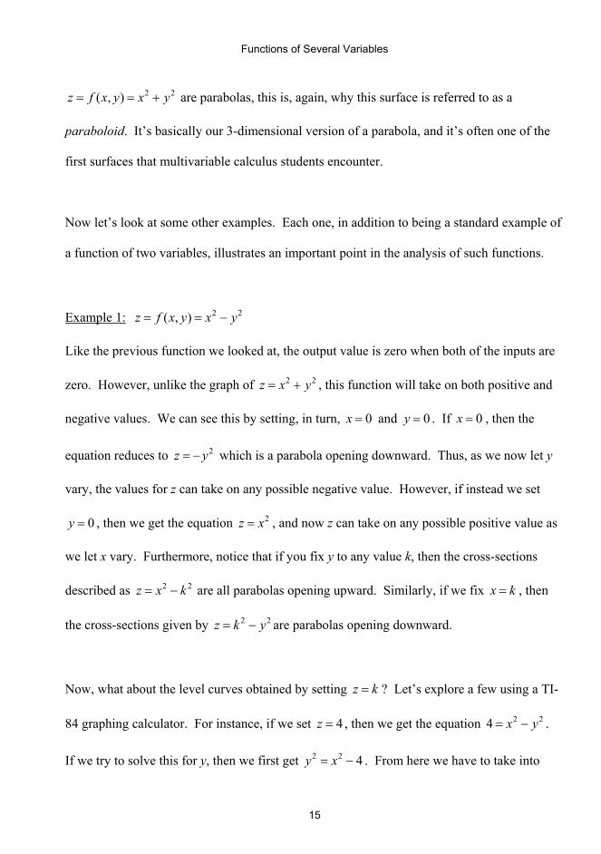
2 2( , )z f x y x y= = + are parabolas, this is, again, why this surface is referred to as a
paraboloid. It’s basically our 3-dimensional version of a parabola, and it’s often one of the
first surfaces that multivariable calculus students encounter.
Now let’s look at some other examples. Each one, in addition to being a standard example of
a function of two variables, illustrates an important point in the analysis of such functions.
Example 1: 2 2( , )z f x y x y= = −
Like the previous function we looked at, the output value is zero when both of the inputs are
zero. However, unlike the graph of 2 2z x y= + , this function will take on both positive and
negative values. We can see this by setting, in turn, 0x = and 0y = . If 0x = , then the
equation reduces to 2z y= − which is a parabola opening downward. Thus, as we now let y
vary, the values for z can take on any possible negative value. However, if instead we set
0y = , then we get the equation 2z x= , and now z can take on any possible positive value as
we let x vary. Furthermore, notice that if you fix y to any value k, then the cross-sections
described as 2 2z x k= − are all parabolas opening upward. Similarly, if we fix x k= , then
the cross-sections given by 2 2z k y= − are parabolas opening downward.
Now, what about the level curves obtained by setting z k= ? Let’s explore a few using a TI-
84 graphing calculator. For instance, if we set 4z = , then we get the equation 2 24 x y= − .
If we try to solve this for y, then we first get 2 2 4y x= − . From here we have to take into

Functions of Several Variables
16
account both positive and negative square roots to obtain 2 4y x= ± − . In order to graph
this on our calculator, we have to split it up into two functions, 21 4y x= − and
22 4y x= − − .
The shape of the graph is a hyperbola, and some of you may have recognized right off the bat
that 2 24 x y= − is an equation for a hyperbola that crosses the x-axis at -2 and 2. Similarly, if
we set 4z = − , then we get the equation 2 24 x y− = − which is another hyperbola. However,
this time we have y-intercepts of -2 and 2, and no x-intercepts.
Almost all values of z give us hyperbolas. The only exception is if we set 0z = . In this case,
we get 2 2 2 20 x y y x y x= − ⇒ = ⇒ = ± . When we graph the last equation, we get two
straight lines that intersect at the origin.

Functions of Several Variables
17
Now let’s look at a computer-generated graph along with the level curves.
Functions of Several Variables
18
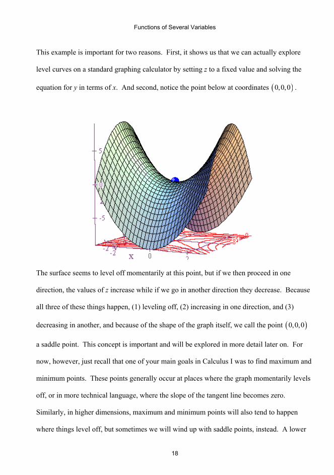
This example is important for two reasons. First, it shows us that we can actually explore
level curves on a standard graphing calculator by setting z to a fixed value and solving the
equation for y in terms of x. And second, notice the point below at coordinates ( )0,0,0 .
The surface seems to level off momentarily at this point, but if we then proceed in one
direction, the values of z increase while if we go in another direction they decrease. Because
all three of these things happen, (1) leveling off, (2) increasing in one direction, and (3)
decreasing in another, and because of the shape of the graph itself, we call the point ( )0,0,0
a saddle point. This concept is important and will be explored in more detail later on. For
now, however, just recall that one of your main goals in Calculus I was to find maximum and
minimum points. These points generally occur at places where the graph momentarily levels
off, or in more technical language, where the slope of the tangent line becomes zero.
Similarly, in higher dimensions, maximum and minimum points will also tend to happen
where things level off, but sometimes we will wind up with saddle points, instead. A lower

Functions of Several Variables
19
dimensional version of a saddle point could be something like the point ( )0,0 on the graph of
3y x= . Here, once again, we might say there is leveling off, but no cigar. No maximum or
minimum.
Example 2: 2 3z x y= + +
Let’s think for a moment about what’s going to happen with this function. If we fix a value
of y, then we get z as a linear function of x. For example, set 0,1,2,&3y = , in turn, and we
get back the linear equations 3z x= + , 5z x= + , 7z x= + , and 9z x= + . All of these
equations represent lines of slope 1, and if we graph them in the appropriate locations in 3-
dimensional space, then we start to see that the graph of 2 3z x y= + + is a plane.
Functions of Several Variables
20
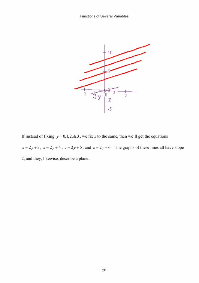
If instead of fixing 0,1,2,&3y = , we fix x to the same, then we’ll get the equations
2 3z y= + , 2 4z y= + , 2 5z y= + , and 2 6z y= + . The graphs of these lines all have slope
2, and they, likewise, describe a plane.

Functions of Several Variables
21
A few things should be clear at this point. Namely,
1. Cross-sections of a plane obtained by fixing a value of y will be straight lines, and
these lines will all have the same slope.
2. Cross-sections of a plane obtained by fixing a value of x will be straight lines, and
these lines will all have the same slope.
3. The slope of the linear cross-sections obtained by fixing a value of y represents the
rate at which z changes with respect to x as we move in the direction of the positive
x-axis.
4. The slope of the linear cross-sections obtained by fixing a value of x represents the
rate at which z changes with respect to y as we move in the direction of the positive
y-axis.
Functions of Several Variables
22
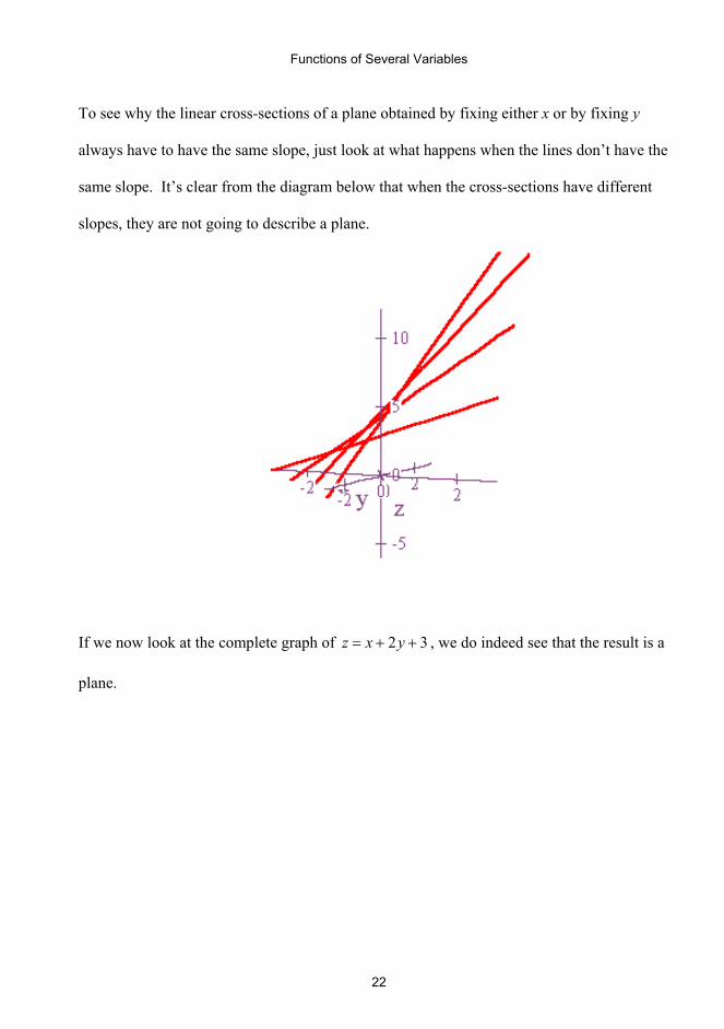
To see why the linear cross-sections of a plane obtained by fixing either x or by fixing y
always have to have the same slope, just look at what happens when the lines don’t have the
same slope. It’s clear from the diagram below that when the cross-sections have different
slopes, they are not going to describe a plane.
If we now look at the complete graph of 2 3z x y= + + , we do indeed see that the result is a
plane.

Functions of Several Variables
23
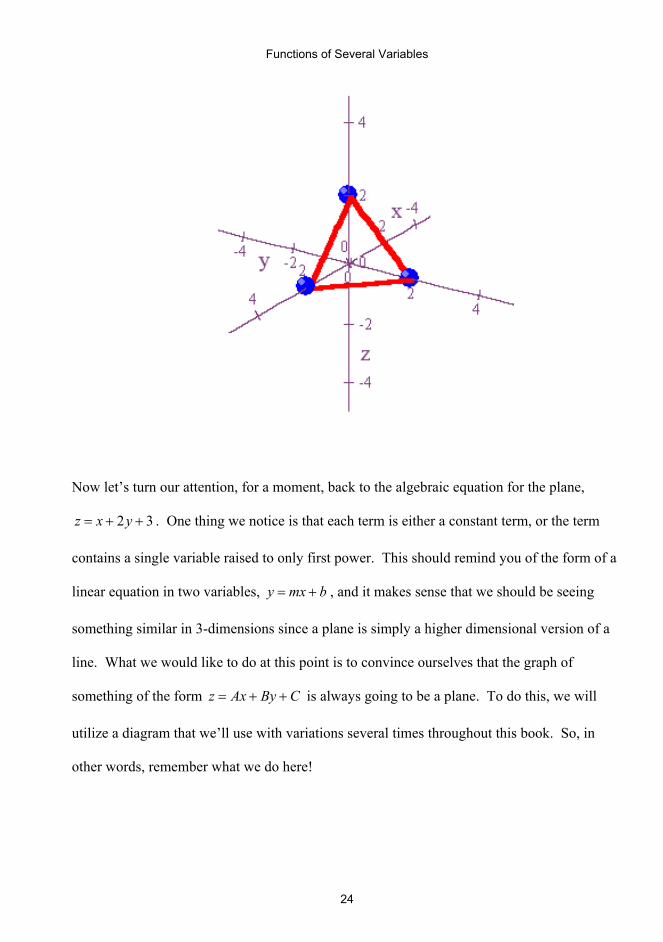
If we are trying to graph a plane such as 2 3z x y= + + by hand, then the easiest way to do it
is often by plotting the x-, y-, and z-intercepts. As long as these three points are distinct, this
method works well. Below is what we get for the plane 2x y z+ + = , and simply connecting
these three dots is enough to give us an idea of what the final plane looks like.
Functions of Several Variables
24
Now let’s turn our attention, for a moment, back to the algebraic equation for the plane,
2 3z x y= + + . One thing we notice is that each term is either a constant term, or the term
contains a single variable raised to only first power. This should remind you of the form of a
linear equation in two variables, y mx b= + , and it makes sense that we should be seeing
something similar in 3-dimensions since a plane is simply a higher dimensional version of a
line. What we would like to do at this point is to convince ourselves that the graph of
something of the form z Ax By C= + + is always going to be a plane. To do this, we will
utilize a diagram that we’ll use with variations several times throughout this book. So, in
other words, remember what we do here!

Functions of Several Variables
25
In this diagram, we show a plane that contains the point ( ), ,a b c and the point ( ), ,x y z . As
we move from the first point to the second, there is a change in x, a change in y, and a change
in z. We denote these, respectively, by x x aΔ = − , y y bΔ = − , and z z cΔ = − . Notice also
that the slope of a cross-section in the direction of the positive x-axis is 1zx
ΔΔ
, the slope of a
cross-section in the direction of the positive y-axis is 2zy
ΔΔ
, and 1 2z z zΔ = Δ + Δ . If we call the
slope in the direction of the positive x-axis xm and the slope in the direction of the positive y-
axis ym , then 1x
zmx
Δ=Δ
and 2y
zmy
Δ=Δ
imply that 1 xz m xΔ = Δ and 2 yz m yΔ = Δ . From this
it follows that 1 2 x yz z z m x m yΔ = Δ + Δ = Δ + Δ . If we now replace the changes in x, y, and z by
the expressions we have above, then we get ( ) ( )x yz c m x a m y b− = − + − which could be
written in a more general form as z Ax By C= + + . In this form, A is the slope of the linear
cross-section as one moves in the direction of the positive x-axis, and B is the slope in the
direction of the positive y-axis. Notice, too, that 0Az Bx Cy D+ + + = is just a variation of
xΔ1zΔ
2zΔ
( , , )a b c
( , , )x y z
yΔ 1 2z z zΔ = Δ + Δ}xΔ
1zΔ
2zΔ
( , , )a b c
( , , )x y z
yΔ 1 2z z zΔ = Δ + Δ}
Functions of Several Variables
26
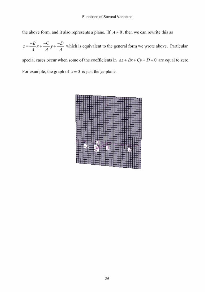
the above form, and it also represents a plane. If 0A ≠ , then we can rewrite this as
B C Dz x yA A A− − −
= + + which is equivalent to the general form we wrote above. Particular
special cases occur when some of the coefficients in 0Az Bx Cy D+ + + = are equal to zero.
For example, the graph of 0x = is just the yz-plane.

Functions of Several Variables
27
The graph of 0y = is the xz-plane.
And the graph of 0z = is the xy-plane.

Functions of Several Variables
28
If we return for a moment to the function we started this example with, 2 3z x y= + + , below
is the graph of this plane along with its level curves.

Functions of Several Variables
29
Notice that not only are the level curves straight lines, they also appear to be evenly spaced.
Level curves are usually constructed so that the change in z is always the same as we go from
one curve to the next, and when the curves are also evenly spaced as we move in either the
positive x or y direction, then this shows that the values for z are changing at a constant rate
with respect to both x and y. This is exactly what we expect to happen since if we fix either
the x or the y value, then the cross-section is a straight line, and straight lines have a constant
rate of change. In the next example, though, we’ll see what happens when the level curves
are straight lines, but the rate of change of z with respect to one of the other variables is not
constant.
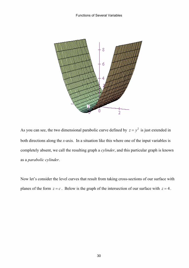
Example 3: 2z y=
In this function there is no x variable. What this means is simply that the value of x doesn’t
matter. In other words, the value of z is completely determined by y. As a result, if we take
cross-sections by fixing values for x, then we’ll always get the same parabolic curve as our
cross-section. Below is the graph of 2z y= .
Functions of Several Variables
30
As you can see, the two dimensional parabolic curve defined by 2z y= is just extended in
both directions along the x-axis. In a situation like this where one of the input variables is
completely absent, we call the resulting graph a cylinder, and this particular graph is known
as a parabolic cylinder.
Now let’s consider the level curves that result from taking cross-sections of our surface with
planes of the form z c= . Below is the graph of the intersection of our surface with 4z = .

Functions of Several Variables
31
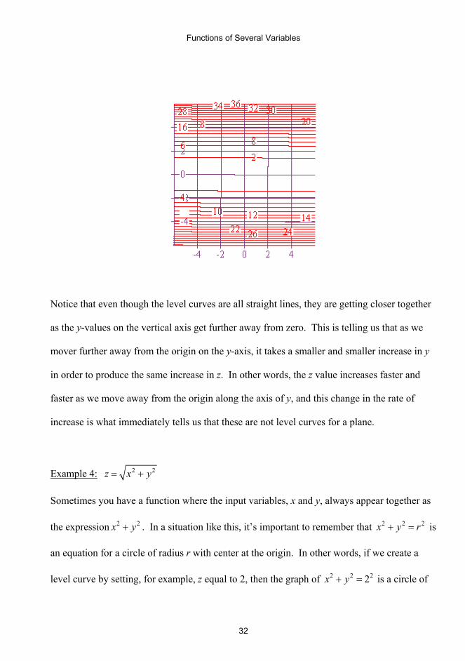
We can see quite easily that the cross-section is a pair of lines. If we now look at a more
complete graph of the level curves, we get something like the diagrams below.
Functions of Several Variables
32
Notice that even though the level curves are all straight lines, they are getting closer together
as the y-values on the vertical axis get further away from zero. This is telling us that as we
mover further away from the origin on the y-axis, it takes a smaller and smaller increase in y
in order to produce the same increase in z. In other words, the z value increases faster and
faster as we move away from the origin along the axis of y, and this change in the rate of
increase is what immediately tells us that these are not level curves for a plane.
Example 4: 2 2z x y= +
Sometimes you have a function where the input variables, x and y, always appear together as
the expression 2 2x y+ . In a situation like this, it’s important to remember that 2 2 2x y r+ = is
an equation for a circle of radius r with center at the origin. In other words, if we create a
level curve by setting, for example, z equal to 2, then the graph of 2 2 22x y+ = is a circle of
Functions of Several Variables
33
radius 2 with center at the origin. More generally, every level curve of 2 2z x y= + is a
circle with radius z.
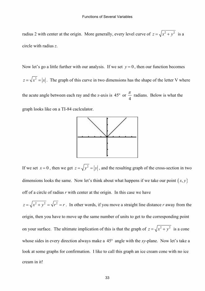
Now let’s go a little further with our analysis. If we set 0y = , then our function becomes
2z x x= = . The graph of this curve in two dimensions has the shape of the letter V where
the acute angle between each ray and the x-axis is 45° or 4π radians. Below is what the
graph looks like on a TI-84 caclculator.
If we set 0x = , then we get 2z y y= = , and the resulting graph of the cross-section in two
dimensions looks the same. Now let’s think about what happens if we take our point ( ),x y
off of a circle of radius r with center at the origin. In this case we have
2 2 2z x y r r= + = = . In other words, if you move a straight line distance r away from the
origin, then you have to move up the same number of units to get to the corresponding point
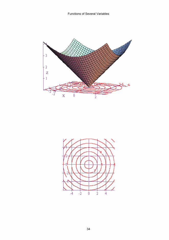
on your surface. The ultimate implication of this is that the graph of 2 2z x y= + is a cone
whose sides in every direction always make a 45° angle with the xy-plane. Now let’s take a
look at some graphs for confirmation. I like to call this graph an ice cream cone with no ice
cream in it!
Functions of Several Variables
34

Functions of Several Variables
35
Example 5: 2 21z
x y−
=+
Like the previous function, this one also has the input variables bundled together in the
expression 2 2x y+ . This means that the level curves obtained by fixing values of z will also
be circles. Additionally, we can also make the following observations.
1. The values for z are always negative.
2. The function is undefined at the origin.
3. The z values get larger in magnitude in the negative direction as both x and y get
closer to 0.
4. The z values get closer to 0 as either x or y gets further from the origin.
The end result is a graph that looks like the proverbial black hole as it is sometimes depicted
graphically in movies.

Functions of Several Variables
36
Example 6: 2 2cos( )z x y= +
Once again we see the expression 2 2x y+ , and we know that the level curves will be circles,
or in this case, a horizontal plane can intersect the surface in many concentric circles since the
cosine function is periodic with period 2π . Let’s now think for a moment, though, about
what’s going to happen as both x and y move away from the origin. When the input values
get far away from the origin, we usually refer to what happens as the end or long run behavior
of the graph. While you might think that such things are complicated, in practice only a few
things generally happen. With most functions the long run behavior is generally either that z
gets large in the positive direction, z gets large in the negative direction, z becomes
asymptotic to some fixed value, or z oscillates or jumps around between values. For our

Functions of Several Variables
37
function above, it’s going to be the latter that happens. For example, since z is defined as the
cosine of something, we know immediately that the output is going to oscillate between -1
and 1, and , as mentioned, a given output value will often correspond to several circles in the
xy-plane. For example, the circles 2 2 2x y π+ = , 2 2 4x y π+ = , and 2 2 6x y π+ = will all be
associated with the output value 1z = . Let’s now look at the surface and its level curves. As
deduced above, the level curve diagram consists of concentric circles.

Functions of Several Variables
38
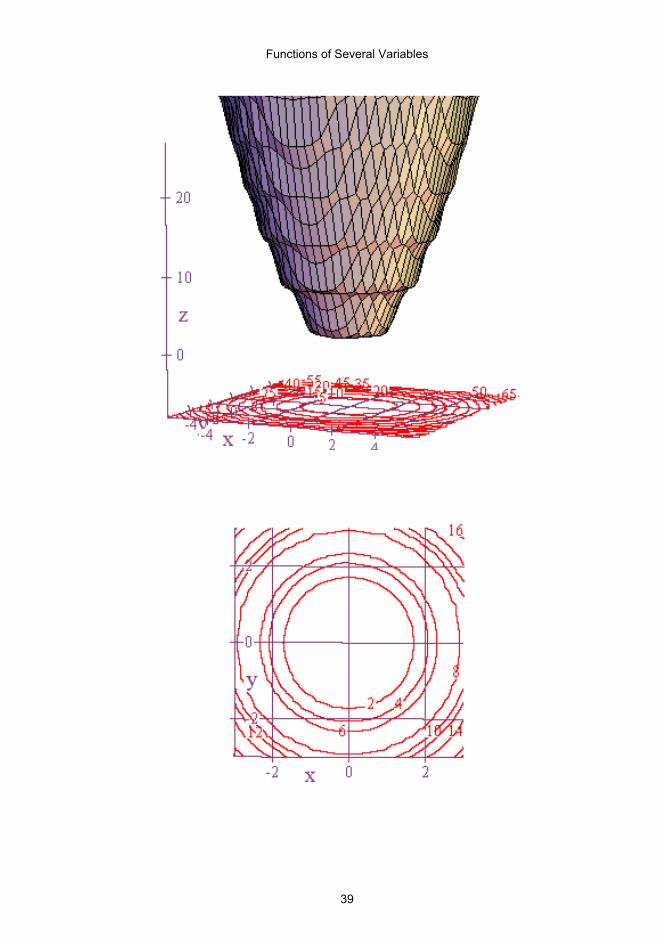
Now let’s think about what happens if we change our function to
2 2 2 2cos( ) ( )z x y x y= + + + . This time, the z values should increase as x and y move further
from the origin, but the level curves should still be circles since we never find 2x without a
2y being added to it. Here is the graph. As we move away from the origin, the z values
increase, but our cosine term, nevertheless, still creates some oscillation in the output.
Functions of Several Variables
39
Functions of Several Variables
40
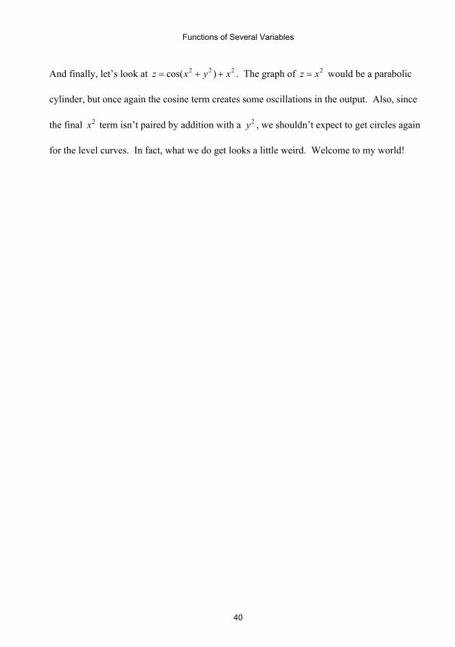
And finally, let’s look at 2 2 2cos( )z x y x= + + . The graph of 2z x= would be a parabolic
cylinder, but once again the cosine term creates some oscillations in the output. Also, since
the final 2x term isn’t paired by addition with a 2y , we shouldn’t expect to get circles again
for the level curves. In fact, what we do get looks a little weird. Welcome to my world!
Functions of Several Variables
41
Functions of Several Variables
42
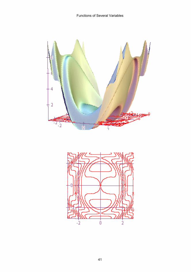
Now let’s have a little fun! Below are four level curve diagrams, but only one of them
corresponds to the function 2 1z x y= − + + . Can you tell which one it is?
a. b.
c. d.
Since 2 1z x y= − + + is an equation for a plane, the level curves have to be straight lines
and so the answer can’t be a. Also, since z has to have a constant rate of change with respect
to both the positive x direction and the positive y direction, the answer can’t be b. In b, the
level curves are getting closer together as we move further away from zero along the x-axis,
and this means that the value of z is changing at an ever faster rate. Having eliminated both a
and b, that leaves only c and d, and now things are trickier because both of these level curve
diagrams do look like they represent planes. However, what we need to remember here is
Functions of Several Variables
43
that in the equation 2 1z x y= − + + , the coefficient of x tells us the rate at which z is
changing with respect to movement in the direction of the positive x-axis, and the coefficient
of y tells us the rate at which z is changing with respect to movement in the direction of the
positive y-axis. What we see from these coefficients is that z should decrease as x increases,
and z should increase as y increases. The only diagram for which this happens is d, and so d
is the correct level curve diagram for 2 1z x y= − + + .
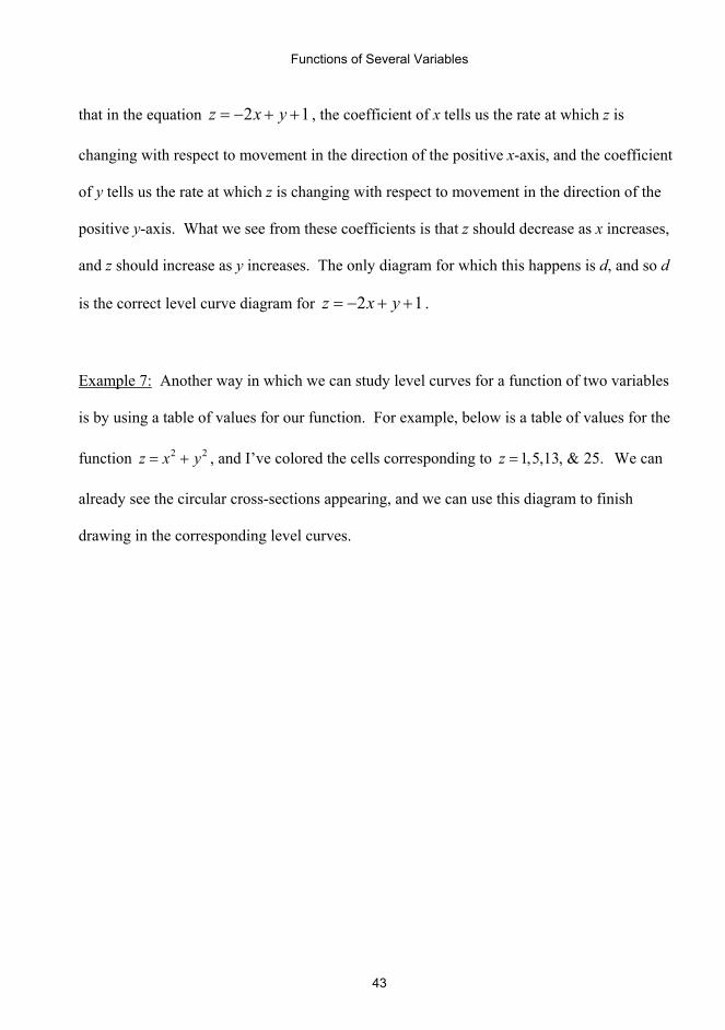
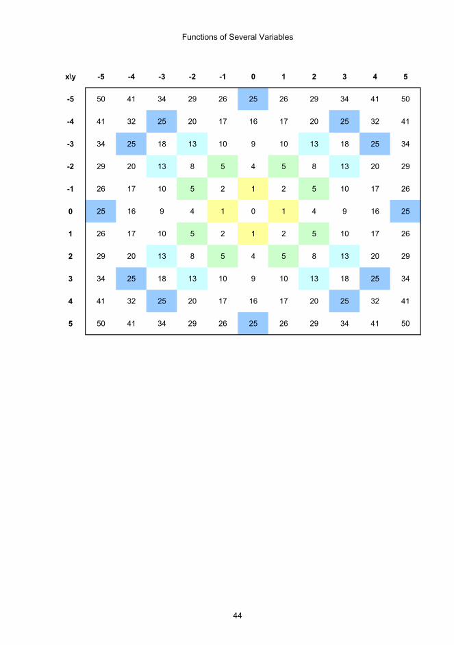
Example 7: Another way in which we can study level curves for a function of two variables
is by using a table of values for our function. For example, below is a table of values for the
function 2 2z x y= + , and I’ve colored the cells corresponding to 1,5,13, & 25.z = We can
already see the circular cross-sections appearing, and we can use this diagram to finish
drawing in the corresponding level curves.
Functions of Several Variables
44
x\y -5 -4 -3 -2 -1 0 1 2 3 4 5
-5 50 41 34 29 26 25 26 29 34 41 50
-4 41 32 25 20 17 16 17 20 25 32 41
-3 34 25 18 13 10 9 10 13 18 25 34
-2 29 20 13 8 5 4 5 8 13 20 29
-1 26 17 10 5 2 1 2 5 10 17 26
0 25 16 9 4 1 0 1 4 9 16 25
1 26 17 10 5 2 1 2 5 10 17 26
2 29 20 13 8 5 4 5 8 13 20 29
3 34 25 18 13 10 9 10 13 18 25 34
4 41 32 25 20 17 16 17 20 25 32 41
5 50 41 34 29 26 25 26 29 34 41 50

Functions of Several Variables
45
By following the same procedure for the function 2 2z x y= − , we can use this function’s
table of values to help us replicate the lines and hyperbolas found in its level curve diagram.

Functions of Several Variables
46
x\y -5 -4 -3 -2 -1 0 1 2 3 4 5
-5 0 9 16 21 24 25 24 21 16 9 0
-4 -9 0 7 12 15 16 15 12 7 0 -9
-3 -16 -7 0 5 8 9 8 5 0 -7 -16
-2 -21 -12 -5 0 3 4 3 0 -5 -12 -21
-1 -24 -15 -8 -3 0 1 0 -3 -8 -15 -24
0 -25 -16 -9 -4 -1 0 -1 -4 -9 -16 -25
1 -24 -15 -8 -3 0 1 0 -3 -8 -15 -24
2 -21 -12 -5 0 3 4 3 0 -5 -12 -21
3 -16 -7 0 5 8 9 8 5 0 -7 -16
4 -9 0 7 12 15 16 15 12 7 0 -9
5 0 9 16 21 24 25 24 21 16 9 0
And here is what the corresponding level curve diagram should look like.
Functions of Several Variables
47
Up to this point, pretty much all of the functions we’ve looked at have been abstract,
mathematical functions of two variables, and for a while longer we will continue to look at
things from a pure mathematical perspective. Nonetheless, keep in mind that everything that
we are doing can also serve as a mathematical model for real world situations. For example,
in a real world context, our input variables might represent levels of production in a factory
for different products, and the output variable could be the corresponding profit generated.
Or the input variables could represent a person’s height and weight, and the output could be
the probability of a person having approximately that height and weight. We’ll see a variety
of real world problems later on, and for those problems the units attached to the variables will
provide a practical context for our answers. For now, however, we will continue studying
things at a purely abstract level.
For the final set of examples, I just want to present a catalog of some of my favorite graphs of
functions of two variables. Each is a basic example in its own way, and several of them
we’ve seen before. Nevertheless, study them well, contemplate why the graphs look the way
they do, and enjoy!

Functions of Several Variables
48
1. 2 2z x y= +
2. 2 2z x y= −
Functions of Several Variables
49
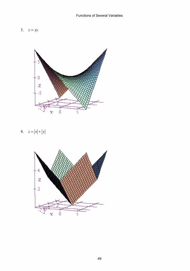
3. z xy=
4. z x y= +

Functions of Several Variables
50
5. ( )2 2lnz x y= +
6. 2 1z x y= − + +

Functions of Several Variables
51
7. 2z x=
8. 2 2z x y= +
Functions of Several Variables
52
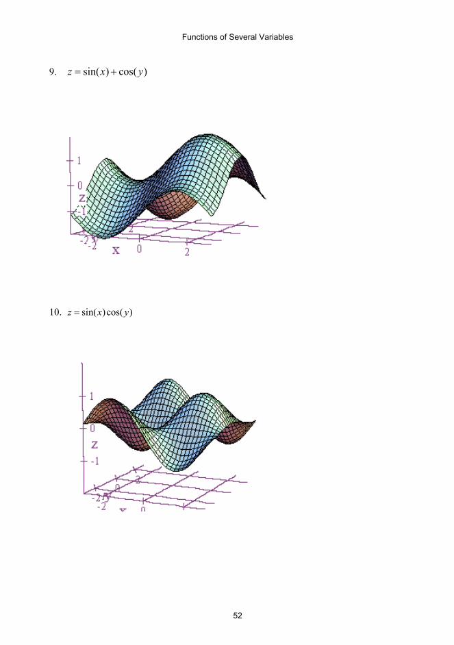
9. sin( ) cos( )z x y= +
10. sin( )cos( )z x y=

Functions of Several Variables
53
11. 2 2( )x yz e− +=
12. 3 2z x xy= −

Functions of Several Variables
54
13. sin( )sin( )x yzxy
=
14. 2 2
2 2
sin x yz
x y
+=
+

Functions of Several Variables
55
15. 2z y x= +
16. z x y= +
Functions of Several Variables
56
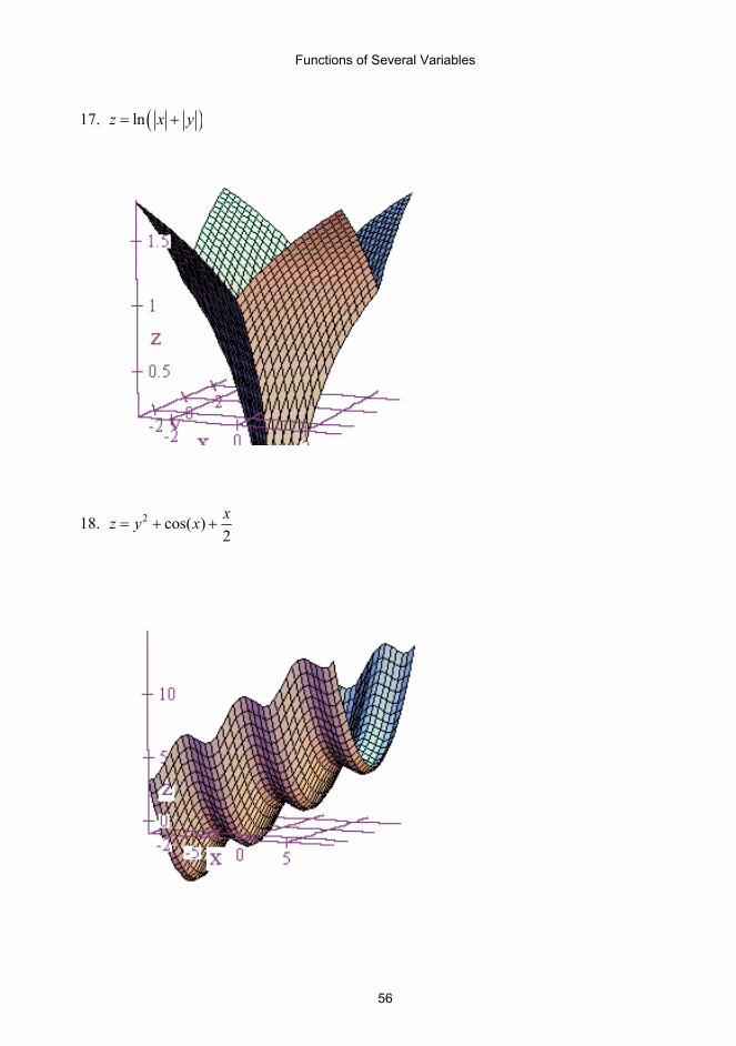
17. ( )lnz x y= +
18. 2 cos( )2xz y x= + +

Functions of Several Variables
57
19. 2 2
2 2( )xy x yzx y
−=
+