chapter 1 – introducing input-output analysis at the regional
TRANSCRIPT

The Regional Economics Applications Laboratory (REAL) is a unit of the University of Illinois focusing on the development and use of analytical models for urban and region economic development. The purpose of the Discussion Papers is to circulate intermediate and final results of this research among readers within and outside REAL. The opinions and conclusions expressed in the papers are those of the authors and do not necessarily represent those of the University of Illinois. All requests and comments should be directed to Geoffrey J. D. Hewings, Director, Regional Economics Applications Laboratory, 607 South Matthews, Urbana, IL, 61801-3671, phone (217) 333-4740, FAX (217) 244-9339. Web page: www.real.illinois.edu.
INTRODUCING INPUT-OUTPUT ANALYSIS AT THE REGIONAL LEVEL: BASIC NOTIONS AND SPECIFIC ISSUES.
Ana Lúcia Marto Sargento*
REAL 09-T-4 July, 2009
* School of Technology and Management, Polytechnic Institute of Leiria, Portugal [email protected]

Notation Variables:
ix - output of product i;
ijz - Amount of product i used as an intermediate input in the production of industry j;
jw - value added in industry j;
jm - total imports of product j;
iy - Final demand for product i (it includes: final consumption, gross capital formation and
exports); rix - output of product i in region r;
rie - regional production of product i;
rijz - total amount of product i (regionally produced and imported) used as an intermediate input
in the production of industry j, in region r; rrijz - amount of regionally produced product i used as an intermediate input in the production of
industry j, in region r; r
if - region’s final demand for product i produced in region r (including regional requirements
as well as exports for any other regions, national or foreign); riy - regional final demand for product i;
rsijz - amount of product i coming from region r that is used as an intermediate input by industry j
in region s; srix - amount of product i shipped by region s to region r, without specifying the type of buyer in
the region of destination. riR - total amount of product i available in region r, except for foreign imports;
rsif - amount of product i produced in region r and shipped to region s.
sijz • - total amount of product i (produced in region s and in the other regions of the same
country) used as an input by industry j in region s;
* School of Technology and Management, Polytechnic Institute of Leiria, Portugal [email protected]
ijv - domestic production of product j by industry i (elements of the Make matrix – rectangular
model);

Input-Output Analysis at the Regional Level 3
jiu - the amount of product j used as an input in the production of industry i’s output (elements
of the Use matrix – rectangular model);
jp - total supply of product j (rectangular model);
ig - domestic production of industry i (sum of the rows of the Make matrix);
rjAO - available output in region r to satisfy domestic demand (demand directed to region r and
also to the remaining regions of the country). rjD - total requirements of i in region r.
rocrjd - exports from region r to the rest of the country.
rrocjm - imports from the rest of the country to region r.
rrocj
rocrj
rj deNEX −= - net exports of product j by region r.
i - column vector appropriately dimensioned, composed by 1’s.
^ - diagonal matrix.
Superscript row – coming from (or going to) the rest of the world.
Superscript roc – coming from (or going to) the rest of the country.
Coefficients:
ija - technical coefficient (at national level);
ijb - generic element of the Leontief inverse matrix;
jb• - output multiplier ( ); ∑=•i
ijj bb
rija - regional technical coefficient; r
j
rijr
ij xz
a = ;
rrija - intra-regional input coefficient; r
j
rrijrr
ij ez
a = ;
rsija - interregional trade coefficient, representing the amount of input i from region r necessary
per monetary unit of product j produced in region s; sj
rsijrs
ij ez
a = ;

Input-Output Analysis at the Regional Level 4
srit - trade coefficient, representing the proportion of product i available in region r that comes
from region s; ri
srisr
i Rx
t = ;
sj
sijs
ij ez
a•
• = - technical coefficient for region s: it represents the amount of product i necessary to
produce one unit of industry j’s output in region s, considering the inputs provided by all the
regions in the system.
i
jiji g
uq = - Technical coefficient in the rectangular model (amount of product j used as input in
the production of one unit of industry i’s output);
j
ijij p
vs = - industry i’s market share in product j’s total supply.
Matrices and vectors:
I - identity matrix;
x - output vector;
y - final use vector;
A - technical coefficients matrix;
B - Leontief’s inverse; rA - regional technical coefficients matrix ;
ry - regional final demand vector; rx - regional output vector; re - vector of output produced in region r; rrZ - matrix if intra-regional intermediate use flows; rrA - intra-regional input coefficients matrix;
rf - vector of regional final demand for products produced in region r. rsA - interregional trade coefficient matrix;
rsT - matrix of trade coefficients in the main diagonal; rsit
Q - technical coefficient matrix (rectangular model);

Input-Output Analysis at the Regional Level 5
g - vector of industries’ internal production (rectangular model);
U - intermediate consumption matrix (rectangular model);
V - Make matrix (rectangular model);
S - matrix of market shares ; (industry-based technology assumption on the rectangular
model);
ijs
p - Vector of products’ total supply (rectangular model);

Input-Output Analysis at the Regional Level 6
Abstract: This paper reviews the literature on regional input-output model estimation with particular attention to the development of interregional input-output models under conditions of limited information. The review covers simple nonsurvey estimation to more sophisticated approaches drawing on gravity and spatial interaction concepts, bi-proportional matrix adjustments and information theory applications. The review considers issues in traditional interindustry and commodity-industry accounting frameworks.
1. Introduction The main objective of the well known input-output model, developed by Leontief in the late
1930s, is to study the interdependence among the different sectors in any economy (Miller and
Blair, 1985). This tool holds upon a very simple, yet essential notion, according to which the
output is obtained through the consumption of production factors (inputs) which can be, in their
turn, the output of other industries. Hence, one of the principal tasks of input-output analysis is
to identify the indirect demands concerning the intermediate consumptions necessary to generate
the outputs.
The origins of the basic notion behind the input-output model go back to the 18th century, when
Quesnay published the “Tableau Economique.” His objective was to describe the economic
transactions established between three social classes: landowners, farmers and rural workers
(productive class) and the sterile class, composed by artisans and merchants (this classification
reflects the physiocrats’ philosophy, according to which agriculture was the only wealth
generating sector).
Over more than one century, this idea of economic interdependence had a new and important
contribution, with the work developed by Walras.1 This economist introduced the general
equilibrium model, aiming to determine prices and quantities of all economic markets. In this
model Walras used a set of production coefficients very similar to the ones defined a posteriori
in the Leontief’s input-output model: they compared the amount of production factors used in
production with the total output obtained (Miller and Blair, 1985).
The perception and depiction of the interactions among the different economic activities (besides
the spatial dimension which is being considered) allows, on the one hand, the access to a very
detailed statistical tool about the economy we are focusing on: the input-output table. An input-
output table records the “flows of products from each industrial sector considered as a producer
to each of the sectors considered as consumers” (Miller and Blair, 1985, p. 2). This table gives
1 Walras, L. 1874. “Elements of pure economics”. Translated by W. Jaffé. Homewood, Illinois: Richard Irwin, Inc., 1954. Referred in Miller and Blair (1985).

Input-Output Analysis at the Regional Level 7
us a quite complete picture of the economy at some specific point in time, providing estimates
for an important set of macroeconomic aggregates (production, demand components, value
added and trade flows) and disaggregating these among the different industries and products.
Besides, the input-output table is a suitable instrument to perform structural analysis of the
correspondent economy, depicting the interdependence between its different sectors and between
the economy and the rest of the world (ISEG/CIRU, 2004). On the other hand, the input-output
table provides an important database to the construction of input-output models which may be
used, for example, to evaluate the economic impact caused by exogenous changes in final
demand (Miller, 1998).
The original applications of the input-output model were made at a nation-wide level.2
However, the interest in extending the application of the same framework to spatial units
different from the country (usually, sub-national regions) led to some modifications in the
national model, originating a set of regional input-output models. According to Miller and Blair
(1985), there are two specific characteristics referring to the regional dimension which make
evident and necessary the distinction between national and regional input-output models. First,
the productive structure of each region is specific, probably being very different from the
national one; second, the smaller the focusing economy, the more it depends on the exterior
world (this including the other regions of the same country and other countries), making exports
and imports to become more important in determining the region’s demand and supply.
Since the 1950’s, different regional input-output models were developed, being distinguished
through the following criteria: (1) the number of regions taken into account; (2) the recognition
(or not) of interregional linkages; (3) the degree of detail implicit in interregional trade flows
(which is related to the degree of detail demanded for the input-output data) and (4) the kind of
hypotheses assumed to estimate trade coefficients. The first criterion is used to distinguish the
single-region model from the several types of models designed to systems with more than one
region. The single-region model seeks to capture intra-regional effects alone. So, its crucial
limitation consists of the fact that it ignores the effects caused by the linkages between this
region and the others. In reality, when one region increases its production, as a reaction to some
exogenous change in its final demand for example, some of the inputs needed to answer the
2 An example of this is the pioneering application of Leontief to the United States that became public through the book “The Structure of the American Economy, 1919-1929”, published for the first time in 1941.

Input-Output Analysis at the Regional Level 8
production augment will come from the remaining regions, originating an increase of production
in these regions – these are the spillover effects. The remaining regions, in turn, may need to
import inputs from other regions (probably including the first region) to use in their own
production. These involve the concept of interregional feedback effects: those which are caused
by the first region itself, through the interactions it performs with the remaining regions (Miller,
1998). The seminal applications of input-output analysis to systems with more that one region,
capturing the effects caused by the interconnections between the different regions (which
corresponds to the second criterion previously referred), had the fundamental contributions of
Walter Isard (Glasmeier, 2004). These contributions originated the interregional model also
known as Isard’s model. Practical difficulties in implementing the interregional model, mainly
due to its high requirements in terms of interregional trade data, motivated the emergence of
multi-regional models (of which the Chenery-Moses model is the most popular). As we shall see
latter on in this paper, the different many-region models are distinguishable through the third and
fourth criteria mentioned above.
This brief introduction to regional input-output models makes clear that their implementation
requires the access to some data on interregional trade flows (more or less detailed, depending on
the specific type of regional input-output model). How relevant are actually interregional trade
flows to regional economies? Some regional studies have proved that trade flows established
between one region and the remaining regions tend to be more significant than trade flows
established between the same region and foreign countries (Munroe et al., 2007). Moreover,
interregional trade is indeed growing faster than intra-regional and international trade (Jackson et
al., 2004). One of the reasons for the rapid growth of interregional trade is the fact that it is
currently replacing much of the intra-regional transactions, in a process called “hollowing-out”:
it implies that the density of relations within the regional economy tends to diminish, in favor of
interregional linkages (Polenske and Hewings, 2004). Given its relative importance in the
region’s external trade, the knowledge of the volume and nature of interregional trade flows
constitutes a critical issue for regional analysis. For example, a deficit in the region’s trade
balance means that the region relies on income transfer and/or granting of savings from other
regions, within the country or from the rest of the world (Ramos and Sargento, 2003). In a more
detailed perspective, knowledge about regional external trade, segmented by commodities,
allows us to characterize productive specialization, foresee eventual productive weaknesses as

Input-Output Analysis at the Regional Level 9
well as determine the region’s dependency on the exterior (or in some cases the exterior’s
dependency on the region) regarding to the supply of different commodities. In spite of its
recognized importance, interregional trade flows established between regions of the same
country constitute precisely the hardest data to find among the set of data necessary to implement
the input-output model.
The previous paragraph leads us to the first of the fundamental issues underlying the present
work, which also constitutes one of the main challenges of regional input-output researchers:
obtaining the regional data necessary to implement input-output models, with special concern in
interregional trade. The existing regional data, provided by the official organisms of statistics, is
usually “less than perfect”, meaning that it is more or less distant from the ideal set of data
required by each type of regional input-output model. Facing this problem, the researcher may
follow two alternatives (or do both): adapt the model to the existing data and / or estimate (or
directly collect) the inexistent data. Even when some adaptation is made, through the use of
some assumptions, a minimum amount of data on interregional trade (besides other input-output
table components) is always necessary, so that the model succeeds in capturing spillover and
feedback effects caused by the interregional linkages. As a result, some techniques must be
adopted to assess those data. These techniques can be classified according to the degree of
incorporation of direct regional information. Most of the researchers use hybrid methods,
combining some survey information with non-survey techniques, in which specific regional
indicators are applied to convert national values into regional ones. There is a general consensus
that the more direct information is incorporated in the table, the more accurately it tends to
reflect regional reality. However, the introduction of direct information implies higher costs,
which forces the researcher to make this in a selective way (more or less restrictively, depending
on the resources available to conduct regional surveys). Besides, even if the research team does
not face any restrictions in terms of money, time, manpower or logistic resources, this does not
guarantee that a pure survey-based table is completely exempt of errors. In fact, according to
Jensen (1980), errors in survey tables can result from errors in the process of gathering the data
(for example: errors arising from incorrect definition of the sample, hiding of information or lack
of concern in answering the questionnaires by the respondents) or errors in compilation
procedures. Further, other problems may arise whenever the questions included in the
questionnaires require very detailed information to which some respondents may not be able to

Input-Output Analysis at the Regional Level 10
answer. In this context, Jensen (1980) argues that the concept of holistic accuracy must be
privileged, meaning that the assembly of direct information should be directed only towards the
larger or most important elements of the economy being studied, thus ensuring a correct
representation of the structure of the economy, in general terms (Hewings, 1983). In other
words, hybrid methods assure the best compromise between accuracy and required resources.
An additional important challenge faced by input-output researchers consists in adapting the
traditional input-output models in order to fit them into the specific format in which information
is available. The fact is that, sometimes, input-output rough data exists, but it is provided in a
different way from that underlying the traditional input-output models. For example, traditional
input-output models were developed within the symmetric framework, meaning that the
supporting input-output tables were product-by-product or industry-by-industry tables. Product-
by-product tables have products as the dimension of both rows and columns, showing the
amounts of each product used in the production of which other products. In turn, industry-by-
industry tables have industries as the dimension of both rows and columns, showing the amounts
of output of each industry used in the production of which other industries (UN, 1993).
Currently, however, most of the countries compile and publish their national input-output tables
in the rectangular or Make and Use format (introduced by the United Nations in 1960’s). In this
framework, two dimensions are simultaneously considered (industries and products) and two
tables are essential: the Use table, which describes the consumption of products j by the several
industries i, and the Make table that represents the distribution of the industries’ output by the
several products. In conjunction, these tables depict how supplies of different products originate
from domestic industries and imports and how those products are used by the different
intermediate or final users, including exports (UN, 1993). The procedures and hypotheses
adopted in input-output table construction as well as in input-output modeling should be suited to
fit this data format.
Another example of non-coincidence between the model’s data requirements and data
availability is at the intermediate transactions table: the nuclear part of an input-output table,
which represents the intermediate consumption of the several products made by the different
industries. In some countries, like Portugal, the national intermediate transactions table is
provided in a total use basis, meaning that the amount of products recorded as inputs in the
intermediate consumption of the different industries comprise either nationally produced or
Input-Output Analysis at the Regional Level 11
imported products. However, some input-output models involve the determination of impacts
within the region (or within the nation, depending on the spatial dimension being considered),
implying that the computed effects should be cleaned from effects on imports. In such case, the
model should be adapted, under some hypotheses, to fit the available total use data.
The choice of the proper hypotheses to develop national and regional input-output models when
input-output data is not available in the traditional format is the second fundamental issue
underlying the present work. Being so, we aim to provide in this paper some fundamental
concepts on the accounting systems in which input-output data are currently provided.
Obviously, instead of adapting the models to fit the existing data, an alternative consists in
transforming the data in order to match the hypotheses beneath the traditional models. In the
above mentioned situations this would imply: (1) converting the Make and Use format into a
symmetric format previously to the development of the model and (2) subtract imports from the
total flow intermediate transactions table previously to the development of the model. The
pertinence and feasibility of this alternative is analyzed in detail in Sargento (2009).
In light of this discussion, this paper has two fundamental objectives:
• Provide a comprehensive review of the state of the art concerning input-output modeling
(mainly at the regional level) and techniques for regional input-output table construction.
• Undertake a critical appraisal of the proposed input-output models and techniques of
regional input-output table construction, focusing specially on the quantitative and
qualitative disagreement between the required and the available data. In this context, two
issues will receive special attention: interregional trade estimation and input-output
modeling based on total use rectangular input-output tables.
This paper is organized in seven sections, including this Introduction. The second section
introduces the foundations of the input-output model, presenting the basic structure of a
(national) input-output table and the derivation of Leontief’s input-output model from that table.
In section 3, we will review the most important regional input-output models, involving one or
more regions, discussing the theoretical and practical implications of each one. Section 4
introduces the problem of table construction, at the regional level, discussing the advantages and
drawbacks of survey, hybrid and nonsurvey approaches. The issue of accuracy assessment of the
constructed tables will also be dealt with in this section. Next, in section 5, we turn to the

Input-Output Analysis at the Regional Level 12
specific features of the accounting systems implicit in the official national tables, which
necessarily have an influence on the techniques used for regional table construction and on the
hypotheses assumed in national and regional input-output modeling. Of these specific features,
we will focus our attention on the Make and Use format (contrasting to the symmetric format)
and on total intermediate transactions flows (as opposed to intra-regional or domestic flows).
Section 6 provides some insight into the problem of estimating interregional trade data (which is
further developed in Sargento, 2009). Finally, section 7 presents a summary of the main
conclusions of this paper.
2. Foundations of input-output: basic input-output table and derivation of the Leontief model The several input-output interconnections existing in any economy (of any geographic
dimension: a city, a region, a country, an integrated bloc of countries, etc), may be traced in a
very simple but elucidating way through an input-output table. An input-output table records the
“flows of products from each industrial sector considered as a producer to each of the sectors
considered as consumers” (Miller and Blair, 1985, p. 2). Let us illustrate this with the example
of one hypothetical national economy that has n industries and, for simplicity, and further
assume a one-to-one relationship between industries and products: i.e., each product is produced
by only one industry and each industry produces only one product.3 In the production process,
each of these industries uses products that were produced by other industries and produces
outputs that will be consumed by final users (for private consumption, government consumption,
investment and exports) and also by other industries, as inputs for intermediate consumption.4
These transactions may be arrayed in an input-output table, as illustrated in figure 1:
Looking across the rows in this table, we can observe how the output of each product is used
throughout the several consumers of this economy: the total output of each product i ( ) is used
for intermediate consumption by the various industries j and for the diverse final demand
purposes. This is a total flow table, meaning that the flows recorded as intermediate and final
demand refer not only to domestically produced input, but also to imported inputs.
ix
3 This is called the homogeneity assumption, used as a simplification in the traditional input-output analysis. This assumption will be discussed later on in this paper. 4 Intermediate consumption consists in the value of products “which are used or consumed as inputs in the process of production during a specific accounting period.” (Jackson, 2000, p.110)

Input-Output Analysis at the Regional Level 13
Figure 1: Simplified structure of a national IO table, with total use flows. Products 1 ... n Total Final Demand Total Demand
1...n
Total Intermediate ConsumptionValue Added
Total Supply of domestic productsImported products
Total Supply
Total interindustry transactions
The columns of figure 1 provide information on the input composition of the total supply of each
product j ( ): this is comprised by the national production and also by imported products. The
value of domestic production consists of intermediate consumption of several industrial inputs i
plus value added.
jx
5 The interindustry transactions table is a nuclear part of this table, in the sense
that it provides a detailed portrait of how the different economic activities are interrelated.
Since, in this table, intermediate consumption is of the total-flow type, this implies that true
technological relationships are being considered. In fact, each column of the intermediate
consumption table describes the total amount of each input i consumed in the production of
output j, regardless of the geographical origin of that input.
Figure 2: Simplified structure of a national IO table, with domestic flows.
Products 1 ... n Final Demand
Total Demand of domestic
products1...n
ImportsTotal Intermediate
ConsumptionValue Added
Total Supply of domestic products
interindustry transactions of domestically produced inputs
5 Value added is measured by the payments made for other production factors, like labour and capital (thus including compensation of employees, profits and capital consumption allowances). In this simplified structure, for the moment, we are neglecting some elements of the table, such as trade and transport margins and taxes (less subsidies) on products.

Input-Output Analysis at the Regional Level 14
In contrast, input-output interconnections can be presented considering only domestically
produced products in the inputs to be used in intermediate and final consumption. In such case,
the table will have a different structure, illustrated in figure 2.
Three major differences exist between this table and the former:
1) The amounts of products used in intermediate consumption by the several industries and
by the various final users comprise only domestically produced inputs. In this case, the
interindustry transactions table is no longer representative of a technological matrix. It
rather represents the intra-national interindustry transactions, which are determined not
only by technological factors, but also by trade factors.
2) The row referring to imports has a different arrangement in the table and also a different
meaning. Instead of being disaggregated by products and included in the intermediate and
final demand flows (as they were in the total-flow table), the imported inputs are now
lumped together in a single row, which must be added to the total intermediate
consumption of domestic inputs (and to the total final demand of domestic products), in
order to get the total amount of intermediate consumption made by each industry (and the
total amount of each component of final demand). Thus, each element of this row gives us
the aggregate amount of imports used by each industry and by each kind of final user.
Conversely, the row of imported products in the total-flow table depicts the total amount of
imports of each product j ( ). These are added to domestic production, in order to
obtain the value of total supply by product. So, in the total-flow table, the row of imported
products depicts imports disaggregated by products, whereas in the domestic-flow table, it
represents imports disaggregated by destination industry.
nj ,,1=
3) As a consequence, the balance between supply and demand in the total-flow table
includes imported products, whereas in the domestic-flow table this balance is made
considering only domestic production.
The dichotomy between total use and domestic flows will be a recurring issue in the following
sections and it will be analyzed with further detail in section 5.3. In the following nation-level
input-output model deduction, we will assume a total-use table as the starting point. The
comparison between the total-use model and the model correspondent to figure 2 is left to

Input-Output Analysis at the Regional Level 15
section 3.1, in which a single-region case is considered. In fact, the structure of single-region
models is very similar to the structure of single-nation models, as we will see in section 3.1.
The input-output interconnections illustrated in figure 1 can be translated analytically into
accounting identities. On the demand perspective, if we let denote the intermediate use of
product i by industry j and denote the final use of product i, we may write, to each of the n
products:
ijz
iy
......21 iiniiiii yzzzzx ++++++= (1)
On the supply side, we know that:
m...... j21 +++++++= jnjjjjjj wzzzzx (2)
in which stands for value added in the production of j and for total imports of product j.
Of course, it is required that, for
jw jm
ji = , ji xx = , i.e., for one specific product, the total output
obtained in the use or demand perspective must equal the total output achieved by the supply
perspective.
These two equations can be easily related to the National Accounts’ identities. Let us use the
following notation for the macroeconomic variables: represents private consumption;
represents gross capital formation; stands for government consumption;
C F
G E and M denote
exports and imports, respectively and VA means value added. All these variables represent
aggregate values. Let us consider also the following sums:
∑=
=+++++=n
jijiniiiii zzzzzz
121 ...... and . ∑
=
=+++++=n
iijnjjjjjj zzzzzz
121 ......
Then, if we sum up all the equations (1), we get the total value of all economic activity in this
economy (Miller, 1998):
∑∑∑===
+=n
ii
n
ii
n
ii yzx
111
(3)
Given that , the previous equation becomes: EGFCyn
ii +++=∑
=1
EGFCzxn
ii
n
ii ++++= ∑∑
== 11
(4)
Similarly, if we sum up all the equations (2), we must achieve the same value. This corresponds
to:

Input-Output Analysis at the Regional Level 16
MVAzxn
jj
n
jj ++= ∑∑
== 11 (5)
Given that and are equal, since both represent the sum of all elements of the
intermediate consumption matrix ( ), we may write:
∑=
n
iiz
1∑=
n
jjz
1
∑∑∑∑= ===
==n
i
n
jij
n
jj
n
ii zzz
1 111
)( MEGFCVAEGFCMVA
−+++=⇔+++=+
(6)
Since represents the sum of the value added generated by all producers in the economy, it
corresponds to the economy’s gross domestic product (GDP)
VA6 viewed from a product approach.
Hence, equation (6) is precisely the well-known macroeconomic identity between GDP when it
is defined by a product approach and the same concept, defined according to the expenditure
perspective:
)( MEGFCGDP −+++= (7)
Let us refer back to the disaggregate level, embodied in equations (1) and (2). These are merely
the mathematical representation of the information displayed in any input-output table, for a
certain base-year. In order to introduce the input-output model we need to consider the
fundamental concept of technical coefficient (Miller, 1998), ijj
ij axz
= , which provides the total
amount of product i (domestically produced and imported) used as input in the production of one
monetary unit of industry j’s output. Using this definition, equation (1) may be replaced by:
ininiiiiii yxaxaxaxax ++++++= ......2211 (8)
Extending this to each of the n products under consideration and rearranging terms in the
equation, we have:
6 In National Accounts, the aggregate value added differs from GDP, by the amount of the aggregate taxes (less subsidies) on products; i.e., it is valued at basic prices, while GDP by default, as it is defined on the expenditure side, is at purchasers prices. However, in this introductory analysis, these elements are being ignored, as it has been referred before.
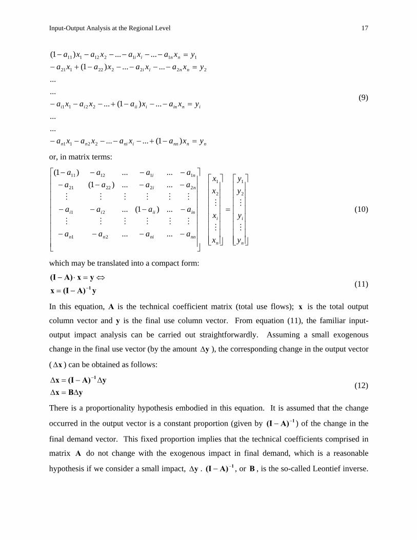
Input-Output Analysis at the Regional Level 17
nnnnininn
ininiiiii
nnii
nnii
yxaxaxaxa
yxaxaxaxa
yxaxaxaxayxaxaxaxa
=−+−−−−−
=−−−+−−−
=−−−−−+−=−−−−−−
)1(............
...)1(.........
......)1(......)1(
2211
2211
222222121
111212111
(9)
or, in matrix terms:
⎥⎥⎥⎥⎥⎥⎥⎥
⎦
⎤
⎢⎢⎢⎢⎢⎢⎢⎢
⎣
⎡
=
⎥⎥⎥⎥⎥⎥⎥⎥
⎦
⎤
⎢⎢⎢⎢⎢⎢⎢⎢
⎣
⎡
⎥⎥⎥⎥⎥⎥⎥⎥⎥
⎦
⎤
⎢⎢⎢⎢⎢⎢⎢⎢⎢
⎣
⎡
−−−−
−−−−
−−−−−−−−
n
i
n
i
nnninn
iniiii
ni
ni
y
y
yy
x
x
xx
aaaa
aaaa
aaaaaaaa
2
1
2
1
21
21
222221
111211
......
...)1(...
......)1(
......)1(
(10)
which may be translated into a compact form:
yA)(IxyxA)(I
1−−=
⇔=⋅− (11)
In this equation, A is the technical coefficient matrix (total use flows); is the total output
column vector and y is the final use column vector. From equation (11), the familiar input-
output impact analysis can be carried out straightforwardly. Assuming a small exogenous
change in the final use vector (by the amount
x
yΔ ), the corresponding change in the output vector
( ) can be obtained as follows: xΔ
yBxyA)(Ix 1
Δ=ΔΔ−=Δ −
(12)
There is a proportionality hypothesis embodied in this equation. It is assumed that the change
occurred in the output vector is a constant proportion (given by ) of the change in the
final demand vector. This fixed proportion implies that the technical coefficients comprised in
matrix do not change with the exogenous impact in final demand, which is a reasonable
hypothesis if we consider a small impact,
1A)(I −−
A
yΔ . , or B , is the so-called Leontief inverse. 1A)(I −−

Input-Output Analysis at the Regional Level 18
Each of its elements traduces the value of output i required directly and indirectly to deliver
one additional monetary unit to j’s demand (Miller, 1998).
ijb
7 In analytical terms, j
iij y
xb
∂∂
= . If
we sum up each column of this inverse matrix, we obtain , which are the output
multipliers.
∑=
• =n
iijj bb
1
8 These represent the value of the economy-wide output required directly and
indirectly to deliver one additional monetary unit to j’s demand. In other words, they measure
the impact over all the economy caused by a change in the final demand for output j.
The Leontief inverse can also be approximated through a mathematical series expansion. Given
that the technical coefficients matrix verifies the conditions of being “(…) a square matrix in
which all elements are nonnegative and less than one, and in which all column sums are less than
one” (Miller, 1998, p. 53), the inverse can be expanded using the following power
series expression:
A
1A)(I −−9
++++++=− − k321 AAAAIA)(I (13)
This expression highlights the presence of different types of effects (initial, direct and indirect
effects)10 caused by an exogenous change in final demand (Miller, 1998). Inserting equation
(13) into (12), we obtain:
( )yAyAyAyAyx
yAAAAIxk32
k32
Δ++Δ+Δ+Δ+Δ=Δ
Δ++++++=Δ (14)
From this equation we can see that, when the vector of final demand changes, this causes an
initial effect of the same amount on the output vector, given by the first term: . To satisfy
these new productions, industries will have to buy some new inputs, given by - these are
the direct effects. The remaining terms capture the indirect effects caused by the fact that the
yΔ
yAΔ
7 It should be noted that output i may either be domestically produced or imported. Also, the initial impact over product j is not exclusively directed to domestic production, but is indifferent to the geographic origin of the product. Further on this paper, we will present alternative multipliers which measure specifically the impact over domestic production. 8 Other types of multipliers can be computed. For example, if we weight the elements of the inverse matrix by appropriate employment coefficients, we can deduce employment multipliers, measuring the impact on employment, created by exogenous changes in final demand. For further details see, for example, Miller (1998), pp. 61-64. 9 This results is similar to that of ordinary algebra, according to which a power series of infinite terms like
++++++ krrrr 321 is equal to ( ) 11 −− r , given that 10 ≤≤ r . 10 Sometimes, initial and direct effects are lumped together and considered both as direct effects. This is why Leontief inverse is also known by the matrix of direct and indirect requirements.

Input-Output Analysis at the Regional Level 19
production of those new inputs also requires intermediate consumption of additional inputs. Of
course, as it happens in any power series expansion, as the exponent increases, the corresponding
effect decreases, implying that the latter indirect effects will be necessarily smaller than the
former indirect effects that are, in turn, smaller than the direct effects.
Some hypotheses are implicit in the kind of reasoning exposed above, frequently pointed out as
limitations of input-output (mainly when it is used as a forecast model): first, the elements of
matrix are assumed to be time-invariant, meaning that the underlying technology is constant.
Obviously, this is a restrictive assumption in long-run forecast applications of the model, making
it more suitable to short-run uses. Secondly, it is assumed that the aij are the same, irrespective
of the scale of production (constant returns to scale), which implies that scale economies are not
taken into account; thirdly, the assumption of constant aij also implies that we are dealing with a
fixed proportion technology; in fact, if we consider two inputs, i and k, to produce output j, the
proportion in which they are used is given by
A
,kj
ij
j
kj
j
ij
kj
ij
aa
xaxa
zz
== which is constant, since the
technical coefficients are also constant (Miller and Blair, 1985). Finally, the production capacity
is supposed to be unlimited; when the final use of some product increases, it is assumed that the
output of this product and the others will be able to meet the additional direct and indirect
requirements, without any capacity restrictions. With the aim of overcoming these shortcomings
of the model, several developments have been introduced into the basic formulation: for
instance, dynamic models that consider varying technical coefficients and models that include
capacity restrictions. Yet, in the present work, the basic formulation will be used, since
forecasting impacts is not our primary objective.
3. Regional input-output models Although originally conceived for national-wide applications, input-output models have been
applied to sub-national geographic units since the second half of the last century. According to
Miller and Blair (1985), there are two specific features associated to the regional dimension
which make evident and necessary the distinction between national and regional input-output
models. First, the technology of production of each region is specific, and it may be close or, on

Input-Output Analysis at the Regional Level 20
the contrary, very different from the one that is registered at the national input-output table; for
example, the age of regional industries, the characteristics of input markets or the education level
of the labor force are important factors that may influence the regional technology of production
to deviate from the national one. Secondly, the smaller the economy under study, the more it
depends on the exterior world, making more relevant the exported and imported components of
demand and supply, respectively. It should be noted that these components correspond not only
to international trade, but also to the trade between the region and the rest of the country to
which the region belongs.
In this section we aim to review the main contributions in regional input-output modeling. The
following models are distinguishable by four main criteria:
- the number of regions taken into account: single-region or many-region models.
- the recognition (or not) of interregional linkages;
- the degree of detail implicit in interregional trade flows (which is related to the degree of
detail demanded for the input-output data) and
- the kind of hypotheses assumed to estimate trade coefficients.
We will begin by presenting the single-region model (section 3.1) that has a similar structure to
the nation level input-output model presented in the previous section. Then, we proceed to those
models that try to capture not only intra-regional transactions, but also the interconnections
between regions. Of these, we begin by reviewing Leontief’s intranational model (section 3.2),
that consists of a very primary type of regional input-output model, since the only spatial effect it
recognizes concerns the one-way effect of national changes over regional output. As will be
seen, spillover and feedback regional effects are not considered by this model. The remaining
models (sections 3.3. to 3.5) seek to account for inter-spatial effects. Yet, they differ in the
degree of detail used in the specification of interregional trade flows. Besides, the two multi-
regional models (Chenery-Moses and Riefler-Tiebout) are distinguished by the hypotheses they
assume to determine trade coefficients. One common feature of the last three regional models is
the fact that trade coefficient stability is assumed. We will provide special attention to this
aspect in section 3.6.

Input-Output Analysis at the Regional Level 21
3.1 Single-region model
The aim of single-region input-output models is to evaluate the impact on regional output caused
by changes in regional final demand. The starting point for a single-region model is, obviously,
a single-region input-output table. In similar manner to the nation-level table, the single-region
input-output table may be presented in two different versions: as a total-use table or as an intra-
regional flow table.11 The correspondence between the structure of these two regional tables and
the national tables presented above is straightforward. If we consider that, in figure 1, the row of
imported products includes also imports from other regions of the same country and the vector of
final demand comprises also considers exports to the rest of the country, then this table
represents a single-region input-output table, with total use flows. Correspondingly, if we take
similar considerations over the table in figure 2 (concerning imports and exports) and consider
additionally that the intermediate and final use flows include only regionally produced inputs,
then figure 2 can be converted into a single-region input-output table, with intra-regional flows.
These two types of data arrangement originate two different single-region models: (1) total-use
single-region model and (2) intra-regional single-region model.
The development of the total-use single-region model follows closely the development of the
nation-level input-output model made in the previous section. Let us use the superscript r to
denote a regional variable; thus, for example is the amount of output i available in region r
(including international and interregional imports), represents regional final demand for
product i (including the one that consists of imported products) and denotes the total amount
of input i used in the production of output j in region r (including imported inputs as well).
Then,
rix
riy
rijz
rj
rijr
ij xz
a = is the regional technical coefficient, defined in a similar way as the national one.
This indicates the amount of input i necessary to produce one monetary unit of output j in region
r. In should be stressed out that all the possible geographic origins of input i are being included
in the calculation of this coefficient, meaning that comprises product i produced in region r
but also produced in other regions or even abroad, since it is traded in region r. Using the
regional variables instead of the national ones, we can write an equation similar to equation (1):
rijz
11 In the context of regional models the word “intra-regional” is used with the same meaning as the word “domestic”, in the nation-level models.

Input-Output Analysis at the Regional Level 22
......21ri
rin
rii
ri
ri
ri yzzzzx ++++++= (15)
Considering the regional technical coefficient rj
rijr
ij xz
a = , this equation becomes:
ri
rn
rin
ri
rii
rri
rri
ri yxaxaxaxax ++++++= ......2211 (16)
The compact matrix representation correspondent to the previous equation (considering one
equation like this to each of the n products) is:
r1rr
rrr
y)A(Ixyx)A(I
−−=
⇔=⋅− (17)
This solution allows us to quantify the impact over the total output available at region r caused
by a change in regional final demand. Following the development of the national model, we may
write: r1rr y)A(Ix Δ−=Δ − (18)
It should be noted that this impact is not limited to the region itself; instead, some of the impact
measured by this equation is felt outside the region, via effect on imported products (included in
the values of vector ). Yet, it is possible to estimate the impact over regional production from
the total-use model. If we pre-multiply both sides of the previous equation by , in which
is a diagonal matrix
rx
( cI ˆ− )c 12 of import propensities, we obtain the impact on regional production. A
careful analysis of the reasonability of this procedure is made in Sargento (2009).
Let us now consider an intra-regional input-output table (similar to the one in figure 2) as the
starting point to the input-output model development. The major difference relies on the type of
coefficient used; instead of the regional technical coefficient, a supply coefficient that indicates
the amount of regionally produced input i necessary to produce one monetary unit of output j in
region r is considered. This is called an intra-regional input coefficient, sometimes simplified to
regional input coefficient (Miller and Blair, 1985). Let denote the amount of regionally
produced input i used in the production of output j in region r. Then, the intra-regional input
coefficient may be computed as:
rrijz
rj
rrijrr
ij ez
a = , in which denotes regional production of product
j. Considering additionally as the region’s final demand towards product i produced in region
rje
rif
12 We will use a to note a diagonal matrix composed by the elements of column vector . ˆ a

Input-Output Analysis at the Regional Level 23
r (including regional requirements as well as exports for any other regions, national or foreign),
the solution of the single-region input-output model with intra-regional flows follows the same
procedures as before. In matrix terms, Let us use the notation:
• - a matrix composed by intra-regional input coefficients ; rrA rrija
• - the vector of output produced in region r; re
• - the vector of regional final demand towards products produced in region r. rf
Then, the final equation of the single-region model with intra-regional flows is:
( )rrrr
r1rrr
fBefAIe
=
−=−
(19)
Applying impact analysis to this model, we get: rrrr ΔfBΔe = (20)
The intra-regional inverse matrix measures the impact of changes in final demand for
regional products over regionally produced output. The fundamental differences between this
equation and equation (18) are: (1) the impact is quantified over regional production ( ), while,
in equation (18), the impact is estimated over total output available in the region ( ); (2) the
initial change refers to final demand for regionally produced products, , whereas, in equation
(18), the initial change refers to regional final demand (for both regional production and imports:
) and (3) the inverse matrix is obtained from intra-regional coefficients, whereas in equation
(18), the inverse matrix is obtained from (total) regional technical coefficients.
rrB
rerx
rΔf
rΔy
Of course, the practical application of the single-region model with intra-regional flows requires
that the researcher has previous access to the vector of regional outputs, which generally occurs,
and also to the matrix of intra-regional flows and to the vector of final demand, . These
two latter statistics are much more difficult to obtain. As noted in Miller (1998), “To generate
these kinds of data through a survey, respondents must be able to distinguish regionally supplied
inputs from imported products” (p. 87). This is valid for firms, when asked about their
intermediate consumption patterns, but also for final users. It is obvious that the fundamental
problem in conducting such a survey is not the usually mentioned time and cost restrictions, but
rather the fact that the respondents may not know the answer. In fact, most of industrial units buy
their inputs in wholesale traders which, in turn, sell a mix of regional and imported products. It
rrZ rf

Input-Output Analysis at the Regional Level 24
should be stressed that imported products, in a regional context, involve also products from other
regions. Thus, it is very difficult for firms to answer whether a specific input i was imported or
not, from other countries or other regions. For obvious reasons, the problem of not knowing the
origin of the products is even more manifest in what respects to final consumers. That being the
case, a set of hypotheses is usually applied in order to estimate from a regional technical
coefficients matrix . In Sargento (2009), it is demonstrated that if consistent hypotheses are
used in both types of single-region models (total-flow and intra-regional flow), the results
provided by both are equivalent and the total-flow single-region model is capable of measuring
the same kind of impacts as those derived from the intra-regional single-region model.
rrArA
Regardless of the type of flows being considered, the single-region model has a crucial limitation
of theoretical nature: it consists of the fact that it ignores the effects caused by the linkages
between this region and the others (in the same country and abroad). Exports are considered as
exogenous variables. However, in reality, when a new final demand occurs in one specific
region, the impact doesn’t confine itself to its boundaries; instead, in order to satisfy the new
final demand, the first region will need to import goods and services from the other regions, for
use in intermediate consumption. This effect is indeed of growing importance, given the
increasing economic integration between the different countries and regions (Van der Linden and
Oosterhaven, 1995). One of two fundamental inter-spatial effects, which are neglected by the
single-region model, are the spillover effects, which account for the change in the production of
other regions caused by input purchases made by the first region (to answer its own additional
needs). The remaining regions, in turn, may need to import inputs from other regions (probably
including the first region) to use in their own production. These demands introduce the concept
of interregional feedback effects, that are caused by the first region itself, through the
interactions it performs with the remaining regions (Miller, 1998).
3.2 Leontief’s intranational model.
Leontief developed his first spatial input-output model in 1953. This was a very simple model,
both in analytical as well as in data requirements. In his intranational model, also called a
balanced regional model, he combined the traditional input-output analysis with the awareness
that “some commodities are produced not far from where they are consumed, while the others
can and do travel long distances between the place of their origin and that of their actual

Input-Output Analysis at the Regional Level 25
utilization” (Leontief, 1953, p. 93). In order to account for such spatial interaction, yet in a crude
manner, he begins by distinguishing two classes of commodities: “regional” and “national.”
“Regional” commodities are supposed to be regionally balanced, which means that all the
regional production is consumed in the same region. Examples of such goods might be: utilities,
personal services and real estate (Miller and Blair, 1985). Conversely, “national” commodities
are those which are “...easily transportable...” (Leontief, 1953, p. 94) and in which production-
consumption balance occurs only at the national or even at the international level. Products like
cars or clothes can fit into this category. This implies that one region may have production in
excess of some “national” product, generating exports to the rest of the country, or instead, it
may have a deficit, which leads to imports from the rest of the country. The model only
computes net trade flows, rather than gross exports and gross imports, and it does not determine
the region of origin (destination) of the imports from (exports to) the rest of the country. This is
the reason why the author prefers to label this model intranational, instead of interregional.
The ultimate aim of this model is to determine the regional impact of an exogenous change in the
final demand for “national” and / or “regional” products (Miller and Blair, 1985). The following
set of hypotheses support the development of the model:
• There are n products, divided in “regional” (from 1 to h) and “national” (from h+1 to n),
according to the previous definitions; this classification is known a priori.
• There are k regions.
• The technical coefficients, j
ijij x
za = , are known and the same technological matrix is
used for all regions and for the nation as a whole.
• The national and regional outputs, as well as the national and regional final demands, are
known a priori (for both “national” and “regional” commodities); “national”
commodities are marked with the subscript N and “regional” commodities are marked
with the subscript R; let the national outputs and final demand be represented by the
following vectors. It should be emphasized that these subscripts refer to types of products
and not to geographic locations:

Input-Output Analysis at the Regional Level 26
⎥⎦
⎤⎢⎣
⎡=
⎥⎥⎥⎥
⎦
⎤
⎢⎢⎢⎢
⎣
⎡
=
⎥⎥⎥⎥
⎦
⎤
⎢⎢⎢⎢
⎣
⎡
=
⎥⎦
⎤⎢⎣
⎡=
⎥⎥⎥⎥
⎦
⎤
⎢⎢⎢⎢
⎣
⎡
=
⎥⎥⎥⎥
⎦
⎤
⎢⎢⎢⎢
⎣
⎡
=
+
+
+
+
N
RNR
N
RNR
yy
yyy
xx
xxx
n
h
h
h
n
h
h
h
y
yy
y
yy
x
xx
x
xx
2
1
1
1
2
1
1
1
At the regional level we have precisely the same set of variables; as usual, a superscript r is used
to denote a regional variable.
• The market share of each region in providing each of the “national” products, r
r NN
N
xx
τ = , is
also given a priori and it is assumed to be constant, i.e., “the regional output of these
commodities is assumed to expand and contract proportionally with the change in
national demand” (Polenske, 1995).
Using these hypotheses, equation yxA)(I =⋅− , introduced previously, yields for the impacts
for the economy as a whole. Only, in this case, matrix may be looked as a composition of
four different matrices, taking into account the classification of commodities into “regional” and
“national”:
A
⎥⎦
⎤⎢⎣
⎡=
NNNR
RNRR
AAAA
A (21)
Making use of the previously defined composed vectors and , the solution of the model can
be expressed, in this case as (Miller and Blair, 1985):
x y
( )( )
( )( ) ⎥
⎦
⎤⎢⎣
⎡⎥⎦
⎤⎢⎣
⎡−−−−
=⎥⎦
⎤⎢⎣
⎡
⇔⎥⎦
⎤⎢⎣
⎡=⎥
⎦
⎤⎢⎣
⎡⎥⎦
⎤⎢⎣
⎡−−−−
−
N
R
NNNR
RNRR
N
R
N
R
N
R
NNNR
RNRR
yy
AIAAAI
xx
yy
xx
AIAAAI
1 (22)
This equation quantifies the nation-wide impact on the total output of each type of products,
caused by an exogenous change in the demand for “the outputs of one or more national sectors
and/or one or more regional sectors” (Miller and Blair, 1985, p. 87). The Leontief inverse may
also be seen as decomposed in two, in which the upper part represents the direct and indirect

Input-Output Analysis at the Regional Level 27
requirements of “regional” products and the lower part represents the direct and indirect
requirements of “national” products (Leontief, 1953):
⎥⎦
⎤⎢⎣
⎡=
⎥⎥⎥⎥⎥⎥⎥⎥⎥
⎦
⎤
⎢⎢⎢⎢⎢⎢⎢⎢⎢
⎣
⎡
=
+
++++++
+
+
+
N
R
BB
B
nnhnnhnn
nhhhhhhh
hnhhhhhh
nhh
nhh
bbbbb
bbbbbbbbbb
bbbbbbbbbb
121
11112111
121
21222121
11111211
(23)
Until now, no spatial dimension was included in the model. To do so, we need to consider the
market share of each region in providing each of the “national” products, N
rNr
N xx
=τ . From this, it
follows that, for each region r , the output of the “national” commodities is a function of the
national output of the same commodities:
NrN
rN xx τ= (24)
or, in matrix terms, , in which represents a diagonal matrix with the market shares
for each “national” product in the main diagonal.
NrN xτx ˆ= τ
Focusing on “regional” commodities, we can define the regional output from the demand
perspective. However, we must be aware that “regional” inputs may be required for the
production of both “regional” and “national” industries operating in that region. As a result, the
regional output of “regional” commodities is given by:
rR
m
hj
rjRj
h
j
rjRj
rR yxaxax ++= ∑∑
+== 11 (25)
which, using the relevant sub-matrices defined in (21), and considering also equation (24),
corresponds to:
( )( ) ( )( ) ( ) r
R1
RRNRN1
RRrR
rR
1RR
rNRN
1RR
rR
rR
rNRN
rRRR
rR
rNRN
rRRR
rR
yAIxτAAIx
yAIxAAIx
yxAxAI
yxAxAx
−−
−−
−+−=
−+−=
+=−
++=
ˆ
(26)
This equation means that the regional output of “regional” commodities is a function not only of
the regional demand for these commodities, but also of the national output for “national

Input-Output Analysis at the Regional Level 28
commodities.” However, according to equation (22), national output for “national commodities”
is, in turn, a function of national demand for both types of products. Thus, ultimately, this model
quantifies the regional impact caused by changes in the national demands for both products,
allocating “the impacts of new and demand to the various sectors in each region” (Miller
and Blair, 1985, p. 88).
Ry Ny
In spite of its pioneering character in trying to capture spatial interactions and its ease
application, the results from the empirical applications of this model were not satisfactory,
because it relies on the use of net trade flows leading to the underestimation of the interregional
feedback effects previously referred (Polenske and Hewings, 2004). The importance of these
effects will be discussed later on.
3.3 The Isard IRIO (interregional input-output model)
An interregional input-output model was proposed by Isard (1951). The review of this model
will be presented following Miller (1998)’s example for a two-region system: region r and region
s. Let us consider that each region has n industries and each industry produces only one product
(and vice-versa). Then, the domestic production of product i in region r, may be written in the
demand perspective, as:
( ) ( ) ri
rsin
rsi
rsi
rrin
rri
rri
ri fzzzzzze ++++++++= ...... 2121 (27)
This equation embraces intra-regional intermediate uses of input i and also inter-regional sales of
the same input for intermediate consumption, as well as for final uses (these are included in the
aggregate which contains: private and government consumption, and investment in the
region, exports for other regions for final uses and total exports to foreign countries). It should
be noted that only the demand addressing regional production is included in the amount .
rif
rif
Using the supply perspective, the production of product j in region r is given by:
( ) ( ) rj
rj
srnj
srj
srj
rrnj
rrj
rrj
rj wmzzzzzze +++++++++= ...... 2121 (28)
In this equation, represents international imports used as intermediate consumption in the
production of j.
rjm
The two preceding equations make clear that the interregional input-output model is inherently
an intra-regional flow input-output model; the fundamental difference between this model and
the intra-regional single-region input-output model described before consists of the fact that the

Input-Output Analysis at the Regional Level 29
former model takes into account the spillover and feedback effects, through the inclusion of one
(or more) additional region in the system.
The next step consists in developing the model, which requires the use of the following
coefficients:
rj
rrijrr
ij ez
a = , for region r and sj
ssijss
ij ez
a = , for region s, as intra-regional input coefficients;
sj
rsijrs
ij ez
a = and rj
srijsr
ij ez
a = , as interregional trade coefficients.
For example, represents the amount of input i from region r necessary per monetary unit of
product j produced in region s.
rsija
Using these coefficients, equation (27) can be written as: r
isn
rsin
srsi
srsi
rn
rrin
rrri
rrri
ri feaeaeaeaeaeae ++++++++= ...... 22112211 (29)
This equation may be expressed in matrix terms, given: rrA , as the intra-regional input coefficient matrix for region r (generic element: ); rr
ija
ssA , as the intra-regional input coefficient matrix for region s (generic element: ); ssija
rsA , as the interregional trade coefficient matrix with generic element ; rsija
srA , as the interregional trade coefficient matrix with generic element ; srija
rf and , as the final demand vectors for production of region r and s, respectively. sfre and , as the output vectors for region r and s, respectively. se
Hence, the following system of equations yields for the two regions:
ssssrsr
rsrsrrr
f)eA(IeAfeA)eA(I=−+−
=−− (30)
If we define a matrix as a partitioned matrix composed of four sub-matrices defined
previously in this model:
ISA13
⎥⎦
⎤⎢⎣
⎡=
sssr
rsrrIS
AAAA
A ;
13 superscript IS stands for Isard’s model

Input-Output Analysis at the Regional Level 30
if, additionally, we aggregate the output and final demand vectors as follows:
⎥⎦
⎤⎢⎣
⎡=
s
r
ee
e and , ⎥⎦
⎤⎢⎣
⎡=
s
r
ff
f
the matrix system for the two-region interregional model assumes the following expression:
fe)A(I IS =⋅− (31)
Thus, the solution to this model is given by:
fBef)A(Ie IS1IS =⇔⋅−= − . (32)
From this equation, one can perform economic impact analysis, making:
ΔfBΔeΔf)A(IΔe IS1IS =⇔⋅−= − (33)
This final equation is similar to the one found in the single-region model with intra-regional
flows (equation 20), but the similarity is a little misleading, since the degree of detail and
complexity in this model is much higher. Now the economic impact is determined not only in
terms of the different regions, but also in terms of the different industries, because the
interregional trade flows comprised in the model not only specify the region of origin and the
region of destination, but also the industry of origin and of destination (Isard, 1951). In other
words, the model assumes that “(…) any given commodity produced in a region is distinct from
the same good produced in any other region” (Toyomane, 1988, p. 16). Besides, the previously
referred spillover and feedback effects are now accounted for; any change in the final demand of
one region causes effects on the others and these return to the first region, through the
interregional linkages specified in the model. The magnitude of the interregional feedback
effects may be isolated. Following Miller (1966), and going back to equation (30), the outputs of
each region may be written in terms of the final demands and , as follows: rf sf

Input-Output Analysis at the Regional Level 31
[ ]
[ ]
[ ][ ]
[ ][ ]⎪⎪⎪
⎩
⎪⎪⎪
⎨
⎧
−−−
+−−−−=
−−−−
+−−−=
⎩⎨⎧
+−=−+−−−−−
⎩⎨⎧
=−+−−−−−−−
⎩⎨⎧
=−+−+−−−+−=
⎪⎩
⎪⎨⎧
=−+−
=−−
−−
−−−
−−−
−−
−−
−−
−−
−−
s1rs1rrsrss
r1rrsr1rs1rrsrsss
s1ssrs1sr1ssrsrr
r1rs1ssrsrrr
sr1rrsrsssrs1rrsr
ssssr1rrsrsrs1rrsr
ssssr1rrsrs1rrsr
r1rrsrs1rrr
ssssrsr
rsrsrrr
fA)A(IA)A(I
f)A(IAA)A(IA)A(Ie
f)A(IAA)A(IA)A(I
fA)A(IA)A(Ie
ff)A(IAe)A(IA)A(IA
f)eA(If)A(IAeA)A(IA
f)eA(If)A(IeA)A(IAf)A(IeA)A(Ie
f)eA(IeAfeA)eA(I
(34)
Let us analyze the economic significance of this equation, taking for example, the expression of
region s’s output: this is determined by the total requirements needed to satisfy the final demand
within the region and also by the total requirements needed to satisfy the final demand in region
r. Let us look at these two components with greater detail, starting with the requirements to
provide . In an intra-regional single-region model with no interregional linkages, the total
effect on region s would be given by the traditional inverse
sf
( ) 1ssAI −− . However, this is not the
case here. Therefore, we must consider also the interregional feedback effects. First, region s
will require inputs from region r; this link is expressed by the interregional trade matrix . In
turn, region r will answer this new demand through its total requirements matrix: .
However, we are interested in estimating the effects on region s’s output. The additional
production in r will be reflected in s, through the demand for inputs expressed by . Thus, the
interregional feedback effect felt in region s is given by
rsA
( ) rs1rr AAI −−
srA
( ) rsrrsr AAIA − . The other component
of implicit in equation (34) results from the requirements necessary to provide, . First,
region r will suffer an intra-regional effect given by,
se rf
( ) r1rr fAI −− . Because of this, region r will

Input-Output Analysis at the Regional Level 32
import some inputs from region s; this effect is felt on region s by the amount, .
This can be seen as a new demand in s, that causes effects similar to those explained before,
given by the direct and indirect requirements matrix:
( ) r1rrsr fAIA −−
[ ] 1rs1rrsrss A)A(IA)A(I −−−−− .
From the previous exposition, the following question may arise: what is the magnitude of the
interregional effects, or, in other words, what is the magnitude of the error caused by neglecting
these effects? To answer this question, let us suppose that a change in final demand for regional
products has occurred, either originating in region r or in region s: rΔf . The effect of this in
region r is given by: . If no interregional feedback
effects were taken into account, the corresponding effect would be: . Then,
the difference between these two effects reflects the amount due to interregional feedback
effects. This is, still, an empirical issue. In some cases, the error may be small, as in the tests
made in Miller (1966). In others, the error is quite significant, as happened in the empirical
application for the interregional model with eight-region and twenty-three industries developed
by Greytak (1970). Greytak (1970) concluded that, when feedback effects are taken into
consideration, the resulting multipliers are about 14% larger than when these effects are
neglected. In essence, these two empirical results depend heavily on the data and, in particular,
on the degree of intraregion-self-sufficiency and on the size of the regions under study.
[ r1sr1ssrsrrr ΔfA)A(IA)A(IΔe −−−−−= ]( ) r1rrr ΔfAIΔe −−=
Of course, the degree of complexity involved in interregional input-output model has a reflection
on the demand for data to implement it: it is extremely data demanding, especially when it comes
to interregional trade flows. In fact, if it is often difficult to gather data on trade flows from one
region to the others, and it is even more difficult to collect these data specifying the industry of
origin and the industry of destination of those flows.
It should be also noted that, in the example used to present this model, only two regions were
considered. In this case, the compact matrix is composed of 4 matrices, each
with dimension (being n the number of industries and of products). If three regions were
considered, then matrix would be composed of 9
⎥⎦
⎤⎢⎣
⎡=
sssr
rsrrIS
AAAA
A
nn×ISA nn× matrices. Generalizing, if k regions
are considered, matrix is a composition of ISA 2k nn× matrices. Then, it is clear that the

Input-Output Analysis at the Regional Level 33
amount of data required to implement such a model increases quickly with the number of regions
being studied (Miller and Blair, 1985).
Finally, it should be emphasized that the use of equation (33) implies the supposition of constant
elements in matrix (Isard, 1951). In this system, these elements comprise two kinds of
coefficients: intra-regional input coefficients and trade coefficients (Oosterhaven, 1984). The
stability supposition is, therefore, extended to the trade coefficients, which may be an even more
restrictive assumption than the one attributed to constant technical coefficients. The implications
of the interregional trade stability will be the focus of section 3.6.
A
3.4 Chenery-Moses MRIO (multiregional input-output model)
Given the difficulty in gathering the data required to implement Isard’s model, it has seldom
been applied. With the aim of overcoming this drawback, Chenery (1953) and Moses (1955)
developed the first version of a multi-regional input-output model that used the following
simplification: interregional trade flows are only specified by region of origin and region of
destination, thus ignoring the specific industry (or final consumer) of destination.
The data requirements to this model imply that the researcher has previous access to four sets of
data. The first consists of an Origin-Destination (O-D) matrix for each and every product,
depicting intra and interregional shipments of the outputs of that product. Such matrix can be
illustrated in figure 3.
Figure 3: Intra and interregional shipments of product i.
DESTINATION
r s
r rrix rs
ix
OR
IGIN
s srix ss
ix
SUM riR s
iR
In this matrix, , for example, represents the amount of product i produced and consumed in
region r and represents the amount of product i shipped by region s to region r, without
rrix
srix

Input-Output Analysis at the Regional Level 34
specifying the type of buyer in the region of destination (it may be used by any industry or even
to final users). The column total of this matrix will be denoted by: , for the first column,
representing the total amount of product i available in region r, except for foreign imports; ,
for the second column, representing the total amount of product i available in region s, except for
foreign imports.
riR
siR
The second set of information consists of an interindustry flow matrix for each region. For
example, for region s, we will need a matrix sZ • , in which each element describes “the
value of purchases by each industry in a region from each industry in the nation as a whole
during some base period” (Moses, 1955, p. 805). In other words, all geographic origins of input i
are being considered, except for foreign countries.
sijz •
Finally, it is necessary to know, in advance, the vectors of regional final demand for each region
(in which, for example, denotes final demand for product i in region r, including all regional
sources of i) and also the vectors of regional production in each region ( stand for regional
production of product i in region r).
riy
rie
The starting equations for the development of this model are similar to those presented in the
previous section. The balance equations state “that the output of each industry in each region is
equal to its sales to all industries and final demand sectors in all regions” (Moses, 1955, p. 804).
Considering, as before, a system of two regions (r and s) with n industries and n products each,
we may write:
( ) ( )( ) ( sr
isrin
sri
sri
ssi
ssin
ssi
ssi
si
rsi
rsin
rsi
rsi
rri
rrin
rri
rri
ri
fzzzfzzze
fzzzfzzze
+++++++++=
+++++++++=
......
......
2121
2121
)
, (35)
for all 14.,,1 ni =
Given that intra-regional flows such as or are not easy to obtain through direct
observation, some hypotheses are considered in order to use more accessible data. The first
fundamental hypothesis consists of the introduction of the so-called trade coefficients. Using the
information of the O-D matrix depicted before, and dividing each element of the first column by
rrijz rr
if
14 As it happens in the original presentation of the model, it is assumed that the two-region system is closed, thus having no interaction with the rest of the world, either through international imports or exports. This is clear in Moses (1955), in which the author states: “Let us assume a closed economy divided into r regions which are open to one another for trade in n homogeneous commodities” (p. 827). For this reason, international exports are not included in equation (35).

Input-Output Analysis at the Regional Level 35
its column total, we obtain the proportions of the product available in region r that is provided by
the region itself and by the other region. Analytically, we make: ri
rrirr
i Rx
t = and ri
srisr
i Rx
t = .
Because these coefficients are computed dividing each element of the O-D matrix by the column
total, the MRIO model is sometimes called a column-coefficient model (Polenske, 1995).15
The essential hypotheses underlying MRIO is the assumption of the same trade coefficient
applies to all the different uses in the destination region. In other words, this means that if, for
example, , meaning that 40% of all the product i available in region s comes from region
r, the assumption implies that for all intermediate and final uses of product i in region s, 40%
comes from region r and only 60% is provided by region s itself
4,0=rsit
16 (Toyomane, 1988). This is
often called the import proportionality assumption (Riefler and Tiebout, 1970). Moses (1955)
recognizes that it is an imperfect assumption; yet, it is adopted, given the fact “that it is
impossible to implement statistically a model which applies separate trading patterns to each
industry” (Moses, 1955, p.810).
Introducing these trade coefficients into equations (35), and making use of the known
information on the matrices sZ • and rZ • and on the vectors of regional final demand, we obtain:
( ) ( )( ) ( r
isri
rin
sri
ri
sri
ri
sri
si
ssi
sin
ssi
si
ssi
si
ssi
si
si
rsi
sin
rsi
si
rsi
si
rsi
ri
rri
rin
rri
ri
rri
ri
rri
ri
ytztztztytztztzte
ytztztztytztztzte
+++++++++=
+++++++++=••••••
••••••
......
......
2121
2121
) (36)
for all .,,1 ni =
The other type of coefficient used in this model consists of technical coefficients. In this
particular case, the inter-industry flows (described in matrices sZ • and rZ • ), record the total
15 The column-coefficient multi-regional model, developed by Chenery and Moses, is the most popular MRIO and the pioneering one; yet, other MRIO models, that computed trade coefficients in a different manner, were proposed thereafter: namely the row-coefficient model (in which trade coefficients are obtained dividing each element of the O-D matrix by the row total) and the gravity-trade model, also called Leontief-Strout Gravity model (in which trade coefficients are computed on the basis of a gravitational formula to calculate trade flows, being these a function of total regional outflows, total regional inflows and the cost of transferring the goods from one region to another). Details on these alternative multi-regional models can be found in Polenske (1970a), Polenske (1970b), Polenske (1995) and Toyomane (1988). Empirical tests applied to these models, with the aim of assessing their capacity in estimating regional outputs and interregional trade flows, revealed that, concerning the row coefficient, the results are not satisfactory (Polenske, 1970b); in the case of the gravity-trade model, this was only applicable when access to previous interregional trade flows existed; otherwise, the model had to be solved iteratively, and it didn’t converge (Polenske, 1995). 16 Once again, we stress the fact that, in this model, foreign imports are excluded from this assumption.

Input-Output Analysis at the Regional Level 36
inputs used by each industry in each region, regardless of the regional provenance of those inputs
(assuming a closed economy, thus with no imports from abroad).17
Let represent the total amount of product i used as an input by industry j in region s. Symbol
is used to represent the summation of all the geographical origins of input i, except for foreign
countries. Then,
sijz •
•
sj
sijs
ij ez
a•
• = is the technical coefficient for region s and it represents the amount
of product i necessary to produce one unit of industry j’s output in region s, considering the
inputs provided by all the regions in the system (Moses, 1955). Using these coefficients, the
system of equations (36) becomes:
( ) ( )( ) ( r
isri
rn
rin
sri
rri
sri
rri
sri
si
ssi
sn
sin
ssi
ssi
ssi
ssi
ssi
si
si
rsi
sn
sin
rsi
ssi
rsi
ssi
rsi
ri
rri
rn
rin
rri
rri
rri
rri
rri
ri
yteateateatyteateateate
yteateateatyteateateate
+++++++++=
+++++++++=•••••
••••••
......
......
22112211
22112211
)
(37)
for all .,,1 ni =
In this equation, technology and trade are treated as separate factors, thus representing an
advantage of this model over the IRIO model (Toyomane, 1988). In fact, given that the factors
that influence technology and trade are most likely different, it seems more appropriate to treat
the two components separately.
Generalizing for all regions and products, we may write the structural form of the model in
matrix terms. To do so, Let us consider:
- the input matrices: , of generic element ; , of generic element ; rA • rija• sA • s
ija•
- the trade matrices T , for each pair of origin and destination, with all the products being
traded represented in the main diagonal; for example: ;
ˆ
⎥⎥⎥⎥⎥
⎦
⎤
⎢⎢⎢⎢⎢
⎣
⎡
=
rsn
rs
rs
t
tt
000000000000
ˆ 2
1
rsT
17 Instead of considering that the known information on inter-industry flows concerns to flows coming from the whole nation, as it is done in Miller (1985), Miller (1998) and Moses (1955) we might consider that the researcher has previous access to a technological matrix, i.e., a matrix with total flows (inputs coming from the whole nation and also from abroad). In this case, the trade coefficients would have to be computed in a consistent manner, dividing each element of the O-D matrix, not by its column total, but by the total output available at the correspondent region (which includes foreign imports).

Input-Output Analysis at the Regional Level 37
- the vectors of final demand in region r ( ) and in region s ( ). Since, in this model, the
trade flows don’t specify the type of user at the destination, this implies that final demand of
each region may as well be partially supplied by imports from the other region.
ry sy
Joining these data together, the structural form of this two-region model, in the demand
perspective, is given by:
sssrsrssssrrsrs
srsrrrssrsrrrrr
yTyTeATeATeyTyTeATeATe
+++=
+++=••
••
(38)
If we take the following partitioned matrices18 and vectors: ;
; and , the final equation, in a compact form is:
⎥⎦
⎤⎢⎣
⎡=
•
•
s
rCM
A00A
A
⎥⎦
⎤⎢⎣
⎡=
sssr
rsrr
TTTT
T ⎥⎦
⎤⎢⎣
⎡=
r
r
ee
e ⎥⎦
⎤⎢⎣
⎡=
s
r
yy
y
TyeTAe CM += (39)
This equation can be used to perform economic impact analysis, in similar fashion to equation
(33), in IRIO. Given any change in y , caused either by changes in one or more product final
demands of region r or region s, the new output vector is
yTΔ)TA(IΔeTy)eTA(ITyeTAe 1CMCMCM −−=⇔=−⇔+= (40)
It should be noted that the inverse matrix relating the new final demand with the new output
vector is now . This implies that the multiplier effect, quantified by the column
sum of this matrix, can be understood as a two-stage effect (Miller, 1998): first, matrix T , with
the trade coefficients, operates the distribution of the new final demands in each region by the
suppliers in each region; then, multiplying this by , it provide the total impacts
(direct and indirect) on the regional industries.
T)TA(I 1CM −−
1CM )TA(I −−
3.5 Riefler-Tiebout’s bi-regional input-output model
Riefler and Tiebout (1970) also made an important contribution to regional input-output models,
proposing a specific formulation of an interregional input-output model, suited for the particular
situation in which the system is composed by two-regions (plus the rest of the world) and the
researcher has previous access to an imports matrix and an exports matrix for one of those
18 superscript CM stands for Chenery-Moses model.

Input-Output Analysis at the Regional Level 38
regions. It is clear by now that this model requires more survey-based data than the Chenery-
Moses multi-regional model. In Riefler and Tiebout (1970), the authors used the example of a
bi-regional system composed of the states of California and Washington, since there was an
exports matrix and an imports matrix for Washington. These two matrices depicted, for each
input and for each consuming industry and final demand sector, the percentage of the input that
came from / went to abroad (including here the other region and foreign suppliers / receivers). In
this case, the fundamental problem would be confined to partitioning this matrix into imports
from (exports to) California and imports from (exports to) the rest of the world (Harrigan, et al.
1981).
The structural equations of the model are similar to those presented in Isard’s IRIO model.
Considering again two regions, r and s, and using the previously defined matrices of coefficients,
the structural equations could be written as in equation (41):
ssssrsr
rsrsrrr
f)eA(IeAfeA)eA(I=−+−
=−− (41)
The contribution of Riefler and Tiebout’s model concerns the way in that they specify the
interregional trade coefficients and . Making use of the existing data, they assume a
compromise between the ideal interregional trade coefficients proposed by Isard and the
simplified trade coefficients used by Chenery and Moses. In the Isard’s IRIO model, was
obtained dividing the observed flow by the observed value, . However, as noted earlier,
this demands a degree of detail in the data that is seldom available. In the Chenery-Moses
model, was replaced by the multiplication of the trade coefficient by the technical coefficient
for region M: ; in this case,
rsija sr
ija
rsija
rsijz s
je
rsija
sij
rsi
rsij ata •⋅= s
i
rsirs
i Rx
t = , which implies the use of the imports
proportionality assumption. Using the imports matrix for Washington, Riefler and Tiebout
demonstrate that this assumption is far from being verified in reality; in fact, different industries
present different input import propensities. One of the main reasons behind this is the fact that
inputs and outputs are classified under non-homogeneous groups of products. Thus, they
propose a procedure in which this assumption is avoided.
From the import matrix, available for Washington (region r), they were able to compute the
percentage of the total imports of input i (coming from California - region s - and from abroad)

Input-Output Analysis at the Regional Level 39
that was used in the intermediate consumption of industry j. In order to obtain the interregional
trade coefficient , the only hypotheses to assume was that a constant share of those imports
came from region s – this share was computed for each input i making use of a set of trade
related statistics, including the US Census of Transportation.
srija
19 Similarly, from the export
matrix, they could calculate the percentage of the total exports of input i which was destined to
the consumption of industry j (both in California and in foreign countries). Given this, could
then be computed assuming that a constant share of these exports was destined to region s
(California). This export share was estimated using the same set of statistical sources as for the
import share. These interregional trade coefficients were then introduced in equation (41),
allowing the deduction of the inverse matrix expression, as presented in IRIO:
rsija
20
fBef)A(Iefe)A(I
RT1RT
RT
=⇔⋅−=
=⋅−−
(42)
As it became clear from the previous exposition, the practical utility of this model is limited to
situations in which exist both an import matrix and an export matrix to one of the regions under
study. Besides, the model implies that one region relies on the information obtained for the other
region in terms of trade. Thus, even when such information is available, the first concern of the
researcher should be to question the accuracy of the pre-existing matrices. The difficulties in
conducting surveys to assess the proportion of imported products used as intermediate
consumption have already been mentioned in the exposition of the single-region model. Mainly,
they have to do with the fact that, usually, the sources of information – responding enterprises –
cannot distinguish their inputs into imported and regional ones. Yet, is should be recognized that
it is easier to obtain an answer to the question “Are the inputs imported or regional?” than to the
question “Are the inputs imported or regional and where do the imported inputs come from?”
The latter question is implicit in the trade data required by the Isard model, whereas the former is
implicit in the trade data demanded by the Riefler-Tiebout model. Hence, this model seeks an
approximation of Isard’s trade coefficients, using less demanding survey information and
complementing it by the use of alternative sources as the Census of Transportation. For the
export matrix, the problems in gathering such information are similar, or even more serious. The
fact is that firms know the proportion of output they export, but they usually cannot distinguish 19 See Riefler and Tiebout (1970) for further details. 20 In equation (42), RT stands for Riefler and Tiebout.

Input-Output Analysis at the Regional Level 40
the specific destination user of their exports, in terms of industries or final users (since the goods
may be shopped to a wholesaler who determines the final destination). In conclusion, while
theoretically interesting, this model has a considerable practical disadvantage over the Chenery-
Moses model.
3.6 Trade coefficient stability
As we have seen, the previous interregional and multiregional input-output models may be used
for impact analysis caused by changes in regional final demands. In these kinds of applications,
besides the usual assumption of constant technical coefficients, an additional supposition is
implicit, namely that the trade coefficients are stable21 (Riefler and Tiebout, 1970). This means
that when a shift in final demand occurs, the trading patterns remain unaltered. This is, in fact, a
much stronger assumption than the classical assumption of constant technical coefficients
(Batten and Boyce, 1986). Moses (1955) evaluates this supposition, analyzing the economic
forces behind the trading patterns and the conditions that must hold for their stability. Trade
flows are influenced essentially by “cost-price relationships and regional capacities for
production and distribution” (Moses, 1955, p. 810). As such, trade coefficients are stable if the
following conditions hold: regional costs of production are constant, unit costs of transportation
are fixed and the capacity of production can be easily increased. For the first two conditions,
these are very restrictive, but they are generally adopted in input-output models, thus being a
general limitation of these models and not a specific problem of MRIO models. As for the third
condition, its reasonableness depends essentially on the elasticity of production factors, in
particular, labor. From this point of view, it would be preferable to apply this model to long-run
periods, since it would facilitate the adjustment of production capacities. However, this would
increase the probability of regional technological changes, affecting not only the stability of trade
coefficients, due to changes in relative costs of production, but also the typically assumed
stability of technical coefficients. Moses (1955) concludes arguing that the MRIO model is best
suited to short-run impact analysis, given that the factors of production are below full
employment situation.
21 In Isard’s model, trade coefficients are not explicit in the model. However, assuming intra-regional and interregional input coefficients as constant corresponds to the assumption that, not only the input structure is constant, but also the percentage that comes from the region itself and from other regions.

Input-Output Analysis at the Regional Level 41
4. Obtaining the data for regional input-output models: table construction As any model requires its own database, the regional input-output models implementation also
implies the previous existence of the corresponding input-output tables. Yet, whereas at the
national level the input-output tables are regularly provided by the official statistics, according to
standardized rules, the same does not apply to the regional dimension. For that reason, the
construction of regional input-output tables has been, by itself, one of the most debated themes in
regional literature. The researchers have sought for a compromise on the adoption of common
rules which allow for the comparability of regional economic structures in space and time
(Hewings and Jensen, 1986).
According to Jensen (1990), it is possible to distinguish four stages in what is concerned to the
history of regional input-output table construction: (1) in the first stage, national coefficients
were used directly, without any adjustments, in the regional input-output table; (2) in the second
stage, those national coefficients were adjusted in order to reflect some specific regional
characteristics; (3) the third stage, named the “classical era of regional input-output” (Jensen,
1990, p.11) was dominated by the supporters of survey-based tables, which were elaborated by
research teams and implied a vast field work; in this era, “the achievement of the highest quality
table was regarded in itself as an end” (p. 11); (4) the end of the classical era was determined by
the high requirements in terms of human labor, logistics, money, etc, demanded by survey tables.
Today we are at the fourth stage, in which hybrid tables, that combine direct information with
values obtained by non-survey techniques, are seen as the most adequate alternative. Survey,
non-survey and hybrid techniques will be discussed with further detail in the subsequent
sections.
4.1 Survey table
As the name suggests, survey tables are assembled on the basis of the direct surveys made to
firms, consumers and government institutions, and also on the basis of experts’ judgments about
each sector. These are commonly seen as the most accurate tables, since they attempt to reflect
all the specific characteristics of the regional economy. However, besides the already mentioned
problem of being very time and cost demanding, survey techniques involve other pitfalls.
Several types of errors can emerge immediately in the process of gathering the data: for example,
errors arising from incorrect definition of the sample, poor design of questionnaires, hiding of

Input-Output Analysis at the Regional Level 42
information or lack of concern in answering the questionnaires (Jensen, 1980). Even with
exactly the same set of data, different research teams can achieve different input-output tables,
because compilation procedures are not unique (for example, there are different methods of
making the reconciliation between sales and purchases data)22. Moreover, when non coincident
data are provided by different sources – by statistical methods based on surveys on the one hand,
and by experts’ judgments, on the other hand – the difficulty is to decide which one of these
sources is more reliable (see Jensen, 1990). Besides these problems, survey methods involve
another difficulty: as referred before, sometimes the questions included in the questionnaires
require very detailed information to which some respondents may not be able to answer (for
example, if the inputs used are imported or not and from where they are imported). This being
the case, even the official agencies collecting statistics, when they compute regional input-output
tables, are often forced to use some hypotheses in order to complement the information they
cannot obtain directly from surveys, thus using a hybrid method.
4.2 Non-survey and hybrid techniques
Non-survey techniques applied to regional input-output tables can be generally defined as a set
of procedures that aim to fill the components of a regional table on the basis of values comprised
in a similarly structured national table (Jensen, 1990). These techniques are also called top-down
methods, since they use the values of the whole nation as a starting point and then apply specific
regional indicators to regionalize them. The indicators used depend on the available data at the
regional level, but usually they embrace employment and income data.
Obviously, non-survey techniques include a vast set of methods, which is not homogeneous.
Yet, regardless of the specific method to be used, the accuracy of non-survey regional input-
output tables is highly determined by the following issues (Lahr, 1993): industrial mix,
technology and external trade. Each of these elements assumes a different influence in the
table’s accuracy. For example Park, et al. (1981) made some tests in order to study the effect on
the input-output table created by errors in technology and in trade estimation. They conclude
that errors in estimating the regional inputs coefficients are more determined by errors in
22 Reconciliation problems occur whenever there is no coincidence with the values obtained by the seller perspective (values at the rows) and the ones assembled through a user perspective (at the columns) (Lahr, 1993).

Input-Output Analysis at the Regional Level 43
regional trade estimation than by errors in technical coefficients. Let us explain each of these
elements with greater detail.
Differences between the regional industrial mix and the national one may create errors in the
tables derived by non-survey methods, since national structures are applied to regional industries
in which the proportion of each sub-industry is different from the national one (some sub-
industries that exist at the national level may even be inexistent at the some specific region).
However, this is a problem that may be partially solved if the researcher uses a high degree of
disaggregation when regionalizing the national table (Park, et al., 1981; Goldman, 1969). Today
this does not constitute an operational problem, given the high computational capacities to deal
with highly detailed tables.
Technology and external trade issues have been treated by the literature in a very confusing
manner. As an example, Czamanski and Malizia (1969) state that one of the most important
sources of error caused by the use of the national coefficients is the “relative importance and
structure of foreign trade” (p. 65). This makes clear that technology and trade are mixed topics.
We recognize that, in regional input-output models, these two issues are always interconnected;
yet, we will try to treat them as two separate items in what concerns the development of input-
output tables.
In non-survey regional input-output tables, the technical coefficients matrix is sometimes set
equal to its national counterpart. This is called the “national technology assumption.” It is
convenient to recall what these technical coefficients mean: they express the amount of input i
per unit of output j, regardless of the geographic origin of input i. This means that the national
interindustry transactions matrix to be used as a starting point has to be a total flow matrix,23
thus including both nationally produced and imported inputs. So, the implicit hypothesis is that
technology, in the production function sense, is spatially invariant within the same country (Lahr,
1993). Given that a high disaggregation is in fact used in the industry classification, this
hypothesis is not very restrictive (Madsen and Jensen-Butler, 1999). It is rather acceptable to
assume that some specific industry (taken at a very refined level of disaggregation) uses the same
productive recipe in region r or in any other region of the same country. Moreover, some
empirical exercises have concluded that this assumption does not cause major errors in the table.
23 In the Portuguese National Accounts, the national matrix is, in fact, a total flow matrix. But this is not the rule; in some countries, as in the USA, the published national matrices exclude foreign imports. This implies a previous adjustment to the national matrix before regionalizing it. This will be further discussed in Sections 5.2 and 5.3.

Input-Output Analysis at the Regional Level 44
As an example, Boomsma and Oosterhaven (1992) compared the regional technical coefficients
obtained through this national technology assumption with regional technical coefficients
obtained via direct information and concluded that “the national technology assumption produces
a close approximation, even for subsectors that are specific for the region at hand” (p. 278). This
is an argument in favor of non-survey techniques as far as technology assumptions are
concerned. Of course, this is an empirical issue, which depends greatly on the specific national
and regional economies under study. Harrigan et al. (1980), for example, performed an
empirical comparison between a survey-based regional technological matrix (existing for
Scotland) and the corresponding non-survey matrix, computed using the technology of the
United Kingdom. Contrarily to the case mentioned before, the results of this study found large
differences between these two matrices; thus, in this case, the use of the national technical
coefficients leads to substantial biases in regional impact analysis. Still, the national technology
assumption continues to be a crucial hypothesis to assume in regional table construction, since
the alternative survey regional tables seldom exist.
Using the national technology assumption, the regionalization of the interindustry transactions
table is usually made using the industry’s total intermediate consumption in each region as the
key regionalizing indicator. This means that only the purchases are regionalized. In other
words, each column of the national interindustry transactions table is divided in as many
columns as the number of regions. This is called a columns-only or purchases-only
regionalization (Oosterhaven, 1984). Assuming two regions, r and s, the resulting regional
columns depict how much of the intermediate consumption of industry j is used in region r and
in region s (being both regional columns decomposed in several inputs). The spatial origin of the
inputs is not specified. An alternative way of regionalizing the national interindustry
transactions table, presented by Oosterhaven (1984), would be rows-only: each national row, that
describes the intermediate sales of inputs i, would be divided by regions. In this case, the
resulting regional rows would specify how much of the intermediate sales of industry i would be
made by region r and by region s (being both decomposed by the several consuming industries).
The spatial destination of these sales would not be specified. This alternative is less used than
the first, mainly because the available regional data that serve as an indicator to regionalize are
frequently of the “purchase” kind: usually, the researcher has access to regional values of

Input-Output Analysis at the Regional Level 45
intermediate consumption by industry, but not to regional values of intermediate sales by
industry.24
Last, but not least, the accuracy of non-survey tables is determined by the methods used to
estimate a region’s external trade. We have to distinguish the two types of external trade
concerning a regional economy: (1) imports and exports between it and other countries and (2)
imports and exports between it and other regions (Isserman, 1980). The first kind of external
trade is not really a problem, because this is usually available from official statistical sources.
The difficulty is in estimating interregional trade flows. This is an old and remaining problem,
as suggested by Czamanski and Malizia (1969): “Foreign trade is an especially sensitive issue at
the regional level because of the notorious lack of reliable data on interregional flows” (p. 65).
Despite the non-survey techniques chosen to estimate interregional trade, this problem comprises
two distinct questions:
(1) How to estimate the interregional trade flows necessary to fulfill an Origin-Destination
matrix to each of the products being considered? In other words, only the commodity
shipments from and to each region are computed. This is an unavoidable concern to
anyone who intends to assemble a multi-regional input-output table. In fact, we have seen
in section 1.3 that, among the three many-region models (Isard, Chenery-Moses and
Riefler-Tiebout models), the Chenery-Moses model was the one that implied the
minimum amount and detail of data, concerning interregional trade. Such data consisted
precisely of an Origin-Destination matrix to each of the products being considered,
depicting the shipments from the region of origin to the region of destination. Even if the
investigation falls upon a single-region table, it is still necessary to estimate exports from
the region to the rest of the country, as part of the demand directed to the region, and
imports coming from other regions, given that these are part of the supply available at the
region25.
(2) How to estimate the interregional (and international) imports comprised in the regional
technological matrix, in order to achieve intra-regional input coefficients? In other words,
24 In Oosterhaven (1984) another alternative is presented, that combines the information of the columns-only with the rows-only method of regionalization. The regional table obtained in this way is called a Full Information table. Besides being more data demanding, this method implies the reconciliation between the two types of information. 25 As it will be seen latter, in single-region tables, usually net interregional flows are estimated, instead of gross exports to the rest of the country and gross imports from the rest of the country.

Input-Output Analysis at the Regional Level 46
this means: how to determine the proportion of the inputs used that comes from the
region itself? This may be seen as an optional task in the table construction stage. Given
that non-survey techniques are used, the same hypotheses that can be used to estimate
intra-regional input coefficients in the table construction stage may, as an alternative, be
applied in the model phase, starting from a total use technological matrix. This is
demonstrated in Sargento (2009).
Among survey and non-survey methods, there is a wide range of techniques that combine direct
information with estimated values: these are generically labeled as hybrid techniques (Lahr,
1998). In reality, it is very difficult to find tables that are exclusively survey or non-survey. This
is because purely survey tables are too expensive to construct and purely non-survey tables are
too inaccurate for conducting input-output analysis (Dewhurst, 1990). According to Round
(1983), “The terms non-survey and survey suggest the existence of two well defined and
mutually exclusive groups, but in practice virtually all input-output tables are hybrid tables
constructed by semi-survey techniques, employing primary and secondary sources to a greater or
lesser extent” (p. 190). Anyway, it is generally agreed that the more direct information that is
incorporated in the table, the more accurate it tends to be. Of course, direct information implies
higher costs, which leads to a cost-benefit analysis where, according to West (1990), the
equilibrium occurs when the marginal benefit of substituting estimated for direct information in
the table equals the marginal cost of obtaining this direct information. This being the case, the
introduction of direct information must be selective. For example, Lahr (1993) considers that
this direct information should always be obtained, at least, for sectors in which the region is
highly specialized or in sectors in which technological differentiation is more probable, namely,
resource-based industries and residual categories, because these are more likely to have a
regionally differentiated industrial mix26 (example: “Manufacture of other non-metallic mineral
products”).
4.3 Matrix adjustment methods: the particular case of RAS
Belonging to the vast family of hybrid methods are matrix adjustment methods. Matrix
adjustment methods are applied whenever the researcher wants to find the values to fill in a 26 Yet, it should be noted that, when the model is based on a fine product disaggregation, these residual categories tend to disappear or to become insignificant, such that their influence to the global accuracy of the model is almost null.

Input-Output Analysis at the Regional Level 47
specific matrix on the basis of another matrix, which can be considered as a good indicator to the
first one, and with regard to specific prior restrictions (Harrigan, 1990). For example, these
methods can be applied to estimate a regional technical coefficients matrix, which will be the
target matrix, on the basis of: (1) the national technical coefficients matrix or a regional technical
coefficients matrix for a comparable region and (2) some partial information about the target
matrix, usually concerning its column and row totals. In this case, the adjustment is made across
space. But we can similarly apply a matrix adjustment method to update any technical coefficient
matrix (regional or national) existing for an earlier year to a more recent year – here, the
adjustment is made across time (Miller and Blair, 1985). Either the adjustment is made across
space or across time, the general principle behind matrix adjustment methods “consists into
finding what is the matrix which is closest to an initial matrix but with respect of the column and
row sum totals of the second matrix” (de Mesnard, 2003, p. 1).
Matrix adjustment methods are intensively used in several types of applications, ranging from
the assemblage of National Accounts to many other fields in which the missing data can be
presented in a matrix form: international and interregional trade, migration flows, transportation
flows, and so on (Lahr and de Mesnard, 2004; Jackson and Murray, 2004). Additionally, matrix
adjustment methods comprise a vast set of algorithms. An exhaustive review of these algorithms
is beyond the objectives of the present work.27 We will focus only on the most popular matrix
adjustment method: RAS. Among other attributes, which will be mentioned below, RAS
presents two main practical advantages over competitive algorithms: it is a very simple technique
and it requires a minimum amount of data (Lahr and de Mesnard, 2004; Mohr, Crown and
Polenske, 1987). Besides, a number of the empirical studies (for example: de Mesnard, 2003;
Oosterhaven, et al., 1986 and Jackson and Murray, 2004), that assessed the relative performance
of alternative matrix adjustment methods conclude that, most of the times, RAS produced the
best results, measured by the proximity between the estimated matrix and a known target
matrix.28
27 Recently, matrix adjustment methods have gained a renewed interest. Thus, there are some recent papers that make a quite complete review and discussion of the alternative matrix adjustment algorithms. Some examples are: Lahr and de Mesnard (2004), de Mesnard (2003), de Mesnard (2006) and Jackson and Murray (2004). 28 Yet, these authors also stress the fact that the empirical results cannot be definitively generalized, because they depend heavily on the particular features of the matrices to be adjusted and also on the measures used as matrix comparison methods.

Input-Output Analysis at the Regional Level 48
Let us review the application of RAS, through the following example of adjustment across space:
the researcher wants to find a matrix of regional technical coefficients for region 1, , through
the adjustment of a previously known matrix of regional technical coefficients existing for
the same year, for a comparable region: region 0. To do so, the researcher has previous access to
four pieces of information:
1A0A
• The matrix of regional technical coefficients , which is the starting matrix; 0A
• Total output by industry for region 1: ; 1jx
• Total intermediate sales of each commodity i, for region 1: ∑=•j
iji zz 11 ; this corresponds
to the sum of all elements of row i in the matrix of intermediate transactions . Z
• Total intermediate consumption for each industry j, for region 1: ; this
corresponds to the sum of all elements of column j in the intermediate transactions Z .
∑=•i
ijj zz1
The RAS procedure is carried out iteratively, in several steps. First, it is assumed that technical
coefficients are equal in both regions: 10 AA = . Under this hypothesis, the intermediate
transactions matrix for region 1 would be obtained multiplying these technical coefficients by the
correspondent industry outputs. In matrix terms, this can be written as: 10xAZ ˆ=I (43)
in which represents a first estimate (denoted by index I) of the intermediate transactions
matrix for region 1, with generic element
IZ
( )Iijz1 , and represents a diagonal matrix with total
industry output for region 1 in the main diagonal. illustrates the intermediate transactions
that would be observed in region 1 if there were no differences between technological structure
of region 1 and region 0 (Jackson and Murray, 2004). The row sums of this matrix,
, must be compared with the actual, known, row sums . To do so, let us
define the quotient
1x
1jx IZ
( ) ( )∑=•j
Iij
Ii zz 11 1
•iz
( )Ii
iIi
z
zr
1
1
•
•= . The numerator of this quotient comprises known information,
whereas the denominator is a result of the assumed hypothesis about the regional technical

Input-Output Analysis at the Regional Level 49
coefficients. Hence, quotient is an indicator of the sign and value of the error implicit in the
hypothesis of equal regional technical coefficients. If, for example, , this means that all
the elements of row i were assumed greater than they should be, since . If we
multiply all these elements by , we will obtain a new set of technical coefficients which, after
being multiplied by industry outputs, will sum exactly . In matrix terms, and making the
same to each row, this corresponds to generating a new technical coefficients matrix as:
Iir
1<Iir
( ) 11•• > i
Ii zz
Iir
1•iz
( ) 0ˆ ArA II = (44)
in which represents a diagonal matrix with quotients in the main diagonal. From
technical coefficients matrix , we can now compute a new intermediate transactions matrix:
Ir Iir
( )IA
( ) ( ) 11 xAZ ˆIII= (45)
Given the way in which it was obtained, the row sums of this new intermediate transactions
matrix must now equal the known values . However, the column sums 1•iz ( ) ( )∑=•
i
IIij
IIj zz 11
must be also compared with the known values . This is why RAS is called a bi-proportional
adjustment method: both row sums and column sums must be respected. Let us define the
quotient
1jz•
( )IIj
jIIj
z
zs
1
1
•
•= . This quotient is used to uniformly adjust all the elements of column j, in
order to obtain a new set of technical coefficients which, after being multiplied by industry
outputs will sum exactly . In matrix terms, this corresponds to: 1jz•
( ) ( ) IIIIIII sArsAA ˆˆˆ 0== (46)
After computing the new intermediate transactions matrix29, ( ) ( ) 11 xAZ ˆIIIII= , the consistency
between the corresponding row and column totals and the known values has to be checked again.
New quotients and are computed and the process is repeated iteratively until convergence ir js
29 In the above exposition the iterative procedure is applied to the technical coefficients matrix ( ), whilst quotients r and s are computed from the intermediate consumption flow matrix (
AZ ). This is done in order to facilitate the
understanding of the meaning of quotients r and s and it is correct since the multiplication of diagonal matrices is commutative, thus: . sZrsxArxsAr ˆˆˆˆˆˆˆˆ ==⋅

Input-Output Analysis at the Regional Level 50
between the obtained and known totals is achieved. In the several applications of RAS, it has
been verified that the process usually converges meaning that quotients and in iteration
are closer to one that in iteration t . The iterative process should stop when the difference
between the known margins and the estimated ones is very small. One concrete reference
number is presented by Miller and Blair (1985) in the example used by these authors: the
difference should not exceed 0.005 (Miller and Blair, 1985, p. 286).
ir js
1+t
Although quotients and have been presented in the context of the algebraic exposition of
the RAS technique, some authors consider that they may be interpreted as economic effects
(Miller and Blair, 1985). This is the case of Stone,
ir js
30 the precursor of this technique which
considered that the uniform row adjustments (through quotient ) are a result of a substitution
effect, while the uniform column adjustments (through quotient ) are a result of a productivity
effect. Substitution effects may occur due to changes in the relative prices of inputs or merely
because of the emergence of new substitute inputs. As an example, if plastic materials substitute
for metallic materials, this will be reflected in the increase of technical coefficients in the row
corresponding to plastic inputs (which will have a quotient greater than one) and on the
reverse effect in the metallic inputs row (with less than one). The productivity effect results
from changes in productivity of industries, due to technological progress or change in labor
skills, which generate a reduction in intermediate consumption, compensated by an increase in
value added. In this case, there is a reduction in all the technical coefficients of the column
corresponding to the industry in which productivity has changed and this is reflected by a
quotient less than one (Miller and Blair, 1985). This interpretation of RAS, though
interesting, has been questioned by several authors.
ir
js
ir
ir
js31 Conversely, it is commonly argued that
RAS can be seen as a merely mathematical formula, since it is proven to correspond to the
solution of a problem of minimization of information bias (de Mesnard, 2003; Miller and Blair,
1985; Oosterhaven, Piek and Stelder, 1986; Harrigan, 1990), such as:32
30 Stone, R. 1961. “Input-Output and National Accounts”. Paris: Organization for European Economic Cooperation. Referred in Miller and Blair (1985). 31 For example, Lahr and de Mesnard (2004), have shown that the absolute values of and cannot be interpreted, but rather their relative values. For further details, please refer to the paper.
ir js
32 The analytical demonstration that RAS is a solution of a constrained problem of minimization of information bias can be found, for example, in Miller and Blair (1985), pp. 309-310 or in de Mesnard (2003), p. 7.

Input-Output Analysis at the Regional Level 51
111
111
0
11
..
ln1
jji
iji
ij
ijj
ijj
ij
i j ij
ijij
a
zxaz
zxazts
aa
aIMinij
•
•
==
==
⎟⎟⎠
⎞⎜⎜⎝
⎛=
∑∑
∑∑
∑∑
(47)
This means that the target matrix is generated in order to be as close as possible to the prior
matrix and, at the same time, respect the row and column sum constraints (Jackson and Murray,
2004). Hence, RAS tends to preserve, as much as possible, the structure of the initial matrix.
Regardless of the way in which RAS can be understood, the fact is that it has been widely
applied, with quite good results, with special emphasis in input-output studies. The main
theoretical advantages of RAS are listed by Oosterhaven, et al. (1986): first, unlike other
adjustment methods (example: minimization of square differences), RAS does not give a major
weight to a few large differences, neglecting many small differences; secondly differences are
weighted by their significance in the updated matrix (as it can be seen by coefficient in
problem (47), while other methods use no weight value or instead use the value of the initial
matrix; finally, RAS produces positive values in all the cells of the matrix to be adjusted, where
there is positive value in the starting matrix, which is an advantage over other methods that
generate surprising and economically meaningless negative coefficients (this occurs in non-
biproportional approaches, for example, the minimization of square differences) (Lahr and de
Mesnard, 2004). However, some disadvantages are also commonly pointed out to RAS, namely:
(1) it is not capable of dealing with negative values in the matrix to be adjusted (this can be seen
in equation (47), which, due to the presence of the logarithmic function, is not defined for
negative values); (2) every null cell in the initial matrix continues to be null in the final matrix
(Oosterhaven et al., 1986); this can be seen as a drawback in some cases. For example, if
industry j in region 0 uses no input i as intermediate consumption, thus presenting a null
technical coefficient, RAS forces the same to happen in region 1, which sometimes may not be
the case.
1ija
The application of RAS (or other biproportional adjustment methods) as part of a hybrid method
in input-output table assemblage often involves the use of some known a priori information on
the matrix to be found. For example, if the researcher knows, in advance, that for some industry

Input-Output Analysis at the Regional Level 52
j in region 1 the consumption of input i is null (conversely to what happens in region 0) this
information should be incorporated in the adjustment method. In this case, this could be done
setting the specific technical coefficient to zero in the initial matrix; as it was mentioned before,
this will remain zero until the process converges. If the researcher has previous knowledge of
the specific value (different from zero) of intermediate consumption flow for industry j and some
input i then he/she should set that specific cell to zero and subtract the known value from the
corresponding row and column totals. At the end of the RAS procedure, that known value is
placed back in the appropriate cell (Lahr and de Mesnard, 2004). Dewhurst (1990) examined the
performance of RAS technique, with and without the introduction of known direct information
about the target matrix. His empirical exercise consisted in updating a 1973 regional matrix (for
Scotland) to year 1979, for which a survey table existed. Comparing the output multipliers
obtained from the RAS adjusted table (with no incorporation of known a priori information)
with the actual output multipliers, this author concluded that the percentage errors are quite
small. The same exercise was repeated, increasingly inserting more known interior information
in each step. The results showed that the introduction of superior information “does on average
improve the multipliers derived from the estimated table” and that “there appears to be
decreasing returns to additional superior information” (Dewhurst, 1990, p. 85).
4.4 Evaluating the accuracy of estimated input-output tables.
Regardless of the specific technique (non-survey or hybrid) that has been used in the
construction of an input-output table, it is important to assess, whenever possible, the accuracy or
degree of exactness possessed by the obtained table (Jensen, 1980). However, three questions
immediately arise:
(1) Is there any objective standard agiants which the estimated table can be compared?
(2) What is the concept of accuracy that should be privileged in such comparison?
(3) Which quantitative measures should be used to make such comparison, in practice?
The first question comprises two different issues: first, if for example the estimated input-output
table is for a specific region, there may not be another input-output table for the same region;
secondly, provided that such comparative table exists, it is necessary to evaluate if it is
sufficiently reliable to serve as a benchmark. In fact, the true input-output table for a specific

Input-Output Analysis at the Regional Level 53
economy may never be known. As we have mentioned before (in section 4.2), even in the so-
called survey tables, assembled by direct observations, several types of errors can emerge. Thus,
it is very difficult to define a consensual standard against which constructed tables should be
compared. As an alternative, Jensen (1980) proposes an indirect evaluation of the accuracy of
the table, assessing its ability in generating known variables, for example, using the constructed
table for year t to forecast known values of industry outputs for year t+1.
When assessing accuracy in the context of input-output studies, we should be aware of the
different perceptions it can involve. Jensen (1980) provided a major contribution to the
clarification of the concept of accuracy in regional input-output studies. First, it is important to
distinguish the accuracy of the input-output table (called A-type accuracy) from the accuracy of
the input-output model (B-type accuracy). “A-type accuracy refers to the degree to which an
input-output table represents the ‘true table’ for the economy” (Jensen, 1980, p. 140). B-type
accuracy involves a broader concept, referring “to the exactness with which the input-output
model reflects the realism of the operation of the regional economy” (Jensen, 1980, p. 141). To
implement an input-output model, some assumptions must be added to the data comprised in the
base input-output table. For example, the use of fixed technical coefficients implies the
assumption that no economies of scale exist. Thus, it is important to be aware of these
assumptions when applying an input-output model and to check whether they are acceptable in
the specific situation at hand. Probably, for a significant increase in output levels, there may be
considerable economies of scale, which may cause errors in the model. Hence, B-type accuracy
is determined by the degree to which such assumptions are met by the real economy under study.
The problem is that, generally, the researcher does not have such enough knowledge about the
operation of the regional economy, implying that information on B-type accuracy is difficult to
obtain (Hewings and Jensen, 1986).
A-type accuracy, in turn, may be interpreted in two ways: partitive and holistic accuracy (Jensen,
1980). Partitive accuracy refers to a cell-by-cell accuracy. In this sense, the input-output table is
seen as a number of separate components. Thus, an input-output table is accurate in a partitive
sense, if each and every cell accurately approximates the corresponding cell in the standard table.
Jensen (1980) argues very clearly that partitive accuracy is impossible to achieve in constructed
regional input-output tables, given the common situation of regional data availability; moreover,
it is not cost effective, because a large percentage of the cells of the table are not significant to

Input-Output Analysis at the Regional Level 54
the integrity of the table as a whole. Some empirical results reinforce the previous idea. Jensen
(1980) refers to the conclusions of experimental work which revelaed “that more than fifty
percent of the smaller coefficients of a table can be removed (set equal to zero) before a ten
percent error appears in input-output multipliers” (p. 147). Additionally, this author stresses the
fact that, even when the researcher establishes partitive accuracy as the ultimate goal, the
difficulty emerges when it is necessary to assess such accuracy. The fact is that tests often made
to infer partitive accuracy in non-survey regional input-output tables are erroneous, since the
constructed tables are compared against survey tables that, as noted earlier, are not error free in a
partitive sense.
Instead of partitive accuracy, Jensen (1980) advocates the use of holistic accuracy as a criterion
to assess A-type accuracy. He defines holistic accuracy of an input-output table as “the ability to
represent the size and structure of the economy in general terms” (Jensen, 1980, p. 143). This
means that in holistic accuracy, more important than the absolute values of each cell are their
relative magnitudes in relationship with each other; for example, more important than accurately
assessing the value of each intermediate consumption flow is the correct assessment of the
cost structure of industry j in region r, which implies an accurate assessment of the relative
values of each intermediate consumption flow in column j. It is true that, if an input-output table
verifies partitive accuracy, then it follows that “the table as a whole will reflect the true table
with a high degree of accuracy” (Jensen, 1980, p. 142). This means that partitive accuracy in the
table implies holistic accuracy. Conversely, the presence of holistic accuracy doesn’t guarantee
that all the cells of the table are accurate in a partitive sense; particularly it does not imply
partitive accuracy in those cells that are less significant in the economy in study. Thus, the
accuracy of the table as a whole is usually greater than the accuracy of each of its cells. This is
because holistic accuracy focuses attention on the larger or most important elements of the
economy being studied (Hewings, 1983). This concept of accuracy has guided some projects of
table assemblage through hybrid methods (for example: see West, 1990, and Lahr, 1998). In this
context, direct information should be used for certain cells, identified as critical to the model
accuracy. If the model is directed towards a specific industry, for example, the table assembling
team should pay special attention to the cells that determine the accurate representation of that
industry; in general terms, these are the ones located at that column’s industry and the ones with
which it maintains strong inter-industrial relationships (West, 1990). Several methods have been
rijz

Input-Output Analysis at the Regional Level 55
developed to identify important sectors in the model construction stage. An important sector, in
the table construction sense, is defined by Lahr (1998) as “a sector for which superior data will
significantly improve nonsurvey model accuracy” (p. 4). This author’s paper and the other
studies referenced therein provide a comprehensive review of these methods, that are beyond the
scope of the present work.
Miller and Blair (1985) illustrate the distinction of partitive and holistic accuracy through the
following example (pp. 286-288): an hypothetical technical coefficients matrix for a specific
target year is estimated on the basis of a similar technical coefficients matrix existing for a base
year, through the application of the RAS technique. At the end of the iterative adjustment
process, the estimated matrix is compared with the actual, known matrix, in two distinct ways:
(1) comparing each estimated technical coefficient with the corresponding real value – which
means that partitive accuracy is being evaluated and (2) comparing the output multipliers
obtained from the estimated technical coefficient matrix with the output multipliers obtained
from the real technical coefficient matrix – in this case, what is being evaluated is how well the
technical coefficients perform in practice, and this depends on how accurately they depict the
structure of the economy (accuracy in the holistic sense). Using specific quantitative measures
to make such comparisons (discussed later on in this section), the results show that: the RAS
adjusted table is not accurate in a partitive sense, since the average percentage error is around
64%; however, the corresponding output multipliers are very close to the real ones (the
maximum percentage error is 1,27%), which reflects a high holistic accuracy of the estimated
table. Obviously, in consideration of typical applications of input-output tables, the researcher
should be more concerned with the accuracy of the output multipliers, than with the accuracy of
each individual technical coefficients.
It must be noted that the choice of criterion about A-type accuracy has implications on B-type
accuracy. Given that the input-output model is based on the input-output table, part of the
accuracy of the model is obviously determined by the accuracy of the table. Thus, beyond Type
B errors, an input-output model based on a table that verifies accuracy in a holistic sense will be
better suited to illustrate the functioning of the most important sectors of the economy (Jensen,
1980). Thus, the results provided by such input-output model should be cautiously interpreted,
“within the unknown but probably generous limits of accuracy and precision suggested by the
concept of holistic accuracy” (Hewings and Jensen, 1986, p. 317). Even if the researcher aspires

Input-Output Analysis at the Regional Level 56
to achieve partitive accuracy in the input-output table, there is no way of assuring that the same
type of accuracy is achieved in the applications of the corresponding model, because some
assumptions are not verified: for example, temporal stability of the technical coefficients. The
previous issues, concerning the implications of A-type accuracy on the accuracy of the model,
should also be accounted for when these input-output tables are to be nested within a broader
framework such as social accounting systems or general equilibrium models (Hewings and
Jensen, 1986). An empirical application conducted in Israilevich et al. (1996) demonstrated that
the choice of three alternative input-output tables used as a module in a regional econometric
input-output model (one constructed with observed regional data, the second based on the
national table adjusted using location quotients and the third consisting of randomly generated
input-output coefficients) produced significantly different results, in both forecast and impact
analysis. Therefore, the accuracy of the input-output table has an important influence on the
accuracy of the model, even when the input-output table is only a component of the model.
Finally, the third question mentioned at the beginning of this section concerns the choice among
several quantitative measures of matrix comparison. Once the researcher has decided which
values to use as the benchmark for comparison and after having decided between the criteria of
partitive or holistic accuracy, he/she must choose some specific formula to quantify the distance
between the estimated table and the benchmark. Many different measures have been used in
determining the accuracy of input-output tables. However, most of the time, the researcher
makes no previous investigation of the properties of the chosen measure and does not seriously
evaluate all the existing alternatives (Lahr, 1998). Of the existing measures, some have been
most commonly used. Next, we review six of those measures, discussing their properties as
well. Let us consider that the elements to be compared are technical coefficients33 and denote
the real and the estimated coefficients by and , respectively. Considering also that both
the real and the estimated table are of dimension
ija ija~
nn× , we can define the following measures
(for further details, refer to: Miller and Blair, 1985; Jackson and Murray, 2004; and Lahr, 1998):
(1) Mean Absolute Difference (MAD): 2
~
n
aai j
ijij∑∑ −;
33 Of course, the same measures can be applied to compare, for example, the elements of the Leontief inverse or the output multipliers or even the estimated industry outputs. Only, in the latter two cases, the measures will not be comparing matrices, but rather vectors of values.

Input-Output Analysis at the Regional Level 57
(2) Standardized Total Percent Error (STPE): ∑∑
∑∑ −
i jij
i jijij
a
aa ~
100 ;
(3) Root Mean Square Error (RMSE): ( ) 5,0
2
2~
⎥⎥⎥
⎦
⎤
⎢⎢⎢
⎣
⎡ −∑∑n
aai j
ijij
;
(4) Index of Inequality (Theil’s U): ( ) 5,0
2
2~
⎥⎥⎥
⎦
⎤
⎢⎢⎢
⎣
⎡ −
∑∑∑∑
i jij
i jijij
a
aa;
(5) Mean Absolute Percent Error (MAPE): ∑∑−
i j ij
ijij
a
aa
n
~1100 2 ;
(6) Weighted Absolute Difference (WAD): ( )∑∑∑∑
+
−
i jijij
i jijijij
aa
aaa
~
~
100 .
MAD represents the average absolute difference between the estimated and the real coefficient.
For example, if , this means that, on average, the estimated coefficient exceeds or is
below the real coefficient by an amount of 0.1. The major drawbacks of this measure are (Lahr,
1998): (1) it does not weight the differences, meaning that errors in large cells have the same
influence in the error measure as errors in small cells; (2) it does not provide any idea of the
relative difference between the two tables. STPE overcomes the latter problem, in the sense that
it compares the absolute difference between the estimated and the real table with the values of
the real table. Its major limitation stems from the fact that absolute differences are not weighted
by the values of the cell, preventing this measure to be “exceptionally sensitive to high-valued
cells” (Lahr, 1998, p. 27). RMSE is a well known statistical measure of distance, here applied to
input-output table comparison, which simply corresponds to the square root of mean square
error. In similar fashion to MAD, this measure does not reflect the relative difference between
the two tables. Index U addresses this problem, substituting by
0.1MAD =
2n ∑∑i j
ija2 . Both RMSE and
Index U suffer from the limitation of using no weights to emphasize differences in larger cells.

Input-Output Analysis at the Regional Level 58
MAPE is not subject to any of the problems referred to before; on the one hand, each error is
considered by 1 / while, on the other hand, it provides a measure of average relative difference
between both tables. In a different manner, WAD, presented in Lahr (1998), also overcomes
both previously mentioned problems: it does weight the absolute difference by the value of the
corresponding cell in the target table and it provides an idea of the relative difference between
the two tables. However, whereas MAPE weights the difference between the two tables in such a
way that large absolute errors in large coefficients are minimized, WAD, does the opposite; an
error in a large coefficients is doubly penalized, since the difference
ija
ijij aa ~− is multiplied by the
large coefficient . ija
Given the great number of alternatives beyond those presented here, some authors prefer to apply
a combination of several different measures, instead of making a choice for only one measure.
For example, Jackson and Murray (2004) assess the accuracy of ten different matrix adjustment
techniques, against a known table, applying four different measures of matrix comparison. Each
of these measures generates a different ranking for the ten adjustment techniques. After applying
the four measures, these authors make an average of the four rankings and achieve a final
combined rank.
In this section, survey, non-survey and hybrid techniques were generally discussed. We have
seen that complete survey tables are rare, given that a high and often unavailable amount of
resources are necessary to achieve a table which for a number of reasons may still contain
several types of errors. Additionally, not all the individual elements of an input-output table
assume the same significance in the economy that the table depicts. This leads us to the concept
of holistic accuracy on input-output tables, which highlights the correct representation of the
general structure of the economy and is consistent with the adoption of hybrid methods, in which
the collection of survey information is targeted only to the critical cells to the economy. Of
course, the degree to which a hybrid method deviates from a non-survey method depends on the
available resources (non only money, but also time, manpower, etc) to conduct surveys, even if
directed to only a small number of elements.
The next section is still dedicated to input-output table construction, but focuses on two specific
issues: the regionalization of a national table when it is in a Make and Use format and the use of

Input-Output Analysis at the Regional Level 59
non-survey techniques to assess the amount of imported products comprised in intermediate and
final use flows of each commodity.
5. The specific features of the national tables and their implications on the regional table construction processes by hybrid or non-survey methods The procedures and hypotheses adopted in regional input-output table construction and modeling
are strongly connected to the type of information contained in the national table that is used as a
starting point to achieve the regional table and the format in which this information is presented.
Apparently, small details can create errors in the model, if they are ignored and/or if no
consistent assumptions are used. Of course, the accounting system used in the table construction
phase, that further determines the set of hypotheses to assume in the model phase, depend on the
amount and format of the available national and regional data (Oosterhaven, 1984).
So far in this work, single-region and multi-regional input-output models and tables have been
presented according to the traditional symmetric input-output format. A symmetric input-output
table can be of the product-by-product or industry-by-industry nature. Product-by-product tables
consist of symmetric input-output tables with products as the dimension of both rows and
columns; they show the amounts of each product used in the production of which other products.
In turn, industry-by-industry tables consist of symmetric input-output tables with industries as
the dimension of both rows and columns; they show the amounts of output of each industry used
in the production of which other industries (UN, 1993). However, input-output models can be
tailored to fit input-output tables displayed as a Make and Use (or commodity-by-industry)
format. Make and Use (M&U) tables reveal how supplies of different products originate from
domestic industries and imports and how those products are used by the different intermediate or
final users, including exports (UN, 1993). Currently, most of the European countries, including
Portugal, publish their National input-output tables in the Make and Use format.
The basic structure of M&U tables and the development of a commodity-by-industry national
input-output model will be explained in section 5.1. The assemblage of a regional Make and Use
table, based on its national counterpart, and the regional model that can be derived from it, will
be the subject of section 5.2. It is also very important to be aware of the manner in which
intermediate imports are treated in the national table, before proceeding with the regionalization.

Input-Output Analysis at the Regional Level 60
Further, this has also important consequences for the regional model that can be derived from the
regionalized table. The relevance of these issues will be explored in section 5.3.
5.1 “Commodity-by-industry” accounts
Currently, most of countries compile and publish their input-output tables in the commodity-by-
industry (also called rectangular or Make and Use) format. This framework was set up at the
1960’s, when the United Nations introduced the 1968 System of National Accounts. The M&U
format is better suited to represent the diversity of products that is in effect produced by each
industry. Moreover, the assemblage of the Make and Use tables is more closely connected to the
way in which firms organize their own data, facilitating the collection of the necessary data
(Piispala, 1998). In this framework, two dimensions are considered, industries and products and
two tables are essential: the Use table, that describes the consumption of products j by the several
industries i, and the Make or supply table that represents the distribution of the industries’ output
by the several products.34
Since Make and Use tables involve two dimensions, industry and product, it is fundamental to
clearly define and distinguish both concepts, in advance. The term “product” is used to refer all
goods and services generated in the context of productive activity (EUROSTAT, 1996,
paragraph 3.01). The term “industry” involves some more complexity. According to the 1993
System of National Accounts’ definition, “an industry consists of a group of establishments
engaged in the same or similar kinds of activity” (UN, 1993, paragraph 5.40). In practice, most
of enterprises are engaged in more than one activity (UN, 1993): (1) the principal activity, the
one that is responsible for the creation of the major part of Value Added in the enterprise; (2) the
secondary activities, being defined as any other activities that generates goods or services and (3)
the ancillary activities, those that support the main productive activities, such as: accounting,
transportation, human resources management, etc. The fundamental distinction here refers to
primary versus secondary activities. Let us consider the example of a pulp mill. In the process
of producing pulp some residuals are generated (called biomass and including pulping liquors,
wood residues, and bark). These kinds of outputs are called by-products: they unavoidably result
from the primary product production process, hence being technologically related to it. Let us
34 Because this framework involves two dimensions, product and industry, and to allow a better clarification of what dimension is being treated in each case, industries will always denoted by letter i and products, by letter j. This convention applies only to analytical equations relating to Make and Use format.

Input-Output Analysis at the Regional Level 61
suppose that a small part of these residuals are sold to other enterprises and the remaining ones
are used to produce energy for self use and perhaps to provide energy to others. Then, this firm
involves two distinct kinds of activity. A kind-of-activity unit (KAU) is another fundamental
statistical term, defined as a part of an institutional unit in which only one particular type of
economic activity is carried out (Jackson, 2000). This concept is at the basis of the definition of
industry. In fact, in order to assign the activity of firms to an industry classification, enterprises
“must be partitioned into smaller and more homogeneous units, with regard to the kind of
production” (EUROSTAT, 1996, p. 35). In our example, this firm would have to be partitioned
into two KAU’s, and the corresponding activities would be assigned to two different industries:
1) the principal activity would be classified under the heading “Manufacture of pulp, paper and
paper products; publishing and printing” and 2) the secondary would be classified as “Electricity,
gas and water supply”. Concerning the production and sale of biomass, there is no way in which
this activity can be considered in another KAU, since, being a residual, its production costs
cannot be separated from those coming from the production of pulp and paper, the principal
activity. So, the KAU corresponding to the main activity produces two products: pulp and
biomass; in a different way, the product electricity is associated with its own KAU. By using
this concept of KAU, National Accounts guarantee a partial refining of industrial classification,
meaning that most of the secondary products produced in each firm are classified under a
different industry heading, the one that produces those products as its principal activity. Thus,
the number of secondary products included in the main industry heading is reduced. In fact, in
our example, if the pulp firm was not partitioned into two different KAU’s, energy products
would be considered an output of the industry “Manufacture of pulp, paper and paper products;
publishing and printing.” Still, industries classified in this way cannot be considered as being
purely refined, because sometimes it is not possible to separate the secondary from the primary
activity. This occurs whenever the available information obtained from enterprises does not
allow that separation (this is the case of most of the small firms, which have no accounting
documents that allow the partition into different KAUs) or when the secondary product is a by-
product (as the biomass in our example), hence precluding the separation of its cost structure
from cost structure of the primary product. Using both the concept of product and of industry,
the basic structure of a Make and Use table, at the national level, can be illustrated as in the
following figure 4.

Input-Output Analysis at the Regional Level 62
Figure 4:Basic structure of a National M&U table, with total flows.
Products Industries
Products --- U y p
Industries V --- --- g
m w
p g
This table comprises two fundamental sub-matrices: and , used to represent the Use and the
Make matrix respectively. U shows products in rows and industries in columns; conversely, in
, each row corresponds to one industry and each column represents one product. Since it is
easier to obtain accurate information on products than on industries, the degree of disaggregation
at the product level is usually much higher than at the industry level. For that reason, the number
of products considered in sub-matrices and may differ from the number of industries,
generating the “rectangular” format. These matrices are composed of elements , for the Use
matrix, and for the Make matrix. The entry represents the amount of product j used as an
input in the production of industry i’s output. Usually, the M&U matrices provided by National
Accounts are of the total-flow type;
U V
V
U V
jiu
ijv jiu
35 hence, the flows include both imported and
domestically produced amounts of input j. The coefficient described the domestic production
of product j by industry i (elements of the Make matrix). represents the vector that sums all
the components of final demand: private consumption, government consumption, investment and
exports. As with the case of intermediate consumption, these values of final demand comprise
both imported and domestically produced amounts of j. For such reason this is a total use
jiu
ijv
y
35 Though, it would be possible to conceive a domestic-flow table using the Make and Use format. Since this is not the current layout in which these tables are published, we opt not to illustrate the basic structure of such a table.

Input-Output Analysis at the Regional Level 63
table.36 Summing all the columns in and adding , we get vector p , that accounts for total
output of each product. The same vector (transposed) can be obtained summing all the entries of
matrix and adding the imported products, comprised in .
U y
V m
The commodity supply-demand balance, for a specific product j, may be written as:37
ji
jiji
ijj yumvp +=+= ∑∑ (48)
For the industries, a similar balance can be established. With defined as the vector that
represents value added by industry, one may write:
w
ij
jij
iji wuvg +== ∑∑ (49)
From these fundamental identities, an input-output model may be derived, as for the traditional
symmetric input-output table, and an inverse matrix obtained. To develop such a model, at least
two hypotheses have to be considered: (1) fixed technical coefficients and (2) a proposition that
relates industry’s output with commodity’s output.
The first hypothesis is common to all input-output models and it has already been discussed.
Using the notation of the rectangular format, the technical coefficient38 is defined as: i
jiji g
uq = .
Applying it to equation (48), it yields:
jii
jij ygqp += ∑ (50)
In matrix terms, the representation becomes:
yQgp += (51)
in which represents the technical coefficient matrix. Q
As to the second hypothesis, two major alternatives exist: (1) to assume that each product is
produced in fixed proportions by the several industries, implying that the structure implicit in
each column of V is invariant; (2) to assume that each industry produces different products in
fixed proportions, involving the hypothesis that the structure implicit in each row of V is
36 In this sense, this table is comparable with the symmetric table of figure 1, which was also a total use table. 37 As in the simplified presentation of the symmetric input-output table, in section 2, we are ignoring taxes and subsidies on products as well as margins. 38 We use the notation technical coefficient, which implies that the U matrix is comprised of flows that include not only domestic inputs, but also imported ones.

Input-Output Analysis at the Regional Level 64
invariant.39 At this stage, we will opt to follow the first alternative, without further discussion of
both options. These are discussed in more detail in Sargento (2009). Accordingly, industry’s
output and commodity’s output are linked through the use of the following ratio: j
ijij p
vs = . This
represents the market share of industry i in total supply of product j. We can rewrite this as:
. Combining this equation with equation (49), we may state that , which
in matrix terms is equivalent to:
jijij psv = jj
iji psg ∑=
Spg = (52)
Finally, this can be introduced in equation (51), and manipulated until the final inverse matrix is
achieved:
( )( ) yQSIp
ypQSIyQSpp
yQgp
1−−=
=−+=
+=
(53)
Using this inverse, it’s possible to determine the impacts on total product supply caused by
changes in final demand; from equations (52 and 53), we can write:
( ) ( ) yQSISgyQSISSpg 11 −− −=⇔−== (54)
This equation allows the assessment of the impacts on the production of national industries by
changes in final demand products, regardless of their geographic origin (either domestic or
imported). This impact analysis (both concerning the effect on total product supply and on
national industry production) implies that the elements of the inverse matrix remain unaltered in
the face of exogenous shocks. This procedure requires not only the assumption of constant
technical coefficients , but also the assumption of constant market shares . jiq ijs
From these basic equations, several others may be derived, if additional hypotheses are included
in the model. Again, we refer to Sargento (2009) for further developments on rectangular input-
output modeling.
39 The first alternative implies that all products produced by an industry are produced with the same input structure, meaning that there is one technology assigned to each industry, whereas the second alternative implies that a product has the same input structure in whichever industry it is produced, meaning that there is one technology assigned to each product. The first alternative is commonly named Industry Technology-based Assumption (ITA), whilst the second corresponds to the Commodity-based Technology Assumption (CTA).

Input-Output Analysis at the Regional Level 65
5.2 Regionalizing a national Make and Use table
In this section, we are mainly interested in how to regionalize a national table as the one depicted
in figure 4 and, moreover, in the specific hypotheses that are implicit in those procedures. The
choice of the methods used to regionalize commodity-by-industry accounts depends on the
specific data availability in each country. Concerning specifically the Portuguese context, we
may refer to the recent work described in Martins et al. (2005), in which seven regional Make
and Use tables were assembled in order to build the database for a multi-regional input-output
model. In this case, the input-output model was used as a module within an environmental model
designed to evaluate the regional impact of legal tools to control the emission of greenhouse
gases. For other countries, we refer to the following papers: Jackson (1998) and Lahr (2001), for
the U.S. case; Madsen and Jensen-Butler (1999), for the Danish case; Piispala (2000) and
Koutaniemi and Louhela (2006) for the Finnish case and Eding et al. (1997), for the Dutch case.
The rectangular table for a single-region will have exactly the same aspect as the one illustrated
in figure 4. Only, in this case, imports include also inflows coming from other regions and final
demand is also comprised of exports to other regions (see figure 5).
In a pure non-survey method, the regionalization of the Use matrix follows the same method as
the one commonly used in the symmetric format: the national technology assumption is adopted
(Jackson, 1998; Lahr, 2001; Madsen and Jensen-Butler, 1999). The researcher is supposed to
have access to the total intermediate consumption of each industry at the regional level; in other
words, the column total of the Use matrix, ∑j
rjiu , is known;40 this information is usually
available. Then, the elements of the Use matrix at the regional level are derived from their
national counterparts, using the total intermediate consumption proportion as the regionalizing
factor. Going back to the taxonomy introduced by Oosterhaven (1984), this is a columns-only
method of regionalization:
/rr ji jiji ji j j
u uu u ⎡= ⎢⎣∑ ∑ ⎤
⎥⎦
(55)
40 Otherwise, total output should be used, instead of total intermediate consumption and then equation (55) would
be: riji
rji
i
ri
jirji gqu
gg
uu =⇔= . However, in this case, the researcher will be taking the implicit assumption that
the relative share of industrial versus value added inputs is the same in the region as in the nation. The regional variances in the proportion of value added inputs has been identified by Round (1983) as the fabrication effects, being one of the factors that may create diverse technical coefficients between regions. Details on this issue may be found in Round (1983), as well as in Miller and Blair (1985).

Input-Output Analysis at the Regional Level 66
The superscript r is used to denote a regional variable. It must be emphasized that these do
not represent intra-regional flows, since inputs i may come from other regions or even from
abroad. Hence, each column of the regional Use matrix obtained in such a way illustrates the
true technological recipe of the corresponding industry, which is assumed to be the same at the
regional and at the national level.
rjiu
For the Make matrix, the regionalization can be carried using the regional proportion of
industrial’s output (Jackson, 1998). This implies that the table assembler has previous
knowledge of the vector of industries’ regional output.41 Then, we have:
i
ijri
rij
iji
rir
ij gv
gv
vgg
v =⇔= (56)
The implicit assumption behind this regionalization procedure is that the weight of product j in
total output of industry i is the same in the region and in the country (Lahr, 2001; Martins et al.,
2005). An alternative way of regionalizing the national Make matrix would be to regionalize its
columns, instead of regionalizing its rows. In this case, we would have: j
ijrj
rij
ijj
rjr
ij vv
vv
vvv
v =⇔= .
Implicit here would be the assumption that the market share of industry i in total internal supply
of product j is the same in the region and in the country. The option for the first alternative relies
essentially on two considerations. First, the second alternative suffers from a problem of
unavailable data: the fact is that, generally, the value of regional production by products is not
known a priori, unlike the value of regional production by industry. Secondly, the assumption of
space-invariant market shares of each industry in the production of the several products implies
that all regions have similar productive structures. However, for example, if industry i does not
exist in one of the regions, then it cannot contribute to the total product supply, contradicting the
implicit assumption of space-invariant market shares. This seems to be in disagreement with the
hypothesis assumed in the model development, presented in the previous section (equations 51 to
54). However, assuming invariant market shares in sensitivity analysis merely implies that, in
one specific region or country, market shares remain constant when some exogenous change ijs
41 If this doesn’t happen, regional output for each industry has to be estimated by means of the proportion of regional to national employment, which implies the assumption of productivity invariance among regions, within the same industry (Jackson, 1998).

Input-Output Analysis at the Regional Level 67
occurs in final demand. This is much more reasonable than assuming invariant market shares
across space when assembling regional tables.
In a rectangular format, the vector of regional final demand consists of demand for products,
instead of demand directed to industries, as is the case in symmetric industry-by-industry tables.
This facilitates the assemblage of such a vector for the regional level. For example, for Private
Consumption, there are surveys of household product consumption patterns. These data are
usually used to establish the regional structure of Private Consumption (Lahr, 2001). For the
remaining components of regional final demand (government consumption and investment),
each country applies its own method of regionalization, according to the available data at the
regional level. The estimation of regional exports, embracing both exports for other countries
and exports or other regions, is a more complex issue that will be discussed further in section 6
(the same applies to imports, at the supply side). At the moment, it is enough to assume that
these four vectors of external trade (inter-regional and international exports and imports) are
available, having been obtained by some combination of survey or non-survey methods.
Figure 5: Regional Make and Use matrix, with total flows.
Products Industries
Products --- Ur yr pr
Industries Vr --- --- gr
mrow
mroc
pr gr
wr
The regional M&U matrix obtained in such a way (figure 5) is structured very similarly to the
national counterpart (figure 4), with the following exceptions: the final demand vector
includes not only exports to the rest of the world, but also to the rest of the country; imports are
y

Input-Output Analysis at the Regional Level 68
also divided in two rows: , coming from the rest of the country and , coming from the
rest of the world.
rocm rowm
From one regional M&U matrix derived as described before, it is possible to develop a total flow
single regional input-output model,42 following just the same procedures used to derive the
national model from the national table (equations 51 to 54). One of the final equations will be:
( ) r1rrr ySQIp −−= (57)
in which is the matrix of regional technical coefficients: rQ ri
rjir
ji gu
q = and is the matrix
composed of market shares at the region:
rS
rj
rijr
ij pv
s = . This equation illustrates the impact over
total product supply available at the region in study, (either it has been produced regionally
or not) generated by changes in final demand directed to supply existing at this region, including
imports from other regions and abroad, . From such an equation, one can also compute the
impact of over , the vector of regional industry production:
rp
ryry rg
( ) ( ) r1rrrrr1rrrrr ySQISgySQISpS −−−=⇔−= (58)
5.3 Total versus intra-regional flows
A preliminary distinction between total flows and intra-regional flows was already made in
sections 2 (referring to the national level) and 3.1 (referring to a single-region analysis). In these
sections, we were dealing with the symmetric model. Obviously, the same dichotomy emerges
when we are using the rectangular model. The model implicit in equation
involves the concept of total use flows. As explained in section 1.2, the term “total use flow” is
used to indicate the intermediate or final use flow of input j, comprising all the possible sources
of that input – regional production, other-regions’ production or other countries’ production. In
fact, the flows n the use matrix from which technical coefficients ( ) are computed are total
flows; as a consequence, the multiplier effect implicit in the inverse matrix ( involves
also an effect on imported products. However, the researcher may be interested in isolating the
( ) r1rrr ySQIp −−=
rjiq
)
1rrSQI −−
42 Interregional and multi-regional models as the ones described in section 2 can also be adjusted to the rectangular format. See, for example, Oosterhaven (1984) and Madsen and Jensen-Butler (1999).

Input-Output Analysis at the Regional Level 69
impact felt only on regionally produced output caused by changes in y . Moreover, he/she may
have an interest in inferring the impact on regionally produced output caused by changes in final
demand directed to regional products. When such analysis is carried out, the researcher is
interested in evaluating intra-regional impacts, i.e., those which include solely regionally
produced products.43 With this aim, and given the already mentioned difficulties in obtaining
intra-regional use flows by survey methods, he/she faces two alternative procedures: (1) compute
an intra-regional use table from the total flow use table comprised in figure 5; (2) use the total
flow use table as a starting point to develop a model that allows the evaluation of intra-regional
impacts. Either alternative involves the assumption of some simplifying hypotheses. In
Sargento (2009), it is demonstrated that when the same set of hypotheses is used in both
alternative procedures, the impacts measured by an intra-regional flow based model are the same
as the impacts measured by a total use based model. In the next section, we will review some of
the techniques used when we decide to follow the first alternative, i.e., to estimate intra-regional
use flows from total use flows.
5.4 Techniques used to estimate intra-regional use flows from total use flows
Each flow of the table shown in figure 5, concerning intermediate or final use, is composed of
imported and regionally produced products. In fact, each use flow can be seen as the sum of
three components. Let us consider , as the intermediate use of input j by industry i in region r
(irrespective of the geographic origin of j), and as the final use of j in region r (irrespective of
the its geographic origin). Then, we have:
rjiu
rjy
rrowji
rrocji
rrji
rji uuuu ++= (59)
and rrow
jrroc
jrrj
rj yyyy ++= (60)
in which represents the amount of regionally produced input j used as intermediate
consumption by industry i in the same region r; represents the amount of input j imported
from the rest of the country, used as intermediate consumption by industry i of region r and
rrjiu
rrocjiu
43 In models applied to the nation level, the designation “intra-regional flows” is substituted by “domestic flows”, since in this case imports include only those coming from foreign countries.

Input-Output Analysis at the Regional Level 70
rrowjiu represents the amount of input j imported from the rest of the world, used as intermediate
consumption by industry i. Similar notation is used for final demand.
Hence, the problem consists in obtaining and from and , respectively. This
implies the estimation of one imports matrix (or two, considering that interregional and
international imports are estimated separately), depicting the intermediate and final use of each
imported product.
rrjiu rr
jy rjiu r
jy
This problem receives a different solution depending on the context of data availability. It is
important to distinguish international imports from interregional imports. The fact is that,
usually, there is some partial information on international imports by regions, provided by the
official statistical agencies: the total amount of regional imports, decomposed by products is
currently available data in many countries. The same cannot be said about interregional imports.
Excepting some few countries (Canada, for instance) in which surveys are regularly conducted to
estimate interregional trade flows, the most common situation is that official statistical agencies
do not provide any information on these flows, not even the total amounts of imports destined to
(exports originating from) each region. In this context, we can usually identify one of the three
following circumstances concerning trade data information to perform the estimation of the
import matrix, ordered by increasing survey-based data availability:
1) The researcher has no information relating total supply of the different products separated by
origin (regional production and imports coming from the rest of the country and rest of the
world).
2) The researcher has access to total product supply, separated by origin – supply-side
information; then, the problem is limited to the estimation of the proportions in which those
imports are used by different final or intermediate users (demand-side information).
3) The researcher has access to some additional information besides the total product supply
separated by origin. For instance sometimes there is full information concerning regional
imports, meaning that “a matrix of intermediate imports is available” (Harrigan et al., 1981, p.
70) for region r. In this case, the problem consists merely in decomposing that matrix into two
import matrices: one for rest-of-the-country products and another for the rest-of-the-world
products. Depending on data availability, different solutions have been proposed in the input-
output literature, and these will be reviewed next.

Input-Output Analysis at the Regional Level 71
Whenever there is no a priori information on imports, not even the total amount of imports by
product, a set of so-called “purely non-survey techniques” may be applied (Miller and Blair,
1985). Non-survey techniques used to derive intra-regional flows from total use flows can be
generally divided into location quotient (LQ) and commodity balance (CB) techniques. Location
Quotients (LQ) are a measure of regional specialization. In its simplest form, location quotient is
usually defined for product j in region r, by (Miller and Blair, 1985):
( ) ( ///r r rjj j v vLQ v v= )
(61)
in which: denotes production of j in region r; represents total production in region r;
and represent similar variables for the nation level. If data on output are not available, then
other variables can be used to measure relative concentration: employment,
rjv rv jv
v44 value added, and
so forth. rjLQ measures the relative specialization of region r in producing product i, “comparing the
relative importance of an industry in a region to its relative importance in the nation or some
other base economy” (Schaffer and Chu, 1969, p. 85). In fact, the numerator of (61) represents
the weight of product j in total regional production; this is compared with the weight of product j
in total national production (in the denominator). If , then the production of j is more
localized, or concentrated, in region r than in the nation as a whole (Miller and Blair, 1985). The
opposite can be stated if : region r is relatively less specialized in the production of j
than the nation.
1>rjLQ
1<rjLQ
This simple measure has been used in estimating the intra-regional flows from total use flows.
The reasoning is as follows: if region r is relatively more specialized in the production of j than
the nation ( ), then it is assumed that all the requirements of j to met intermediate and
final consumption are provided by the region itself; once regional requirements are satisfied, the
regional surplus, given by the difference between regional output and regional requirements, is
considered as an export from region r. The implicit reasoning behind this is that the weight of j
in national production is an indicator of the weight that j has on regional demand. Conversely, if
region r is relatively less specialized in j than the nation ( ), then it is assumed that some
1>rjLQ
1<rjLQ
44 The use of employment as a proxy for output involves the assumption of identical regional and national industry productivity.

Input-Output Analysis at the Regional Level 72
of the regional requirements of j have to be imported; the capacity of the region in self providing
product j is given by its relative specialization in j, i.e., by , originating the following
equations for intra-regional intermediate and final consumption flows:
rjLQ
rj
rj
rrj
rji
rj
rrji
yLQy
uLQu
=
= (62)
The remaining proportion, ( )rjLQ−1 is accounted as an import of input j (Miller and Blair,
1985).
Although an easy to handle measure, with modest data requirements, this method suffers from
three quite restrictive simplifying assumptions:
1. The major problem of this non-survey technique is the fact that if region r presents a
relative high weight of commodity j in the total available output, it is capable of meeting its
own requirements of the same product; by doing this, LQ technique ignores the specific
structure of regional demand, assuming that it is equal to the structure of national demand
(Greytak, 1969). In fact, the structure of regional demand may determine, for example, a
high level of demand for commodity j, implying that, even with a high relative weight on
production, regional production is not enough to satisfy regional demand, which may have to
be fulfilled by imports. This happens, for example, when commodity j is intensively used as
an input for intermediate consumption by a certain industry i in which region r is specialized
(Sargento, 2002). This is also emphasized in Schaffer and Chu (1969), stating that “To
ensure success in using the simple location quotient, the local industry structure must closely
resemble the national structure: this requirement is seldom met” (p. 86). In other words,
given that regions have quite different productive structures, the simplifying assumption of
spatially invariant demand structure is unacceptable.
2. Another limiting consequence arises from the hypothesis under which, when LQ is
greater that one, the region is capable of meeting its own requirements of the same product,
exporting the surplus to the rest of the nation: interregional and international imports of j are
assumed to be zero ( , for all industries i and ). Thus, this method relies on
the principle of maximum local trade (Morrison and Smith, 1974), meaning that if the
commodity “is available at a local source, it will be purchased from that source” (Harrigan et
al., 1981, p.71). By doing this, it does not account for the high probability of existing
0=rrocjiu 0=rroc
jy

Input-Output Analysis at the Regional Level 73
simultaneous import and export of the same product (crosshauling). In fact, even if the
researcher works with a highly disaggregated classification of products, these cannot be
assumed as homogeneous, making interregional (as well as international) trade to be
composed, to a great extent, by simultaneous import and export of the same product.
3. The LQ measure is asymmetric. In fact, for any row for which the is less than one,
the corresponding import coefficients will vary with the size of : for smaller ’s, the
correspondent import coefficients will be larger; but if is greater than one, the
correspondent row in the import matrix will be arbitrarily filled with zeros, irrespective of the
size of (Miller and Blair, 1985; Harrigan et al., 1981).
rjLQ
rjLQ r
jLQ
rjLQ
rjLQ
These significant drawbacks make the LQ method too simplistic to serve the purposes of regional
input-output analysis. As noted by Round (1978a), referring to LQ, “(…) it is difficult to be
optimistic about the possibility of estimating trade flows (which inevitably result from a complex
set of regional relationships) using such simple constructs” (p. 290). The unsuitability of the
assumed hypotheses is immediately reflected on the fact that the LQ method provides estimates
for the use of the regional production of j (final and intermediate) that are usually inconsistent
with the previously known value of the regional production of j. In fact, the LQ-based estimated
regional production of product j, rjv~ , will be (Miller and Blair, 1985):
⎪⎩
⎪⎨⎧
≥+
<+=+=
∑∑
∑ 1if
1if~
rj
rj
i
rji
rj
ri
rj
i
rji
rj
rrj
i
rrji
rj LQyu
LQyLQuLQyuv (63)
The arbitrariness of the hypotheses assumed implies that there is no guarantee that the estimated
regional output, rjv~ , is compatible with the actual, known, regional output . So, if r
jv rj
rj vv ≤~ ,
the required adjustment is made allocating the residual to exports from the region to the rest of
the nation. Conversely, if rj
rj vv >~ , the intra-regional flows corresponding to row j are all
adjusted downward, being multiplied by /r rj jv v . Both types of adjustments may be required in
either case of the LQ value, whether it is greater or smaller than one. Further Round (1978a)
added that “Commodity exports from the region are invariably ascertained as a residual after the
final output and total intermediate sales have been deducted from gross sales. As a consequence,

Input-Output Analysis at the Regional Level 74
even in the situation where the [LQ]-values indicate export orientation, there is no guarantee that
these residuals are positive” (p. 291).
The Commodity Balance technique differs from LQ technique, since it is not based on any
measure of regional specialization, but rather on the regional balance of trade for each
commodity (Harrigan et al., 1981). Let us define regional requirements of j by . For any
region, the following balance must hold:
rjD
rocrj
rowrj
rrocj
rrowj
rj
rj ddmmvD −−++= (64)
This means that regional requirements of j are provided by regional production to which are
added regional imports and from which regional exports are subtracted. Based on this balance,
the CB technique is applied as follows: if , then it is assumed that the region has the
capacity to provide all the requirements of j in region r. Conversely, if , it is assumed
that the self sufficiency of the region is limited to the proportion
rj
rj Dv ≥
rj
rj Dv <
/r rj jv D . The remaining
regional requirements will have to be fulfilled by imports coming from outside the region (both
from the remaining regions and from abroad).
The basic principle underlying the CB technique is similar to the one underlying LQ. The
region’s ability to supply its own needs of a certain input is determined by the value of one
specific quotient ( in LQ technique and rjLQ /r r
j jv D in the CB technique): when this quotient is
greater than one, the region’s needs are totally provided by regional production while when it is
less than one, the ability of the region to meet is own input needs is reduced to the value given by
the quotient. Thus, these techniques are also comparable in their restrictive hypotheses. In fact,
problems 2 and 3 pointed out to LQ are shared by CB. Just like LQ, it assumes no crosshauling
and it makes an asymmetric interpretation of the value of the quotient ( /r rj jv D , in this case).
Nevertheless, CB still can be understood as theoretically superior to LQ, in the sense that it does
not make any assumption about the structure of regional demand; instead, it uses the observed
value of regional requirements, . rjD

Input-Output Analysis at the Regional Level 75
Let us now assume that we have some partial information on trade flows: total imports (by
products) coming from international sources and from other regions to region r are known.45
This means that we are assuming that the sum is available information.
Thus, our purpose is to estimate the imports by destination; this means that for each imported
product, we are searching for the part that is used as intermediate consumption (in each industry)
and as final use (of each kind).
rrowj
rrocjj mmm +=
One of the partial survey techniques is the so-called Moses Technique (MT) (Harrigan et al.,
1981). Observing figure 5 again, we can see that total supply of j in region r is given by46: rocj
rowj
rj
rj mmvp ++= (65)
in which . Dividing all the elements of this equation by , we may compute the
corresponding coefficients:
∑=i
rij
rj vv r
jp
rj
rrocj
rj
rrowj
rj
rj
pm
pm
pv
++=1 (66)
Each of these coefficients express the proportion in which each origin (the region itself, the rest
of the country and the rest of the world) contributes to total supply of product j in region r. More
precisely, /row r rj jm p and /roc r r
j jm p
row r rj jm p = / 0.4roc r r
j jm p = .3
represent the average import propensity of product j (from
other countries and from other regions, respectively). The essential assumption of MT is that this
average import propensity, computed on the supply side, is applicable to all the demand flows
for product j. In other words, if for example , and ,
this assumption means that, for all the possible uses of product j (intermediate or final), 30% of
those uses will be satisfied by regionally produced output, 30% will come from other countries in
the rest of the world (row) and 40%, from the rest of the country (roc). Then, we may compute
intra-regional intermediate and final use flows as follows:
/ 0.3 / 0r rj jv p =
rrowji
rrocji
rji
rrji uuuu −−= (67)
and
45 While this is usually verified for international imports, this assumption over interregional imports implies as a rule that the total amount of imports is previously estimated by some other method (again, concerning the discussion of these methods, we refer to section 6.2) 46 In all Section 5.4 we will be using the notation of the rectangular model. However, all the proposed techniques can also be applied to symmetric tables, to compute symmetric intermediate consumption tables and final demand vector with intra-regional flows from the correspondent total-flow tables.

Input-Output Analysis at the Regional Level 76
rrowj
rrocj
rj
rrj yyyy −−= (68)
and including the previous assumption on the average import propensity,47 we have:
⎟⎟⎠
⎞⎜⎜⎝
⎛−−=
⇔−−=
rj
rrowj
rj
rrocjr
jirrji
rjir
j
rrowjr
jirj
rrocjr
jirrji
pm
pm
uu
up
mu
pm
uu
1
(69)
and
⎟⎟⎠
⎞⎜⎜⎝
⎛−−=
⇔−−=
rj
rrowj
rj
rrocjr
jrrj
rjr
j
rrowjr
jrj
rrocjr
jrrj
pm
pm
yy
yp
my
pm
yy
1
(70)
The other partially survey technique is the Tiebout (TB) method (Harrigan et al., 1981). When
discussing the Riefler-Tiebout bi-regional model (in section 3.5), it was noted that this method
assumes that there is already an imports matrix for region r, describing the intermediate use of all
imported products j by all producing industries in region r and also the several final uses of
imported products j. These regional imports comprise inflows from all possible origins to region
r. This means that the aggregates ( )rrowji
rrocji uu + and ( )rrow
jrroc
j yy + are known a priori. Only
the individual components , , and are unknown. Thus, the intra-regional
input flows can be immediately obtained by subtraction; considering
rrocjiu rrow
jiu rrocjy rrow
jy
( ) orji
rrowji
rrocji uuu =+ and
( ) orj
rrowj
rrocj yyy =+ , we have:
orji
rji
rrji uuu −= (71)
and orj
rj
rrj yyy −= (72)
47 The same kind of assumption had already been used when presenting the Chenery-Moses model. However, there
is a crucial difference between the trade coefficients defined there and the import coefficients rj
rrowj
pm
and rj
rrocj
pm
used here: in this case, the shipments of product i are divided by total supply, including foreign imports, whereas in the Chenery-Moses model the trade coefficients are obtained dividing the shipments of product i by total supply of i in the region, except for foreign imports.

Input-Output Analysis at the Regional Level 77
Hence, the Tiebout Method is used merely to decompose the imports matrix into imports from
other regions and imports from other countries. To do so, it considers the following coefficients:
/roc r orj jm m and /row r or
j jm m , in which . These coefficients express the
percentage of imports that comes from the rest of the country and from the rest of the world,
respectively. The hypothesis used here assumes that these percentages apply uniformly to all
possible uses of j; thus, it is equivalent to what is done in the Moses technique, except for the
fact that it relies on a higher degree of a priori information. Then, we have:
rrowj
rrocj
orj mmm +=
⎟⎟⎠
⎞⎜⎜⎝
⎛= or
j
rrocjor
jirroc
ji mm
uu (73)
and
⎟⎟⎠
⎞⎜⎜⎝
⎛= or
j
rrowjor
jirrow
ji mm
uu , (74)
for intermediate uses and:
⎟⎟⎠
⎞⎜⎜⎝
⎛= or
j
rrocjor
jrroc
j mm
yy (75)
and
⎟⎟⎠
⎞⎜⎜⎝
⎛= or
j
rrowjor
jrrow
j mm
yy , (76)
for final uses. This technique has been applied, for example, in Oosterhaven and Stelder (2007),
in their comparison between four alternative non-survey intercountry input-output table
construction methods, for nine Asian countries and the USA. More precisely, given that the
import matrix was previously known (considering all possible origins of flows), the Tiebout
method has been used, for each country, to make the split between imports.
The four techniques presented before involve diverse data requirements. Thus, it is expected that
the more survey-based information is used, the more accurate are the results generated by them.
In Harrigan et al. (1981), the results obtained from each of these techniques in the estimation of
an imports matrix were compared with a survey based import matrix, existing for Scotland. The
simulation results showed that, as expected, the techniques which involve the use of some survey
information on trade flows are more accurate than any of the non-survey methods, which

Input-Output Analysis at the Regional Level 78
provided very unreliable results. Given the evident problems in using these non-survey
techniques, especially those employing LQ and similar techniques, the researcher should restrict
their use to situations in which there is no information at all on the total amount of imports.
Provided that the total amount of international imports is usually available for the researcher (and
not the total amount of interregional imports), these non-survey methods should be applied
referring only to interregional imports. It should be noted, however, that the partial survey
methods are not exempt of limitations. In fact, the imported share of each total use flow is
assumed to be invariant with the type of use, as with the case for both non-survey techniques. In
reality, sometimes intermediate uses tend to reflect a greater import propensity than final uses (as
happened in the empirical application in Harrigan et al., 1981) and some final uses tend to show
a lower import propensity than others (for example, exports tend to comprise a lower share of
imported products than household consumption)48.
6. Models to assess interregional trade data
6.1 The relevance and nature of external trade in regional economies
External trade holds is extremely important in regional economies, in particular in small areas. It
can be divided into trade with other regions of the same country and international trade. Today,
regional scientists fully recognize the importance of knowing the magnitude and nature of the
economic interdependence between each region and the rest of the world, in order to better
identify the whole implications of regional policies. According to Munroe et al. (2007), “If
international trade has significant impacts on economic growth and welfare concerns
(employment, income, etc), it should follow that trade within countries may also merit much
48 In some applications, this is incorporated assuming that exports do not comprise any imported products, i.e., countries (or regions) do not import to export. This is done, for example, in Miller and Blair (1985), p. 295, when these authors define the proportion of regional needs self provided by the region, through the following quotient,
named Regional Purchase Coefficient (RPC): rj
rj
rj
rj
rjr
j mdvdv
RPC+−
−= . In this case, exports are being excluded
meaning that imports will be allocated to all uses, except for exports. In other words, there is no re-exporting of imported products (Lahr, 2001). Conversely, in Moses technique, for example, the correspondent coefficient is:
rj
rj
rjr
j mvv
RPC+
=′
, meaning that the assumption of invariant import propensity is extended to all uses, including
exports.

Input-Output Analysis at the Regional Level 79
further consideration” (p. 2). For example, a deficit in the region’s trade balance means that the
region relies on income transfer and/or granting of savings from other regions (Ramos and
Sargento, 2003). In a more detailed perspective, knowledge about regional external trade,
segmented by commodities, allows us to characterize productive specialization, foresee eventual
productive weaknesses as well as determine the region’s dependency on the exterior (or in some
cases the exterior’s dependency on the region) regarding to the supply of different commodities.
For application with input-output models, the knowledge of interregional trade flows, at least the
pooled volume of exports and imports by commodity, is an essential requirement to allow the
consideration of spillover and feedback effects.
Recent studies applied to interregional systems in USA and Japan have demonstrated that
interregional trade is growing faster than international trade (Jackson et al., 2004). Reinforcing
this idea, Munroe et al. (2007) present the example of U.S. Midwest region, in which the volume
of trade among the five states that compose this region exceeds the volume of trade between
these states and the main foreign trading partners of USA. The reasons behind the increasing
importance of interregional trade are determined, to a great extent, by the significant
transportation costs reduction and the deepening integration of regions in the global economy
that have occurred in the recent decades. These factors led, not only to an increase in trade
between different regions, but also to the emergence of new features of interregional trade.
Polenske and Hewings (2004) focus on three new issues concerning interregional trade:
increasing complexity in production processes, intra-industry trade and “hollowing-out”
tendency. Trade linkages among regions involve a growing sophistication, since now firms look
across the whole country or even across different countries in order to find the most cost
competitive locations to produce in each different stage of the production chain. This is one of
the reasons why intra-industry trade or crosshauling, i.e., trade characterized by imports and
exports within the same industry, is becoming more important (Wixted, et al., 2006). Another
important factor determining the increase of crosshauling is the growing product differentiation,
with consumers seeking greater variety in differentiated products produced both locally and in
other regions, rather than consuming only locally produced goods and services. The structural
change in interregional trade is also determined by a decrease in intra-regional transactions, in
favor of an increase in interregional trade: this is called a “hollowing-out” process (Hewings et

Input-Output Analysis at the Regional Level 80
al., 1998), since this implies that the density of relations within the regional economy tends to
diminish.
In spite of this recognized importance, the available studies on the specific issue of interregional
trade are rare, especially due to the difficulty in obtaining the necessary data. In addition, the
techniques often used to assess the required data sometimes fail to capture the real amount of
exports and imports within regions. Non-survey methods that estimate net trade flows, for
example, are clearly not suited, given the growing importance of crosshauling. Net values will
always be small in comparison with the gross flows of exports and imports, underestimating the
real relevance of interregional trade in the formation of regional GDP (Harris and Liu, 1998).
As it has been mentioned before in this paper, one of the main problems in regional table
assembly is in obtaining interregional commodity flows. In input-output practical applications,
the knowledge of these data is of fundamental importance in two ways: (1) from a statistical
perspective, since they constitute an essential part of regional supply and demand, necessary to
ensure consistency in the system of regional input-output tables and (2) from a modeling
perspective, because of the already mentioned importance of interregional feedback effects, that
can only be accounted for when interregional trade flows are known. Given the known
difficulties in collecting such information directly, the debate is focused on non-survey
techniques. The objective of section 6 is to expose clearly the problem of interregional trade
estimation and critically review the major non-survey techniques which have been used to
estimate interregional commodity flows.
Figure 6: Interregional trade flows of commodity j from Region r to Region s: . rsjx
Destination
Region 1 Region 2 … Region k Sum
Origin
Region 1 0 12jx … k
jx1 rocjd 1
Region 2 21jx 0 … k
jx2 rocjd 2
… … … 0 …
Region k 1kjx 2k
jx … 0 rockjd
Sum 1rocjm 2roc
jm … krocjm jj md =

Input-Output Analysis at the Regional Level 81
The problem of interregional trade estimation can be illustrated as follows. Let us assume a
system with k regions of origin (denoted by a superscript r) and k regions of destination (denoted
by a superscript s). Then the problem consists in estimating the interregional shipments of j, ,
, as illustrated by figure 6.
rsjx
ksr ,,1, = 49
This problem may be addressed in three steps of increasing complexity: (1) determining the net
trade between each region of the system and the rest of the country; (2) determining gross
exports and imports from net flows, which means, solving the problem of crosshauling; (3)
determining interregional trade flows, for every product, established between each region of
origin and each region of destination, i.e., generate a complete O-D matrix for each and every
product being traded. We will deal with problems (1) and (2) in sections 6.2 and 6.3,
respectively. The problem of completing the whole Origin-Destination matrix for each
commodity being traded is rather complex and, in such context, specific models are required.
These models belong to the generic heading of spatial interaction models (for a review, see
Sargento, 2009).
6.2 Determining net exports in single-region input-output models
When assembling a single-region input-output table from the corresponding national table, all
the components of the table can be obtained for the region on the basis of the national values (or
from direct regional sources), except for interregional trade. In this case, obviously, there is no
counterpart at the national level. Thus, the methodology usually consists in estimating
interregional trade only when the rest of the table has already been assembled. In order to
achieve the estimation of interregional trade in a multi-regional system, the first step consists of
estimating the trade balance for each product between each region and the remaining regions of
the system.
In single-region tables, exports from (and imports to) the region to (from) the rest of the country
are determined as outflows (and inflows) without specifying the region of destination (origin).
Moreover, there are no consistency constraints regarding these trade flows, since the other
49 We are assuming, at the moment, that only interregional trade is being estimated and not intra-regional trade. We will get back to this issue in section 6.3.

Input-Output Analysis at the Regional Level 82
regions’ inflows and outflows are not being estimated.50 Finally, exports flows are treated as
exogenous components of regional final demand in the corresponding single-region input-output
model.
The non-survey techniques presented in section 5.4, as techniques used to estimate intra-regional
flows from total use flows, have also been used to estimate trade flows between each region and
the rest of the country (Jackson, 1998). In this context, LQ and CB techniques are used in the
table assemblage stage, in order to assess the values comprised in the vector of imports from the
rest of the country, , and in the vector of exports to the rest of the country, , including
final demand. As it will be revealed, these methods do not provide exactly the estimates of
and , but rather one vector of net exports, given by the difference (or
equivalently, one vector of net imports given by ).
rrocm rocrd
rrocm rocrd rrocrocr md −rocrrroc dm −
Starting from the Location Quotient, observe again equations (62). These equations are applied
when region r is relatively less specialized in j than the nation ( ). This means that the
capacity of the region in meetings its own needs for product j is given by its relative
specialization in j, i.e., by and some of the regional requirements of j have to be imported
(in this case, there are supposedly no exports of product j – it is the “no crosshauling”
assumption). Then, the value of regional production of product j, is given by:
1<rjLQ
rjLQ
⎟⎠
⎞⎜⎝
⎛+=
⇔⎟⎠
⎞⎜⎝
⎛+=+=+=
∑
∑∑∑
rj
i
rji
rj
rj
rj
i
rji
rj
rj
rj
i
rji
rj
rrj
i
rrji
rj
yuLQv
yuLQyLQuLQyuv (77)
Considering that regional requirements of product j (given by rj
i
rji yu∑ + ) are satisfied by
regional production and imports, we may derive an equation for regional imports:
( )( )
rjr
j
rj
rj
rj
rj
rj
rj
rj
rj
rj
vLQ
m
mLQLQv
mvLQv
⎟⎟⎠
⎞⎜⎜⎝
⎛−=
⇔=−
⇔+=
11
1 (78)
50 Of course, if interregional trade is being estimated for each single-region table within a more complex multi-regional system, one restriction must be observed: the sum of all interregional exports must equal the sum of all interregional imports.

Input-Output Analysis at the Regional Level 83
Moreover, if we assume that crosshauling does not exist, this equation provides an estimation of
net regional imports of product j. Isserman (1980) presents an equation for net regional exports
of product j ( ) which corresponds exactly to the symmetry of equation (78) (except for the
fact that regional employment is used by this author instead of regional production):
rjNEX
rjr
j
rj v
LQNEX )11( −= , if (79) 1>i
jLQ
This implies that, in Isserman (1980), the LQ method is being used in a symmetric manner. This
represents a slight difference comparing to the way in which LQ method was applied in intra-
regional flow estimation (section 5.4). In fact, in equation (79), the value of LQ is inserted,
whether it is greater or smaller than one. Conversely, in section 5.4, it became clear that there
was an asymmetric treatment of the LQ value: when it was greater than one, all regional
requirements were assumed to be provided by regional production and gross exports were
computed as a residual; this was done to every value above one, regardless of its magnitude.
Equation (79) may be presented as follows:
rjr
rjr
j
rj
jrj
rrj
rj
r
rj
j
rj
rj
j
r
rj
rj
rjr
j
rj
vvv
vv
NEX
vvv
vvNEXv
vvv
v
NEX
v
vvvv
NEXvLQ
NEX
⋅⎟⎟⎠
⎞⎜⎜⎝
⎛−=
⇔⎟⎟⎠
⎞⎜⎜⎝
⎛⋅−=⇔
⎟⎟⎟⎟⎟
⎠
⎞
⎜⎜⎜⎜⎜
⎝
⎛
−=
⎟⎟⎟⎟⎟⎟⎟⎟⎟⎟⎟
⎠
⎞
⎜⎜⎜⎜⎜⎜⎜⎜⎜⎜⎜
⎝
⎛
−=⇔−=
11
11)11(
(80)
This version of the equation “is most useful for identifying the theoretical rationale behind the
location quotient approach” (Isserman, 1980, p. 157). In equation (80), net exports are estimated
as a result of the difference between the relative weight of product j in total regional production
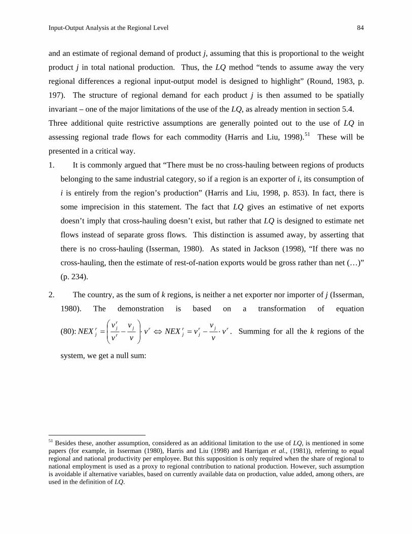
Input-Output Analysis at the Regional Level 84
and an estimate of regional demand of product j, assuming that this is proportional to the weight
product j in total national production. Thus, the LQ method “tends to assume away the very
regional differences a regional input-output model is designed to highlight” (Round, 1983, p.
197). The structure of regional demand for each product j is then assumed to be spatially
invariant – one of the major limitations of the use of the LQ, as already mention in section 5.4.
Three additional quite restrictive assumptions are generally pointed out to the use of LQ in
assessing regional trade flows for each commodity (Harris and Liu, 1998).51 These will be
presented in a critical way.
1. It is commonly argued that “There must be no cross-hauling between regions of products
belonging to the same industrial category, so if a region is an exporter of i, its consumption of
i is entirely from the region’s production” (Harris and Liu, 1998, p. 853). In fact, there is
some imprecision in this statement. The fact that LQ gives an estimative of net exports
doesn’t imply that cross-hauling doesn’t exist, but rather that LQ is designed to estimate net
flows instead of separate gross flows. This distinction is assumed away, by asserting that
there is no cross-hauling (Isserman, 1980). As stated in Jackson (1998), “If there was no
cross-hauling, then the estimate of rest-of-nation exports would be gross rather than net (…)”
(p. 234).
2. The country, as the sum of k regions, is neither a net exporter nor importer of j (Isserman,
1980). The demonstration is based on a transformation of equation
(80): rjrj
rj
rjr
rjr
j vvv
vNEXvvv
vv
NEX ⋅−=⇔⋅⎟⎟⎠
⎞⎜⎜⎝
⎛−= . Summing for all the k regions of the
system, we get a null sum:
51 Besides these, another assumption, considered as an additional limitation to the use of LQ, is mentioned in some papers (for example, in Isserman (1980), Harris and Liu (1998) and Harrigan et al., (1981)), referring to equal regional and national productivity per employee. But this supposition is only required when the share of regional to national employment is used as a proxy to regional contribution to national production. However, such assumption is avoidable if alternative variables, based on currently available data on production, value added, among others, are used in the definition of LQ.

Input-Output Analysis at the Regional Level 85
( ) ( )
01
2121
1
2211
1
=−=
+++−+++=
⎟⎟⎠
⎞⎜⎜⎝
⎛⋅−++⎟⎟
⎠
⎞⎜⎜⎝
⎛⋅−+⎟⎟
⎠
⎞⎜⎜⎝
⎛⋅−=
∑
∑
∑
=
=
=
vv
vvNEX
vv
vvvvvvNEX
vvv
vvvv
vvvv
vNEX
jj
k
r
rj
jkkjjj
k
r
rj
kjkj
jj
jj
k
r
rj
(81)
3. The region as a whole is neither a net exporter nor a net importer. In fact, if we make the
sum of the net exports for all n products of region r, we get a null sum:
01
1
11
=−=
⋅−=
∑
∑∑∑
=
=
==
rrn
j
rj
r
n
jjn
j
rj
n
j
rj
vvvvNEX
vv
vvNEX
(82)
This restriction is very limiting, since there is no theoretical reason to force the regional trade
balance with the rest of the nation to be zero.
The shortfall related to the second assumption can be prevented if the method is restricted to the
estimation of trade flows between region r and the rest of the country instead of using it to
estimate both types of trade flows (interregional and international) at the same time. In other
words, commonly accessible data on international trade should be used, in order to avoid such
restrictive assumptions as the inexistence of surplus or deficit at the nation level. However,
some adaptation must be made to the LQ method when the objective is to deal solely with
interregional trade. An appropriate variable must be used in the definition of LQ, which is
different from the effects created by international flows. Let us define the variable ,
representing available output in region r to satisfy domestic demand (demand directed to region r
and also to the remaining regions of the country) (Sargento, 2002):
rjAO
rowrj
rrowj
rj
rj dmvAO −+= , (83)
in which denotes exports of j from region r to foreign countries. Defining the LQ on the
basis of this new variable ( ), we get:
rowrjd
( ∗rjLQ )
)( ) ( )( //r r rjj j AO AOLQ AO AO
∗= (84)

Input-Output Analysis at the Regional Level 86
In this case, using an equation equivalent to (80), net exports from the rest of the country (or net
imports, if the quotient is below unity) are estimated as: the difference between the available
output in region r to satisfy domestic demand of product j and the estimated regional
requirements of product j, assuming that it is a proportion of total available output in the region
r, given by the weight of product j in domestic demand at the national level (which corresponds
to the assumption of identical regional demand structure in the region and in the country):
rjrj
rj AO
AOAO
AONEX ⋅−= (85)
If the researcher uses this version of the LQ, obtaining international trade data from an
independent source, the previously referred assumption 2 is not only appropriate, but rather a
necessary constraint. Obviously, for interregional trade flows of each commodity, it is required
that one region’s exports are equal to the imports of the rest of the regions.
In short, the LQ method suffers from the fact that it relies on two erroneous assumptions: 1) the
assumption of spatially invariant demand structure and 2) the obligation of zero balance of trade
between the region and the rest of the nation.
Commodity Balance is an alternative method to assess net commodity flows between one region
and the rest of the country. This method relies upon the balance that must hold between total
supply and total demand for each commodity. Total regional supply is equal to the sum of
regional output with regional imports; total demand is given by regional requirements plus
regional exports. Defining, as before, regional requirements of j by , the following balance
must hold, for any region:
rjD
rrocj
rrowj
rj
rocrj
rowrj
rj mmvddD ++=++ (86)
Using the previously defined variable , we obtain: rowrj
rrowj
rj
rj dmvAO −+=
rj
rj
rj
rj
rrocj
rocrj
rj
DAONEX
AOmdD
−=
=−+ (87)
When , the balance constitutes the value of net imports; when it is positive, then it
corresponds to the value of net exports.
0<rjNEX
Let us compare this equation with equation (85). Both equations attempt to estimate net exports
through the difference between available regional output and regional requirements. However,
while LQ uses a strong and unlikely assumption to provide an estimate of regional requirements

Input-Output Analysis at the Regional Level 87
for product j (given by rj AOAOAO
⋅ ), CB uses the actual value of regional requirements directly.
This suggests that, in practice, the direct use of CB should be preferred over the use of LQ. The
remark made by Stevens and Treyz (1989) provides additional support to this argument: “(…)
the alternative methods are based on the reasonable assumption that the greater the ratio of
regional supply to regional demand, the more a region is likely to buy from itself; however, LQE
and LQS measures are only proxies for this ratio, whereas the SRD is the ratio itself” (p. 252).52
But there is also a practical problem affecting CB method: it calculates as a residual,
whose value guarantees the equilibrium between supply and demand; thus, the mistakes made in
estimating the remaining components of the regional table are included in this value. Still, it has
a significant theoretical advantage over LQ since it takes into account the specific structures of
demand estimated to the region under study.
rjNEX
53 Jackson (1998) reinforces this idea stating that
“the supply-demand pool approach can be argued to be theoretically superior to methods based
on location quotients, which do not account for variations in the final demand structure” (p. 233).
This author suggests the application of CB technique in his description of how to regionalize
commodity-by-industry accounts. Commodity-balance was also applied in Jensen-Butler and
Madsen (2003) as a first step in interregional trade estimation, to obtain the net exports of each
product made by each region.
The empirical application conducted in Sargento (2002), which aimed to compare the results
provided by LQ and by CB, suggested as well that the Commodity Balance approach was the
most appropriate method to estimate trade flows between the Portuguese region under study
(Região Centro) and the rest of the country. Even with no survey data on interregional trade
flows to make an objective evaluation of each method’s accuracy, the knowledge about the
region under study allowed the author to consider that the results provided by CB were more
reasonable than the ones generated by LQ. For example, the structure of net imports suggested
by CB reflects the specific structure of intermediate consumption of the region in study which is
52 LQE and LQS stand for LQ based on employment and on supply variables, respectively; SDR is for supply-demand ratio, the author’s label for commodity-balance. 53 This is a theoretical advantage only when the technique used to estimate the vectors of regional intermediate and final demand, in assembling the regional input-output table is a suitable one. If we resort to non-survey methods applying the national structures to the region under study, without incorporating any superior information, then this advantage looses a lot of its significance. Conversely, if for example one uses surveys directed to families to estimate patterns of regional private consumption, some specific features of regional demand’s structure are being introduced, thus influencing the values of net exports estimated by CB.

Input-Output Analysis at the Regional Level 88
clearly associated with the important industries in the region. One of the paradigmatic cases
involved forestry products; the region was found to be a net exporter of these products according
to the LQ method (which may seem, at first glance, more suited to the reality of the region,
which is known by its forest extension) and a net importer, according to CB estimate. However,
taking into account the specific structure of forest products demand in the region, we realize that
intermediate demand to provide wood and cork as well as paper industries, with a great
importance in Região Centro, is by itself greater than the available regional output. Thus, the
negative sign for net trade flows given by CB method is probably a better estimate than the one
provided by LQ. Other examples concerning the empirical comparison of the results provided by
both methods can be found in Sargento (2002) and Sargento and Ramos (2003).
The option for CB technique to estimate net trade flows between one region and the rest of the
country is also patent in other empirical works carried out by Portuguese research teams, which
had the objective of assembling single-region input-output tables for other Portuguese regions.
This is the case in CCRN/MPAT (1995) applied to Região Norte and CIDER/CCRA (2001)
applied to Região do Algarve. In the construction of the input-output table for Região Autónoma
dos Açores (Azores Islands), this method was applied only partially, to services and some
residual goods, since a great part of inter-regional trade is established between the islands and the
mainland, by air and sea, for which the information provided by the Statistics of Transports and
Communications is quite complete (ISEG/CIRU, 2004).
6.3 From net to gross trade flows: the problem of crosshauling
Both methodologies presented in the previous sections lead to net trade flows (net exports, when
positive, or net imports, when negative) between the region and the rest of the country. From LQ
or CB technique, we obtain: rroc
jrocr
jrj mdNEX −= (88)
The difficulty here is that this net value may be compatible with an infinite number of values for
gross trade flows. Yet, the knowledge of the values of total gross exports and gross imports for
each region and each products is usually required to proceed with the estimation of interregional
trade flows, to complete O-D matrix for each product being traded. The problem of obtaining
gross exports and gross imports from the net trade balance is termed the crosshauling problem.
One possible option is to ignore crosshauling; in other words, when the region is a net exporter

Input-Output Analysis at the Regional Level 89
of some product, there are no imports of the same product (and, in this case, net exports will
equal gross exports). When the region is a net importer, there are no exports of the same product
(in this case, gross imports will be set equal to net imports). This is an extremely simplistic
approach, given that net flows are usually very small when compared to gross values of exports
and imports. This is demonstrated, for example, by Susiluoto (1997), in which trade between
three Finish regions was estimated both through an inquiry and using the commodity balance
method. The values of interregional trade provided by the commodity balance method were
systematically lower than the ones obtained from the inquiry, which is expected, given that the
first method accounts only for net trade flows.
Crosshauling consists in simultaneous import and export of products under the same
classification. In section 6.1 we have already addressed this issue, explaining some of the factors
that have led to an increase in crosshauling (also named intra-industry trade). What matters here
is that this is an unavoidable issue, even if a high degree of disaggregation is used in product’s
classification and in regions’ definition. It is true that, “the principle of applying a high level of
disaggregation, both in terms of commodity and geography, reduces the problem somewhat”
(Madsen and Jensen-Butler, 1999, p. 297). However, the problem would only be totally solved if
commodities were completely homogeneous or if an infinitely detailed disaggregation
concerning products and regions were used (Toyomane, 1988).
One of the possible solutions to the crosshauling problem is to set arbitrarily a crosshauling rate.
This is done for example in Madsen and Jensen-Butler (1999), in which the share is set equal to
10%. A crosshauling share χ can be defined as:
rocrj
rj
d
NEX=χ (89)
This share represents the weight of net exports (in absolute value) over gross exports. From this
crosshauling share, it is possible to achieve the value of gross exports and gross imports on the
basis of the known value of net exports. This is accomplished as follows:
⎪⎪⎩
⎪⎪⎨
⎧
+==⇒<
−==⇒>
rj
rocrj
rrocj
rjrocr
jrj
rj
rrocj
rocrj
rjrroc
jrj
NEXdmandNEX
dNEXWhen
NEXdmandNEX
dNEXWhen
χ
χ
0
0 (90)

Input-Output Analysis at the Regional Level 90
Sometimes this crosshauling share is not settled in a complete ad-hoc basis, but it is rather based
on some information on interregional trade flows available from transport statistics. This was
done, for example, in Ramos and Sargento (2003). The crosshauling shares were estimated
through the comparison between the net trade balance and total regional outflows (in physical
quantities), recorded in transport statistics. However, this is not a straightforward solution, given
the known drawbacks of transport statistics. Ramos (2001) refers five problems related to
transport statistics provided by the Portuguese national institute of statistics. First, these
statistics are only adequate to provide information on flows of goods and not on flows of
services, since interregional flows of services occur due to movements of persons and not due to
movements of products. Secondly, all trade flows are expressed in physical units, which, on the
one hand prevents the sum of flows of different products and, on the other hand, tends to
emphasize heavier products, neglecting others that may have a higher value (yet less heavy).
This last problem is reinforced by the fact that for road traffic data, all vehicles below some
weight are excluded from the population of which samples are collected. Another important
difficulty is related to the classification of goods used by transport statistics, which is not
coincident with the National Accounts classification, used in input-output table construction.
Finally, some flows recorded by transport statistics are not true interregional trade, but rather
trade between transport platforms which serve merely as points of departure (or entry) for
international exports (or imports). Thus, it is not easy to separate interregional from international
trade.
Given the difficulties in dealing with crosshauling, probably the best procedure consists in
adopting a methodology which does not require the direct estimation of crosshauling. This can
be done if the researcher opts for estimating the content of an O-D matrix comprising both intra
and interregional trade (represented in figure 7), instead of estimating the content of an O-D
interregional matrix as the one depicted in figure 6.
The elements of the matrix in figure 7 are the same as the ones in figure 6, except in what
concerns to the main diagonal and the row and column totals. The main diagonal in figure 7
comprises intra-regional trade of product j. The row sums represent total supply of product j in
region r, before accounting for interregional imports. The column sums represent total use of
product j of region s, before accounting for interregional exports. These totals correspond
exactly to the information that the researcher usually gets when the regional table is assembled,

Input-Output Analysis at the Regional Level 91
before proceeding to the estimation of interregional trade. In fact, as explained in section 6.2, net
exports are obtained by the difference between these two totals (see equation 87). It is clear that
no values of gross exports or gross imports are needed a priori (at the interregional level) to
apply such methodology; thus, the problem of crosshauling is avoided. Using this approach, the
problem of estimating interregional trade is solved in only two steps: (1) regional input-output
table assemblage, without accounting for interregional trade and (2) estimation of intra and
interregional trade flows (fulfilling the matrix of figure 7). When this matrix is fulfilled, the
researcher has access to the a posteriori values of gross imports and gross exports of product j,
for each region: they correspond to the column sums and row sums (respectively) of the off-
diagonal values of the matrix. Though, the major problem with this approach consists in finding
an adequate model to fulfill the inner part of the matrix in figure 7. Interregional trade
estimation is already a very complex problem when the objective is to estimate a matrix such as
in figure 6. When it comes to estimate a matrix like the one in figure 7 additional difficulties
arise; for example, in models that use distance between regions as one of the explaining factors
of interregional trade, one of the problems relies in finding a proper way to compute intra-
regional distance, in order to estimate the main diagonal elements of the matrix.
Figure 7: Intra and Interregional trade flows of commodity j from Region r to Region s:
. rsjx
Destination
Region 1 Region 2 … Region k Sum
Origin
Region 1 11jx 12
jx … kjx1 ( )11 row
jj mv +
Region 2 21jx 22
jx … kjx2 ( )22 row
jj mv +
… … … … …
Region k 1kjx 2k
jx … kkjx ( )krow
jkj mv +
Sum ( )rowjj dD 11 + ( )row
jj dD 22 + … ( )rowkj
kj dD +
( )( )∑
∑+
=+
s
rowsj
sj
r
rrowj
rj
dD
mv

Input-Output Analysis at the Regional Level 92
From the previous paragraph, it seems that the non-survey techniques presented on section 6.2
are options. This is true, if we are dealing with a multi-regional system of input-output tables, to
be used in multi-regional input-output analysis. In this case, the researcher can follow directly
from the table assemblage stage, where and were estimated, to the
completion of the entries in the intra and interregional trade matrices. However, if the researcher
is interested in performing input-output analysis for a single region, for instance for region 1,
then only and are achieved in the first step of assemblage. Thus, he/she will need to go
through the first two steps mentioned in section 6.1; after assembling the regional table, the net
balance of trade for each product is computed and then crosshauling must be estimated, in order
to get gross values of exports and imports.
kjj vv ,,1 k
jj DD ,,1
1jv 1
jD
Turning back to the many-region case, we still have to deal with the problem of completing the
O-D matrix (either comprised only of interregional trade or of intra and interregional trade),
using the known margin totals as restrictions of the model. This is a kind of problem which can
be approached by models belonging to the family of spatial interaction models.54
7. Conclusions. In this paper, the main objective was to provide a broad and critical review of the state of art
regarding input-output modeling and input-output table construction at the regional level. In all
sections of this paper, we were concerned with the practical applicability of the models and
techniques proposed by the literature, having in mind the quantitative and qualitative
disagreement that usually exists between the required and the available data. We tried to be
parsimonious in this theoretical review (leaving out some important topics of input-output
analysis – as for example, closing the model with respect to households, supply-side models,
dynamic models, and so on), so that it could be concise and practical oriented.
From this review, seven main conclusions may be drawn..
(1) First, it is evident that the input-output framework continues to be intensively studied
and empirically applied, in spite of its limitations, related to the set of hypotheses
underpinning the model. This means that the limitations of this framework are transcended 54 For a presentation, discussion and empirical assessment of the proposed models to solve this problem, the reader is referred to Sargento (2009).

Input-Output Analysis at the Regional Level 93
by its two main strengths: it is a fundamental tool for economic analysis (concerning the
input-output model) and it comprises a considerably detailed statistical instrument (the input-
output table).
(2) Secondly, the adaptation of the input-output framework to the regional level is extremely
important, since regional features are specific and regional problems may differ considerably
from national problems (Miller and Blair, 1985). For example, the dependence on imports
(to provide regional needs for commodity supply) and on exports (to drain regional
production) tends to be much more relevant at the smaller regional level than at the national
level (Munroe et al., 2007). For this reason, one of the most important tasks in the
construction of regional input-output tables consists precisely in the assessment of the
region’s exports and imports, which comprise trade flows established with the remaining
regions of the same country and also with other countries. In this context, the problem relies
on the estimation of interregional trade flows, since international exports and imports are
usually provided by official statistical sources.
(3) Thirdly, whenever the economic system under study includes more than one region, the
adequate input-output model to apply in this context must be capable of accounting for the
effects caused by interregional linkages – spillover and feedback effects (Miller, 1998). The
fundamental contributions of the regional field of input-output analysis, which emerged in the
1950’s, have been directed to the accomplishment of this objective, through different
versions of many-region models. These different many-region models (of which the most
important were reviewed in section 1.3) reflect different attitudes and assumptions
concerning the trade off between the degree of detail in describing interregional linkages and
the demands for trade data. In this context, the most data-demanding many-region model is
the Isard’s interregional input-output model, which is also the one that attempts to describe
interregional trade flows with the most detail. In contrast, the Chenery-Moses multi-regional
model applies certain hypotheses in order to avoid such a high demand for often unavailable
interregional trade data. More precisely, it uses the import proportionality assumption, which
states that the percentage of imports comprised in the regional demand for some specific
product is the same, regardless of the type of intermediate or final use of that product, being
given by the share of imports in the total supply of that same product. Still, a certain amount
of interregional trade data is always required to the implementation of such model: more

Input-Output Analysis at the Regional Level 94
precisely, it requires a complete origin-destination matrix for each commodity, comprised of
shipments from all possible origins to all possible destinations (without specifying the type of
user in the destination region).
(4) The database for input-output model implementation consists of the correspondent input-
output matrix (or system of matrices, in the case of many-region models). Yet, whereas at
the national level the input-output tables are regularly provided by the official statistics,
according to standardized rules, the same does not apply to the regional dimension. For that
reason, the construction of regional input-output tables continues to be, by itself, one of the
most debated themes in the regional literature. In the review of the proposed survey, non-
survey and hybrid techniques of input-output table construction, we found that, currently, it is
very difficult to find tables that are exclusively survey or non-survey (Dewhurst, 1990). In
fact, on the one hand, pure non-survey tables are criticized for being extremely mechanical,
neglecting all the specific regional features that the regional input-output table intends to
capture. Besides, there is a minimum of survey regional data (concerning, for example,
regional output and regional value added by industry) which is usually available from official
organisms of statistics, making it possible to incorporate such direct data, even for a single-
person team research, with very low budget to table construction. On the other hand, pure
survey methods involve several difficulties; the most often mentioned are its high
requirements in time, money, human and logistic resources. Other issues must be taken into
account when evaluating the possibility of survey gathering of input-output data (Jensen,
1980; Jensen, 1990). Besides some errors that may occur in the process of gathering the data,
there is a specific problem that cannot be surpassed by the allocation of more money or other
resources to the survey task: it consists simply of the fact that some questions that must be
included in the questionnaires require very detailed information to which some respondents
may not be able to answer. This problem was illustrated in the special context of the
assessment of the proportion of imported products comprised in the intermediate and final
use flows. This practical difficulty, sometimes, forces the official organisms of statistics
themselves to adopt some hypotheses, as surrogates of the information they cannot obtain
from surveys.
(5) The accuracy assessment of the constructed regional input-output table (or of any
component of it) is a quite controversial matter. First, because the benchmark for comparison

Input-Output Analysis at the Regional Level 95
(usually a survey table for the same economy) may be either not exist or it may suffer from
its own accuracy problems. Secondly, in spite of the important contribution of Jensen (1980),
the is still no general agreement on an adequate concept of accuracy in evaluating the input-
output tables. Finally, there are multiple measures of comparison between two tables, a
further subject of debate.
(6) Besides the difficulties created by non existent data (as in the case of interregional data),
another practical challenge faced by input-output researchers is qualitative mismatch between
the existing data and the model requirements. The fact is that, sometimes, input-output data
are provided in a different way from that underlying the pioneering input-output models.
Thus, input-output models must be adapted in order to fit into the specific format in which
information is available. We addressed this issue, even in a preliminary approach, focusing
on two specific topics: (i) the adaptation of the input-output model and of the techniques for
regional input-output construction to the Make and Use format and (ii) the use of techniques
to estimate intra-regional flows from total use flows (those which include imported and
regionally produced products), when no import matrices exist a priori. We were able to
exemplify, for the national and the single-region case, how the input-output model can, under
some hypotheses, be adapted to fit the Make and Use format. Concerning the second topic,
we concluded that different non-survey or partial survey techniques can be used to convert
total flows into intra-regional flows.
(7) The problem of estimating interregional trade comprises different stages, which differ
according to the number of regions under study. When dealing with single-region tables, the
first step consists in estimating net interregional trade flows. The analysis made in section
6.2 of the different techniques to achieve this goal suggests that Commodity Balance should
be preferred over Location Quotient, since: (i) it takes into account the specific structure of
demand estimated to the region under study, while LQ assumes that such structure is spatially
invariant and (ii) in contrast to LQ, it does not force the sum of interregional net exports –
that means, the regional trade balance – to be zero. After having estimated net trade flows,
crosshauling must be accounted for and gross exports and gross imports must be estimated.
Nevertheless, the estimation of crosshauling rates remains a problem to which no direct
answers exist. When we are dealing with a multi-regional system, the problem of estimating
interregional trade may be addressed in a different manner. In order to avoid the

Input-Output Analysis at the Regional Level 96
crosshauling problem, the researcher should focus on the estimation of the elements of an
intra and interregional trade matrix, for which the margin totals are known. Anyway, the
fulfillment of an O-D matrix, using the known margin totals as restrictions of the model, still
represents a problem that needs to be solved. Spatial interaction models are targeted to the
solution of this kind of problems. The study and empirical evaluation of such models is made
in Sargento (2009).
References Batten, D. 1982. "The interregional linkages between national and regional input-output models".
International Regional Science Review, 7: 53-68.
Batten, D. and Boyce, D. 1986. “Spatial interaction, transportation and interregional commodity flow
models”. In: Peter Nijkamp (ed.), Handbook of Regional and Urban Economics, 1: 357-406. Free
University, Amsterdam.
Bröcker, J. 1989. "Partial equilibrium theory of interregional trade and the gravity model", Papers of the
Regional Science Association, 66: 7-18.
Boomsma, P. and Oosterhaven, J. 1992. "A double entry method for the construction of bi-regional input-
output tables", Journal of Regional Science, 32: 269-284.
Cesario, F. and Smith, T. 1975. "Directions for future research in spatial interaction modeling", Papers of
the Regional Science Association, 35: 57-72.
CCRN/MPAT. 1995. “Quadro de Entradas e Saídas para a Região do Norte 1990: matriz de input-output”.
Ministério de Planeamento e da Administração do Território – Comissão de Coordenação da Região
Norte.
Chenery, H. 1953. “Regional Analysis”. In: Chenery, H., Clark PB (eds). The structure and growth of the
Italian economy. US Mutual Security Agency.
CIDER/CCRA. 2001. “Quadro de Entradas e Saídas para a Região do Algarve 1994: Matriz Input-Output”.
Centro de Investigação de Desenvolvimento e Economia Regional – Universidade do Algarve e Comissão
de Coordenação da Região do Algarve.
Czamanski, S. and Malizia, E. 1969. "Applicability and limitations in the use of national input-output tables
for regional studies", Papers of the Regional Science Association, 23:65-78.
de Mesnard, L. 2003. "What is the best method of matrix adjustment? A formal answer by a return to the
world of vectors". Paper presented at the 50th Annual North American Meetings of the Regional Science
Association International, Philadelphia, November 20-22nd, 2003.

Input-Output Analysis at the Regional Level 97
de Mesnard, L. 2006. “Comparing matrix adjustment methods: a formal approach”. REAL 06-T-2
(http://www2.uiuc.edu/unit/real/).
Dewhurst, J. 1990. “Using the RAS Technique as a Test of Hybrid Methods of Regional Input-Output
Table Updating”. Regional Studies, 26: 81-91.
Eding, G., Oosterhaven, J., de Vet, B., and Nijmeijer, H. 1997. “Constructing Regional Supply and Use
Tables: Dutch Experiences”. in: Hewings G, Sonis M, Madden M, Kimura Y (eds.), Understanding and
Interpreting Economic Structure. Springer Verlag, Berlin: pp. 237-63.
EUROSTAT, 1996. European System of Accounts, ESA, 1995, Luxembourg.
Fotheringham, A. and O'Kelly, M. 1989. Spatial interaction models: formulations and applications.
Dordrecht, Netherlands: Kluwer Academic Publishers.
Glasmeier, A. 2004. "Geographic intersections of regional science: reflections on Walter Isard's
contributions to geography". Journal of Geographical Systems, 6: 27-41.
Goldman, M. 1969. "Comments on Czamanski and Malizia". Papers of the Regional Science Association,
23: 79-80.
Greytak, D. 1969. "A statistical analysis of regional export estimation techniques", Journal of Regional
Science, 9: 387-397.
Greytak, D. 1970. "Regional impact of interregional trade in input-output analysis", Papers of the Regional
Science Association, 25: 203-217.
Harrigan, F. 1990. "The reconciliation of inconsistent economic data: the information gain", Economic
System Research, 2(1): 17-25.
Harrigan, F., McGilvray, J.W. and I. H. McNicoll. 1980. “A comparison of regional and national technical
structures”. The Economic Journal, 90: 795-810.
Harrigan, F., McGilvray, J.W. and I. H. McNicoll. 1981. "The estimation of interregional trade flows",
Journal of Regional Science, 21(1): 65-78.
Harris, R., Liu, A. 1998. "Input-output modeling of the urban and regional economy: the importance of
external trade", Regional Studies, 32.9: 851-862.
Hewings, G. 1983. "Design of appropriate accounting systems for regional development in developing
countries" Papers of the Regional Science Association, 51: 179-195.
Hewings, G. and Jensen, R. 1986. “Regional, Interregional and Multiregional Analysis”. In: Peter Nijkamp
(ed.), Handbook of Regional and Urban Economics, 1: 295-355. Free University, Amsterdam.
Hewings, G., Sonis, M., Guo, J., Israilevich, P and Schindler, G. (1998) “The hollowing out process in the
Chicago economy, 1975-2015,” Geographical Analysis, 30: 217-233.
Isard, W. 1951. "Interregional and regional input-output analysis: a model of a space-economy", Review of
Economic and Statistics, November, pp. 318-329

Input-Output Analysis at the Regional Level 98
ISEG/CIRU – Instituto Superior de Tecnologia e Gestão / Centro de Investigações Regionais e Urbanas.
2004. "Sistema de Matrizes Regionais de Input-output para a Região Autónoma dos Açores - Relatório
metodológico e resultados". Ed.: Subsecretário Regional do Planeamento e Assuntos Europeus, Direcção
Regional de Estudos e Planeamento.
Isard, W. 1975. "A simple rationale for gravity type behavior", Papers of the Regional Science Association,
35: 25-30.
Isard, W. 1998. “Gravity and spatial interaction models”. In: Walter Isard et al., Methods of interregional
and regional analysis, pp. 243-280. Ashgate Publishing Limited.
Isard, W. and Bramhall, D. 1960. "Gravity, potential and spatial interaction models". In: W. Isard, Methods
of regional analysis, pp. 493-568. Cambridge, Mass: MIT Press.
Israilevich, P., Hewings, G., Schindler, G. and Mahidhara, R. 1996. “The choice of an input-output table
embedded in regional econometric input-output models”. Papers in Regional Science, 75(2): 103-119.
Isserman, A. 1980. “Estimating Export Activity in a Regional Economy: A Theoretical and Empirical
Analysis of Alternative Methods” International Regional Science Review, 5(2): 155-84.
Jackson, R. 1998. "Regionalizing national commodity-by-industry accounts", Economic Systems Research,
10(3): 223-238.
Jackson, R. and Murray, A. 2004. "Alternate Input-output matrix updating formulations". Economic
Systems Research, 16(2): 135-148.
Jackson, R., Schwarm, W., Okuyama, Y., Islam, S. 2006. “A method for constructing commodity by
industry flows”, Annals of Regional Science, 40(4): 909-920.
Jackson, D. 2000. The new National Accounts: an introduction to the System of National Accounts 1993
and the European System of Accounts 1995. Ed.: Edward Elgar, Northampton, MA, USA.
Jensen, R. 1980. “The concept of accuracy in regional input-output models”. International Regional
Science Review, 5: 139-154.
Jensen, R. 1990. “Construction and use of regional input-output models: progress and prospects”,
International Regional Science Review, 13(1&2): 9-25.
Jensen-Butler, C. and Madsen, B. 2003. “Intraregional and interregional trade in regional commodity
balances: estimation and results for Denmark”, Paper presented at the 50th Annual North American
Meeting of the Regional Science Association International, Philadelphia 20-22 November, 2003.
Koutaniemi, M. and Louhela, T. 2006. “Construction of Regional Input-Output Tables in Finland 2002”.
Paper presented at the 46th Congress of the European Regional Science Association, University of
Thessaly, Greece, August 30th-September, 3rd, 2006.
Lahr, M. 1993. “A review of the literature supporting the hybrid approach to constructing regional input-
output models”. Economic Systems Research, 5: 277-293.

Input-Output Analysis at the Regional Level 99
Lahr, M. 1998. “A strategy for producing hybrid regional input-output tables”. Paper presented at the 12th
International Conference on Input-output Techniques, New York City, May 21, 1998.
Lahr, M. 2001. "Reconciling domestication techniques, the notion of re-exports, and some comments on
regional accounting". Economic Systems Research, 13(2): 165-179.
Lahr, M. and de Mesnard, L. 2004. “Biproportional techniques in input-output analysis: table updating and
structural analysis”, Economic Systems Research, 16(2): 115-134.
Leontief, W. 1953. “Interregional Theory”. In: Leontief, WW, Chenery HB, Clark PG. Studies in the
structure of the American economy. Oxford University Press, New York, pp. 93-115.
Madsen, B. and Jensen-Butler, C. 1999. “Make and Use approaches to regional and interregional accounts
and models”. Economics Systems Research, 11(3): 277-299.
Martinez-Zarzoso, I. 2003. “Gravity model: an application to trade between regional blocks”, Atlantic
Economic Journal, 31: 174-187.
Martins, J., Castro, E., Ramos, P., Abreu, D., Borrego, C., Marques, J., Lopes, M., Fernandes, M., Mendes,
D., Couto, J., Santos, R., Soares, A., Sargento, A. 2005. “OIKOMATRIX II: Avaliação do impacto sócio-
económico a nível regional de instrumentos legais de controlo das emissões de gases com efeito estufa”.
Fundação para a Ciência e Tecnologia, POCTI/MGS/41874/2001.
Miller, R. 1998. “Regional and Interregional Input-Output Analysis”. In: Walter Isard et al., Methods of
interregional and regional analysis, pp. 41-134. Ashgate Publishing Limited.
Miller, R. and Blair, P. 1985. Input-Output Analysis – Foundations and Extensions. Prentice-Hall (ed.).
Miller, R. 1966. “Interregional feedback effects in input-output models: some preliminary results”, Papers
of the Regional Science Association, 27: 105-125.
Mohr, M., Crown, W.H. and Polenske, K.R. 1987. "A linear programming approach to solving infeasible
RAS problems", Journal of Regional Science, 27(4): 587-603.
Morrison, W. and Smith, P. 1974. “Nonsurvey input-output techniques at the small area level”, Journal of
Regional Science, 14 (1): 1-14.
Moses, L. 1955. “The stability of interregional trading patterns and input-output analysis”. American
Economic Review, 45: 803-832.
Munroe, D. Hewings, G. and Guo, D. 2007. “The Role of Intraindustry Trade in Interregional Trade in the
Midwest of the US” In R. Cooper, K. Donaghy and G. Hewings . (eds.), Globalization and Regional
Economic Modeling, Heidelberg, Springer-Verlag.
Nijkamp, P. and Paelinck, J. 1974. “A dual interpretation and generalization of entropy-maximization
models in regional science”. Papers of the Regional Science Association, 33:13-31.
O'Kelly, M. 2004. “Isard's contributions to spatial interaction modeling”. Journal of Geographical Systems,
6: 43-54.

Input-Output Analysis at the Regional Level 100
Oosterhaven, J. 1984. “A family of square and rectangular inter-regional input-output tables and models”.
Regional Science and Urban Economics, 14: 565-582.
Oosterhaven, J., Piek, G. and Stelder, D. 1986. “Theory and practice of updating regional versus
interregional interindustry tables”. Papers of the Regional Science Association, 59: 57-72.
Oosterhaven, J. and Stelder, D. 2007. “Evaluation of non-survey international input-output construction
methods with the Asian-Pacific input-output table”. Papers and Proceedings of the International
Workshop Emergence of Chinese Economy and Re-organization of Asian Industrial Structure, December
14-15, 2006.
Park, S., Mohtadi, M. and Kubursi, A. 1981. “Errors in Regional nonsurvey input-output models: analytical
and simulation results”. Journal of Regional Science, 21: 321-337.
Piani, G. and Kume, H. 2000. “Fluxos bilaterais de comércio e blocos regionais: uma aplicação do modelo
gravitacional”, Texto para discussão nº749, Instituto de Pesquisa Economia Aplicada.
Piispala, J. 1998. “Regional Input-output tables based on supply and use framework: the Finnish case”.
Paper presented at the Structures and Projects of Nordic Regional Economics, 4-7 June, 1998.
Piispala, J. 2000. “On regionalising Input-output tables - Experiences from compiling regional supply and
use tables in Finland”. Paper presented at the XIII International Conference on Input-output Techniques at
University of Macerata, Italy, August 21-25th, 2000.
Polenske, K. 1970a. “Empirical implementation of a multiregional input-output gravity trade model”. In: A.
P. Carter and A. Brody, eds., Contributions to input-output analysis. Amsterdam: North-Holland, 143-
163.
Polenske, K. 1970b. “An empirical test of interregional input-output models: Estimate of 1963 Japanese
production”. American Economic Review, 60:76-82.
Polenske, K. 1995. “Leontief's spatial economic analyses”, Structural Change and Economic Dynamics, 6:
309-318.
Polenske, K. and Hewings, G. 2004. “Trade and spatial economic interdependence”, Papers in Regional
Science, 83: 269-289.
Porojan, A. 2001. “Trade flows and spatial effects: the gravity model revisited”, Open Economies Review,
12(3): 265-280.
Ramos, P. 2001. “Comércio intra e inter-regional no Continente Português: a perspectiva das estatísticas
dos transportes”. Cadernos Regionais, Região Centro, nº12.
Ramos, P. and Sargento, A. 2003. “Estimating trade flows between Portuguese regions using an input-
output approach”. Paper presented at the 43rd Congress of the European Regional Science Association,
Jyväskylä (Finland), August 27-30, 2003.

Input-Output Analysis at the Regional Level 101
Riefler, R. and Tiebout, C. 1970. “Interregional input-output: an empirical California-Washington model”.
Journal of Regional Science, 10: 135-152.
Robinson , D. and Liu, Z. 2006. “The effects of interregional trade flow estimation procedures on
multiregional social accounting matrix multipliers”. The Journal of Regional Analysis and Policy, 36(1):
94-114.
Round, J. 1978a. “On estimating trade flows in interregional input-output models”, Regional Science and
Urban Economics, 8:289-302.
Round, J. 1978b. “An interregional input-output approach to the evaluation of nonsurvey methods”. Journal
of Regional Science, 18:179-194.
Round, J. 1983. “Non-survey techniques: a critical review of the theory and the evidence”. International
Regional Science Review, 8: 189-212.
Roy, J. and Thill, J. 2004. “Spatial interaction modeling”, Papers in Regional Science, 83: 339-362.
Sargento, A. 2002. “Matriz de Input-Output e estimação do comércio inter-regional – um estudo para a
Região Centro” Dissertation for obtaining the master degree on Economics - Faculdade de Economia da
Universidade de Coimbra.
Sargento, A. 2006. “Empirical Examination of the Gravity Model in Two Different Contexts: Estimation
and Explanation”. Paper presented at the International Conference on Regional and Urban Modeling,
Brussels, June 1-2, 2006.
Sargento, A. e Ramos, P. 2003. “Matriz Input-Output e Comércio Inter-regional na Região Centro
(Portugal)”. Revista Portuguesa de Estudos Regionais, nº3, pp.5-23, Lisboa, Instituto Nacional de
Estatística e APDR.
Sargento, A. 2009. “Regional input-output tables and models: interregional trade estimation and input-
output modeling based on total use rectangular tables”, PhD Dissertation in Economics, Faculty of
Economics – University of Coimbra.
Schaffer, W. and Chu, K. 1969. “Non-survey techniques for constructing regional interindustry models”,
Papers and Proceedings of the Regional Science Association, 23: 83-101.
Sen, A. and Smith, T. 1995. Gravity models of spatial interaction behavior, Springer-Verlag, Berlin.
Soloaga, I. and Winters, A. 1999. “Regionalism in the nineties: what effects on trade?”, Development
Economic Group of the World Bank.
Snickars, F., Weibull, J. 1977. “A minimum information principle”, Regional Science and Urban
Economics, 7: 137-168.
Stevens, B. and Treyz, G. 1989. "On the comparative accuracy of RPC estimating techniques". In:
Frontiers of Input-output Analysis, Ronald E. Miller, Karen R. Polenske and Adam Z. Rose (eds), New
York, Oxford University Press.

Input-Output Analysis at the Regional Level 102
Susiluoto, I. 1997. "Regional economic growth: an input-output study of the Helsinki region". Paper
presented at the 37th Congress of the European Regional Science Association, Rome, Italy, 26-29 August
1997.
Theil, H. 1967. Economics and information theory, Amsterdam: North-Holland.
Toyomane, N. 1988. Multiregional Input-output models in long-run simulation. Kluwer Academic
Publishers, Dordrecht.
UN – United Nations, 1993. System of National Accounts 1993 – SNA 1993. United Nations Statistical
Division – National Accounts. New York.
Van Der Linden, J. and Oosterhaven, J. 1995. "European Community intercountry input-output relations:
construction method and main results for 1965-85". Economic Systems Research, 7(3):249-270.
West, G. 1990. "Regional Trade Estimation: A Hybrid Approach", International Regional Science Review,
13(1&2): 103-118.
Willekens, F. 1983. “Log-Linear modeling of spatial interaction”, Papers of the Regional Science
Association, 52: 187-205.
Wixted, B., Yamano, N. and Webb, C. 2006. "Input-output analysis in an increasingly globalised World:
applications of OECD's harmonised international tables". STI Working Paper 2006/7, OECD, Paris.