1

CHAPTER 1

INTRODUCTION

1.1 GENERAL

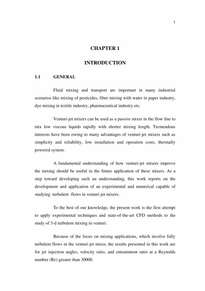
Fluid mixing and transport are important in many industrial

scenarios like mixing of pesticides, fibre mixing with water in paper industry,

dye mixing in textile industry, pharmaceutical industry etc.

Venturi-jet mixers can be used as a passive mixer in the flow line to

mix low viscous liquids rapidly with shorter mixing length. Tremendous

interests have been owing to many advantages of venturi-jet mixers such as

simplicity and reliability, low installation and operation costs, thermally

powered system.

A fundamental understanding of how venturi-jet mixers improve

the mixing should be useful in the future application of these mixers. As a

step toward developing such an understanding, this work reports on the

development and application of an experimental and numerical capable of

studying turbulent flows in venturi-jet mixers.

To the best of our knowledge, the present work is the first attempt

to apply experimental techniques and state-of-the-art CFD methods to the

study of 3-d turbulent mixing in venturi.

Because of the focus on mixing applications, which involve fully

turbulent flows in the venturi-jet mixer, the results presented in this work are

for jet injection angles, velocity ratio, and entrainment ratio at a Reynolds

number (Re) greater than 30000.

2

1.2 MOTIVATION

In order for the applications of transverse turbulent jet mixing of

two fluids at required proportion with shorter mixing length for industrial

applications, a method of jet mixing with crossflow must be developed. In

certain mixing applications, this is done by attaching a device called venturi-

jet mixer in the crossflow pipe line.

In addition to proportional mixing, attributes of the device include

elimination of additional pump and mixing enhancement. The mixer uses the

momentum of the crossflow to create a suction effect to pump in a secondary

flow (jet) of high tracer concentration. The jet and cross flows are then mixed

over a surface of complex geometry, transferring momentum to the jet.

The device also affects the pressure at the exit of the mixer, thus

affecting the power requirement of the mixer. Conventional transverse jet

mixers operate at low Reynolds number and require a secondary pump to

inject the jet into the crossflow. The venturi-jet mixer would operate at high

Reynolds number to produce the suction effect and the required mixing

quality by turbulence.

Very little work on venturi-jet mixers has been published.

However, some of the work (Boume and Garcias-Rosas 1986, Studer 1990)

reports that they show promise as passive mixers because of the extremely

intense turbulence that they produce without mixing elements.

The effectiveness of a venturi-jet mixer depends upon many things,

for example the flow pattern, pressure drop and rate of mixing; when

designing the mixer it is advantageous to have knowledge of these quantities.

It is also desirable to have other information, such as concentration decay, jet

3

path, jet velocity decay and how the mixer will contribute to pumping the

process fluid. All of this information is sparse in the literature.

Since the availability of information required to design the mixer is

limited, this work aims to improve the state of the knowledge - through an

experimental and numerical study. Flow rates of the flowing fluids,

concentration distribution information and pressure drop data need to be

produced to allow the design of a venturi-jet mixer. Therefore the research

was specifically focussed on the investigation of in-line mixer that fits into a

process pipeline.

1.3 NEED FOR THE RESEARCH

The conventional mixing of the primary and secondary flow in a

mixing tube is very slow, which is performed mainly by a small scale viscous

mixing in a shear layer. Thus, a conventional mixer requires a long mixing

tube to entrain the secondary flow. Also a long mixing tube results in large

wall friction loss, extra weight and higher cost. Their performance is

unsatisfactory or unreliable when ratio adjustments are required.

On account of the above disadvantages of conventional systems,

venturi-jet mixer systems have received great attention by many researchers

in the recent years and they have been widely applied to the fluid mixing area.

A venturi-jet mixer is a simple device for mixing two fluid streams.

Researchers have reported jet trajectories, mixing pattern, pressure drop data,

and G-value for variety of static mixers except venturi-jet mixers over the past

few decades.

Passive mechanisms have been studied extensively, however,

previous research on passive mixing by venturi-jet mixer has concentrated on

4

typically one of the geometric factors, and an overall view of geometric

configuration and their effect on mixing is not clear.

None of the previous studies considered the effects of increased

flow rate, inertia and varied injection angle. With the transverse jet mixing,

the flow distance required to achieve a certain degree of mixing is a function

of both the method of injection and the crossflow mixing governed by

crossflow characteristics (Fitzgerald and Holley 1979).

In order to improve the efficiency of such devices, it is important to

obtain more insight into turbulent mixing. In the numerical and experimental

investigation of turbulent mixing, it is necessary to obtain the velocity and

concentration field, simultaneously, since the mixing process can be described

as the interaction between a velocity and concentration field.

Jet injection systems due to suction effect created by the crossflow

in the venturi-jet mixer were the subject of this investigation because the

mixing is greatly enhanced by the turbulence and counter rotating vortex pair

created just downstream of injection. In brief, passive mixing by using

venturi-jet mixer is challenging and attracts the attention of many researchers.

This work presents the results for a wide range of jet injection

angles and Reynolds number in a venturi-jet mixer. In this thesis, mixing of

two streams with similar physical properties and different tracer concentration

is focussed. The jet trajectories and mixing performance is determined by

numerical procedure and experimental data.

Because of the focus on the mixing applications, which involve

fully turbulent flows, the results presented in this work are different injection

angles (45o

o 135o) and jet to cross flow momentum ratio for a span of

Reynolds number based on hydraulic diameter from 32000 to 51000.

5

In the present work, five arbitrary injection angles 45o, 60

o, 90

o,

120o and 135

o are studied numerically and experimentally to investigate the

effect of injection angle on the mixing performances of venturi-jet mixer

systems. In this study the cross flow effect on the jet motion, such as on jet

trajectory, jet width growth, and concentration decay in venturi-jet mixer is

predicted by mathematical calculation.

An experimental investigation is used to validate the conservation

equations derived theoretically based on the mass, momentum and tracer

concentration written in natural coordinate system and to compare the results

obtained using CFD analysis. The effect of the jet angle and momentum ratio

on the trajectory and mixing has also been studied experimentally and

numerically as it is significant in obtaining an optimum engineering design.

1.4 OBJECTIVES AND SCOPE OF THE RESEARCH

The primary objective of this work is to characterize the

performance of venturi-jet mixers at high Reynolds numbers and at different

jet injection angles. Tests were conducted on the venturi-jet mixers of varied

jet injection angles at high Reynolds numbers.

Concentration, flow rates, and pressure obtained from those tests

are used to determine the performance of the mixers in terms of concentration

decay, jet to crossflow pumping and mixing metrics.

The experimental results are then compared to the numerical

solutions obtained from mathematical formulations in natural coordinate

system and CFD analysis. The end result serves as a base of knowledge useful

to the design of a venturi-jet mixer. To accomplish the primary objective, two

major objectives and sub objectives are evolved and performed.

6

The major objectives of this work as follows:

The first major objective is to experimentally and theoretically

analyse by writing the conservation equations in natural

coordinate system to explore the effects of concentration

dependent fluid properties on the flow structure and mixing

characteristics of transverse jet in a venturi-jet mixer (novel in-

line mixer) without mechanical assists.

To set up a suitably instrumented flow loop system

incorporating the venturi-jet mixer unit.

Mathematical formulation of the mixer in natural coordinate

system along with the initial and boundary conditions.

Obtaining solutions for the partial differential equations by

finite difference method.

Comparing the numerical results for jet trajectories and

mixing behaviour of the mixer with the experimental results.

Arriving at the correlations for jet trajectories and

concentration decay by multi-variate regression analysis.

Calculation of velocity ratio and entrainment ratio and

plotting them with respect to jet injection angles and

crossflow Reynolds number.

Studying the influence of jet injection angles and crossflow

Reynolds number on jet trajectories and mixing performance

of the mixer.

7

The second major objective is to analyse the mixer

characteristics using CFD package.

Choosing the appropriate turbulence model for the study.

Modelling and meshing the mixer using GAMBIT software.

Fixing the mesh size of the mixer by comparing the

turbulent kinetic energy.

Solving the model by applying the boundary conditions

using FLUENT software.

Presenting the plane concentration profile of the jet in the

downstream locations.

Comparing the predicted jet trajectories and mixing

performance with the experimental results.

The scope of this research is restricted by several aspects. High

Reynolds number turbulence flow happens to be prevailing for low viscous

mixing fluids in the venturi-jet mixer. For the jet diameter of 1 or 2mm, the

mass of entraining fluid is very much less compared to mass of motive fluid.

Hence the entrainment ratio is low.

Many industrial mixing processes take place in two phases, under

turbulent flow conditions, because the mixing properties of turbulent flows

are superior to the ones of laminar flows (Ottino 1990). Therefore, highly

viscous fluids with large entrainment ratio and two phase mixing are outside

of the scope of this research. The research focuses on turbulent mixing of two

liquids with nearly water density and less entrainment ratio in the mixer.

8

The outcome of this study could be useful to further understand the

flow and mixing characteristics in the venturi-jet mixer at various jet injection

angles and operating conditions and to design such a mixer.

1.5 LITERATURE REVIEW

A review of the literature on the jets in crossflow, scalar variance,

CFD, as well as previous research of venturi-jet mixer systems is provided in

this chapter.

A literature review was performed on the jets in crossflow since it

was used to obtain the flow and mixing behaviour of fluids in order to

validate the numerical model with the experimental data.

As mixing in venturi-jet mixer comprised by turbulent jet in the

venturi, previous works of jet in crossflow were also looked at so that basic

insight into such structures can be gained in order to obtain jet trajectories

correlation.

Similarly, scalar variance was studied, as concentration decay

correlations along the mixer downstream distances, shall be developed from

the numerical models made.

Finally, in this section some basics of CFD and earlier work done

in the CFD analysis of the transverse jet mixers were discussed as it provides

insight on the modelling procedures and techniques used to obtain accurate

results of the mixer.

1.5.1 Jet in Crossflow

Jet in crossflow (JICF) configuration is typically constituted by a

jet that issue into a cross-flow. Turbulent jets in a crossflow have been used in

9

many engineering fields. Among various configurations of jets in a crossflow,

turbulent plane jets injected normally into a uniform cross stream have

numerous applications. Industrial mixing, film cooling, effluent discharged

into the atmosphere and into water bodies are a few examples of such

applications.

1.5.2 Physical Flow Phenomenon of JICF

The complicate nature of the JICF is illustrated in Figure 1.1, where

the flow behaviour for a velocity ratio R = 2 is represented. This figure was

obtained from the flow-visualization measurements of Foss (1980), and from

the velocity measurements of Andreopoulos and Rodi (1984).

Figure 1.1 Schematic diagram of the vortex system associated with

the JICF

The most obvious feature of the JICF is the mutual deflection of jet

and crossflow. The jet is bent over by the cross-stream, while the cross-stream

is deflected as if it were blocked by a rigid obstacle. Figure 1.1 shows also

that the fundamental characteristics of the JICF are dominated by a complex,

three-dimensional, inter-related set of vortex systems in the lee of the jet.

10

1.5.3 Class Structures of Vortices

With reference to Figure 1.1, Vanessa et al. (2005) classified the

main structures as follows:

Class 1 structures

Class 2 structures

1.5.3.1 Class 1 structures

The class 1 structures are originated by the interaction of the jet

with the crossflow and the wall and cannot be recognized in free jets (Vanessa

et al. 2005). Among structures of this kind the following vortex systems are

included (Andreopoulos 1984 and Camussi 2002):

Counter-Rotating Vortex Pair (CRVP)

Horseshoe Vortices (HSV)

Upright vortices (UV)

Counter-rotating vortex pair (CRVP)

The CRVP, Figure 1.2, is the most dominant vortex system and is

generated as an effect of the bending of the jet itself. The mechanism for the

formation of the CRVP is not yet fully understood. It can be taken as certain,

that the vorticity of the CRVP has its origin at the side-walls of the jet.

In fact, Haven et al. (1997) investigated different nozzle geometry

for the jet and discovered that for rectangular jets the amplitude of the CRVP

depends on the aspect ratio of the jet section. A variety of interpretations of

CRVP and its origin have evolved over the years. In general, however, CRVP

is widely viewed to be formed by the vortex sheet or thin shear layer

emanating from the jet nozzle.

11

Figure 1.2 Counter-rotating vortex pair

It is generally accepted that the shear layer of the jet folds and rolls

up very near to the pipe exit, leading to or contributing to the formation of the

CRVP, although there are questions pertaining to the nature of vortex roll-up

near the jet exit. Tilting and folding of the vortical structures are seen to

contribute to the downstream components of vorticity which form, on an

averaged basis, counter-rotating vortical structures. The origin and

development of the CRVP are important because control of vorticity

generation and evolution is a mean of controlling transverse jet mixing and,

potentially, reaction processes.

Horseshoe vortices (HSV)

The HSV, Figure 1.3, is formed upstream of the jet and close to the

wall and result from the interaction between the wall boundary layer and the

round transverse jet. HSV are found to be steady, oscillating, or coalescing.

Frequencies of oscillation have been found to be correlated with periodic

motions of upright vortices.

Upright vortices (UV)

The UV are generated by the interaction of the wall boundary layer

with the jet flow and, for low Rej , are the only unsteady structure.

12

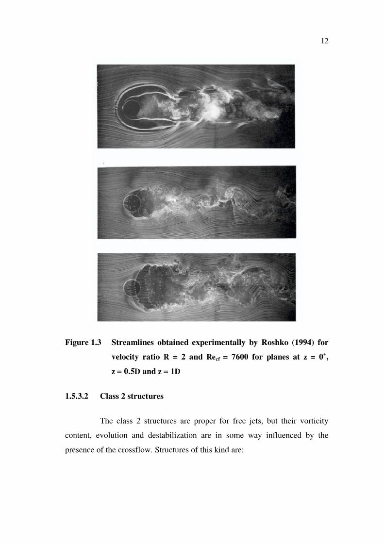
Figure 1.3 Streamlines obtained experimentally by Roshko (1994) for

velocity ratio R = 2 and Recf = 7600 for planes at z = 0+,

z = 0.5D and z = 1D

1.5.3.2 Class 2 structures

The class 2 structures are proper for free jets, but their vorticity

content, evolution and destabilization are in some way influenced by the

presence of the crossflow. Structures of this kind are:

13

Ring-Like Vortices (RLV)

The Ring-Like Vortices (RLV) are formed from the shear layer of

the jet flow and their shape and spatial evolution is distorted by the presence

of the cross-stream. With the CRVP, they determine the dominant features of

the velocity and vorticity fields and their dynamics is of great interest from

the practical viewpoint since they are mainly responsible for mixing and for

mass, momentum and heat transfer.

1.5.4 Three Distinct Regions of JICF

Krothapalli et al. (1981), Raman and Taghavi (1996), and Smith

and Mungal (1998), divided the flow obtained from a JICF into three regions;

the potential core region, in the first few diameters from the jet exit; the near-

field region, just beyond the potential core, where the flow is fully turbulent

but has not deflected appreciably, and the far-field region, where the jet’s

flow has turned almost completely into the crossflow.

Demuren (1986), Sherif and Pletcher (1991), Said et al. (2005) also

classified the jet flow field of jet in crossflowing stream into three distinct

regions. In the first region, the initially uniform jet flow interacts with the

ambient crossflow causing a shear layer to develop at the jet boundaries.

Upstream of this region, the crossflow is decelerated and a positive pressure

region is formed. The length of the initial region depends on the jet diameter,

velocity ratio and jet discharge Reynolds number.

The second region is the main region or the established flow region,

where the jet experiences maximum deflection. This region is complex, being

characterized by the development of turbulent mixing layer around the jet

boundaries and the flow becomes fully turbulent. Due to shearing action of

the crossflow, the jet sides experience strong lateral deflections.

14

The third region is the far field region, where the jet axis

approaches the crossflow direction asymptotically and the flow field becomes

nearly self-similar. In this region, the magnitude and direction of the jet

velocity are close to those of the cross flowing stream and it becomes difficult

to distinguish between crossflow and jet fluids.

1.5.5 Early Jet Mixing Researches

Investigations on the JICF have started in the 1930s (Schlichting

and Andew 1933). Since, there have been numerous investigations on the

JICF leading to the perception that the JICF, in contrast to other flows like

jets and mixing layers, cannot be described in terms of self similarity and

Reynolds dependence, due to the strong nonlinear effects. The systematic

analysis of the JICF started in 1970s with the discovery and acceptance of

coherent structures that are able to explain various nonlinear effects in the

JICF. Figure 1.1 shows JICF with associated counter rotating pair of vortical

structure.

Carter (1969) studied heated turbulent plane jets in a confined

crossflow where he measured the temperature trajectories, defined as the

locus of local maximum temperature, for three different values of jet to cross

stream velocity ratios (R).

Kamotani and Greber (1972) measured the velocity and

temperature distribution downstream of a heated turbulent round jet injected

into a subsonic cross-flow for several momentum-flux ratios. The results

showed that the jet structure is primarily dominated by a vortex pair formed

behind the jet. At lower flux ratios, the jet is deflected sharply and the vortices

do not have time to develop. Therefore, the kidney shape structure remains

present into the far downstream. However at higher momentum flux ratios the

vortices become stronger and dominate the flow field. The results also

15

indicated that the jet velocity and temperature trajectories strongly depend

upon the momentum flux ratio.

Turbulent jets in crossflows have been investigated extensively

(Rajaratnam 1976 and Wright 1977). Wright (1977) divided the flow in the

deflected jet into two main regions, referred to as the momentum dominated

near field (MDNF) and the momentum dominated far field (MDFF). The

MDFF is followed by a passive plume region (PPR) where the mixing and the

resulting dilution are due to the turbulence in the ambient flow. The transition

from the MDFF to the PPR was assumed (Rajaratnam and Langat 1995) to

occur where the excess velocity in the jet above that of the crossflow velocity,

v falls to about 1% of (uo-v) where uo is the velocity of the jet at the nozzle.

Maruyama et al. (1981, 1982) studied the jet injection of fluid into

the pipeline over several pipe diameters from the injection point, and

proposed the standard deviation as an indication of mixing quality.

The dilution characteristics and the plume trajectory of the tee

diffusers have been studied by several investigators in order to provide basic

information for the siting and design of the diffuser (Adams 1982).

Andreopoulos and Rodi (1984) reported on measurement in flow

generated by a jet issuing from the circular outlet in a wall into a cross-stream

along this wall. A quantitative picture of complex three-dimensional mean

low and turbulence field and the velocity ratio dependence parameters were

presented.

Ferrell and Lilley (1985) conducted experiments of the flow field of

a deflected jet in a confined (non-swirling) cylindrical crossflow. They found

that the jet penetration was reduced from that of comparable velocity ratio

infinite crossflow cases. Their measurements confirmed that the deflected jet

is symmetrical about the vertical plane passing through the cross-flow axis.

16

Isaac and Jakubowski in 1985 performed detailed velocity and

Reynolds stress measurements of twin jets injected normally to a crossflow.

Their results showed a striking similarity in terms of mean velocities and

turbulent parameters between the tandem jets and a single jet in a crossflow

(Hatch et al. 1996).

A jet exhausting perpendicularly into a crossflow deflects,

increases in lateral extent, distorts in cross sectional shape and evolves into a

flow field that is dominated by a pair of counter-rotating vortex (CVP) (Roth

1988).

Vranos et al. (1991) conducted an experimental study of jet mixing

in a cylindrical duct. Planar digital imaging was used to measure the

concentration of an aerosol seed uniformly mixed with the jet stream, in

several planes downstream of the mixing orifices. The results showed that for

an axis-symmetric geometry, mixedness was more sensitive to circumferential

uniformity rather than jet penetration.

1.5.6 Recent Jet Mixing Researches

Many attempts have been made by the researchers over the past

decade to analyse the flow phenomenon and also to improve the mixing

efficiency of a jet in crossflow.

A heated and unheated lateral jets discharging into a confined

swirling cross flow was numerically investigated by Chao and Ho (1992).

They studied variations of parameters like jet temperature, jet-to-crossflow

velocity ratio, jet number and swirl length. The results show that the jet

decaying process is almost independent of the temperature difference between

the heated jet and the crossflow. The jet spreading process is dependent on the

inlet mass flux ratio and the mixing conditions.

17

Margason (1993) provided an extensive review of past work before

1993 on jet in cross flow. In many of the studies, the main interests are the

trajectories prediction, the formation, evolution and interaction of CRVP and

their respective applications. Both experimental and computational efforts

were conducted to investigate the details of different flow structures of JICF.

Sarkar and Bose (1995), predicted characteristics of a two-

dimensional turbulent plane jet in a crossflow where a cold jet stream is

discharged into a strong cross stream ( 1.0). They computed flow field and

surface temperature distributions along with the turbulence quantities to

illustrate the flow physics involved.

Su and Mungal (1999) conducted experiments to analyse the

structure and scaling of the velocity and scalar fields using PIV and PLIF

measurement techniques. The measurements provided a comprehensive view

of the velocity and conserved scalar fields in the developing region of the flow.

All measurements are made at a single jet-to-crossflow velocity ratio of 5.7.

A round jet injected into a confined cross flow in a rectangular

tunnel was simulated using Reynolds-averaged Navier-Stokes equation with

the standard k- turbulence model by Holdeman et al. (1999). The principal

observations was that the turbulence Schmidt number had a significant effect

on the prediction of the species spreading rate in jet in crossflow, especially

for the cases where the jet-to-crossflow momentum flux are relatively small.

Kalyan et al. (2002) performed numerical predictions of turbulent

plane jets discharged normal to a weak or moderate cross stream. The

Reynolds-averaged Navier–Stokes equations with the standard k- turbulence

model have been used to formulate the flow problem. The results show that

while mixing of the two streams the local maximum mean velocity (um)

decreases along the jet trajectory. Also, it was concluded that the amount of

18

penetration of the jet into the crossflow and deflection of the jet depend upon

the value of velocity ratio.

Wegner et al. (2004) studied turbulent mixing using Large Eddy

Simulation (LES). They varied the angle between the jet and the crossflow.

The mixing was enhanced as the angle was increased i.e. as the jet was

directed against the crossflow. The baseline flow in their simulation was that

measured by Andreopoulos and Rodi (1984).

Petri and Timo (2006) performed the Large Eddy Simulation (LES)

of a turbulent jet in a cross-flow with steady-state and unsteady boundary

conditions. On the whole differences between the cases are relatively small in

this flow. The LES with the unsteady condition possesses a stronger back-

flow in the lee of the jet where the cross-stream-wise velocity profiles along

the vertical lines are steeper.

Manabendra et al. (2006) performed a computational investigation

of three-dimensional mean flow field resulting due to the interaction of a

rectangular heated jet issuing into a narrow channel crossflow. The

commercial code FLUENT 6.2.16 based on the finite volume method was

used to predict the mean flow and temperature fields for the jet to crossflow

velocity ratio = 6. Two different turbulence models, namely, Reynolds-stress

transport model (RSTM) and the standard k- model, were used for the

computations.

Muppidi (2006) studied the different aspects of round single jets in

a crossflow using direct numerical simulation (DNS). Trajectories and the

near-field were studied. A length scale is proposed to describe the near-field

of the jet. He pointed out that as a jet issues into the crossflow, it deflects in

the direction of crossflow then a pair of counter rotating vortices is generated.

19

A three-dimensional numerical model for a round jet discharged at

right angles into a cross flow in shallow water body is developed based on the

two-equation k nonlinear model and VOF method by Yuan (2006). The

study focused on the dilution produced in the mixing region by the jet. Based

on a lot of simulating with jet velocities varied from 1 to 12 times the mean

velocity of the cross flow, the bed effect and the free surface effect on the

concentration distribution were revealed.

Nirmolo et al. (2008) studied numerically the multiple jet

discharged radially into a reactive and a non-reactive crossflow in a

cylindrical chamber using Fluent CFD code. The optimum mixing conditions

for both reactive and non-reactive flows were obtained at normalised

momentum flux ratio of 0.3 with a penetration depth of 0.6. This condition is

valid for all number of nozzles.

Amighi et al. (2009) presented experimental results on the

penetration of a water jet in a crossflow under atmospheric and elevated

pressures and temperatures. Images of the jet at various test conditions were

obtained, using pulsed laser sheet illumination technique. Time-averaged and

filtered images were used to determine the spray centre, windward and

leeward trajectories. Using a regression analysis, two correlations were

obtained for the windward and centre trajectories of the spray as a function of

liquid to crossflow air momentum ratio, and the channel and the liquid jet

Reynolds numbers.

1.5.7 Important Parameters of JICF

Operating conditions for the jet in crossflow are often characterized

in terms of a variety of parameters which influence the physical behaviour

and that are used to scale the characteristic features of the JICF.

20

From this view-point, the most important parameters are the mean

jet-to-crossflow momentum flux ratio, J, the mean scalar jet-to-crossflow

velocity ratio, R, and the Reynolds numbers, Rej and Recf, which are defined

as follows (Vanessa et al. 2005):

21

22

, ,Re ,Rej

cf j

cf cf j

u uD vdJ R J

v

where u and v stand respectively for the jet and the crossflow velocity, d is the

jet diameter and j, cf, j and cf are respectively the density and the

kinematic viscosity of the flow for the jet and for the crossflow.

For incompressible flows, where density is approximately constant,

R = u/v. The independent non-dimensional parameters typically used are the

mean scalar jet-to-crossflow velocity ratio and one of the Reynolds number.

Beyond the complex dynamics, difficulties in studying this subject are also

related to the combined effects of these parameters.

1.5.8 Scalar Variance

The scalar variance is a key indicator of the extent of mixing and is

studied by many researchers for the different velocity ratios. The work of Nye

and Brodkey (1967) was one of the earliest studies to focus on the

downstream evolution of the scalar variance and scalar spectrum. These

authors used dye injection and optical measurement to make concentration

measurements of dye injected coaxially into the main pipe flow.

Measurements were made at up to 36 diameters downstream and indicated an

exponential decay of the scalar variance.

Hartung and Hibby (1972) performed a similar fundamental study,

the difference being the way the two scalars were introduced into the pipe.

The pipe was initially divided down the centre resulting in two separated

21

streams. Concentration measurements were made out to 80 pipe diameters

downstream of the initial mixing location and showed an exponential rate of

decay throughout the measurement region.

Several subsequent studies have been performed, focusing

primarily on optimal design of mixing configurations in pipes, (e.g. Forney

et al. (1996), Ger and Holley (1976), Fitzgerald and Holley (1981), Edwards

et al. (1985), O’Leary and Forney (1985), Sroka and Forney (1989), and

Forney (1986)).

Most of the early studies on scalar mixing in pipes focused on the

scalar variance decay and the relation to Corrsin’s theory (Corrsin 1964) for

scalar variance decay in stirred tanks. The studies of Nye and Brodkey (1967),

Hibby and Hartung (1972), among others exhibited consistency with this

theory. Much subsequent theory has involved relating Corrsin’s theory

(Corrsin 1964) for mixing in stirred tanks to pipe flow mixing by

approximating the mixing evolution as a series of stirred tanks with the

dimensions of the pipe diameter moving along at the mean fluid velocity

(Smith 1981).

1.5.8.1 Power-law scalar variance decay

More recently, an analytical study by Kerstein and McMurtry

(1994) predicted that the scalar variance decay in pipe mixing should

transition from an exponential decay to power-law decay in the far field: a

prediction not observed in any previous experimental mixing studies.

The transition to power-law decay was associated with the

emergence of long-wavelength scalar fluctuations. These fluctuations were

shown to grow with the square root of downstream distance and would

eventually be much larger than any characteristic scale of the fully developed

turbulent velocity field.

22

To experimentally investigate this theory, Guilkey et al. (1997)

devised a set of experiments that allowed for a much idealized initial scalar

field in the pipe, providing an experimental analogue of the Kerstein-

McMurtry (1994) theory.

Using a flow seeded with a caged fluorescein dye, Guilkey et al.

(1997) were able to selectively uncage or ‘‘mark’’ regions of the flow at

regular intervals. This generated an initial scalar concentration similar to that

used in the Kerstein- McMurtry (1994) analysis.

Measurements made at up to 120 pipe diameters downstream

showed a clear transition from exponential to power-law decay, confirming

the predictions of the McMurtry- Kerstein (1994) theory. To further

investigate this behaviour and to explain the lack of a region of power-law

decay in any of the previous works addressed above, additional experiments

were performed looking at potential variations relating to how the scalar was

injected into the main flow (Guilkey et al. 1997, Hansen et al. 2000).

With the exception of the work of Hartung and Hibby (1972), none

of the studies cited above reported variance decay statistics beyond a few tens

of pipe diameters downstream, a key reason why the transition to a slower

mixing rate was not observed. These later experimental studies (Guilkey et al.

1997 and Hansen et al. 2000) successfully explained differences among

previous studies and showed evidence that the initial conditions could be

manipulated to delay or expedite the onset of the transition to power-law

scalar variance decay.

1.5.8.2 PDF of concentration

Cambell et al. (2004) presented the scalar variance at the centerline

normalized by the local mean centerline concentration, c/c’. The variance was

calculated over the entire 60 s signal.

23

Figure 1.4 shows the probability density function (PDF) at the last

measurement station (x/D = 120.1) with the concentration normalized by the

rms (the normalized pdfs of the other runs show a similar behaviour). As the

fluid in the pipe approaches a fully mixed state, the scalar pdf approaches a

Guassian as shown in Figure 1.4.

Figure 1.4 Probability density function of concentration at last

measurement station (x/d = 120). Scaled by the rms.

The dilution produced by a circular jet in crossflow in the mixing

region, defined as the region in which significant dilution occurs because of

jet mixing, was investigated by Hodgson and Rajaratnam (1992). In this

mixing region, using the concept of the MDNF and MDFF and experimental

observations, x/d was found to be a characteristic dimensionless distance

(Hodgson and Rajaratnam 1992) and the minimum dilution defined as co/cm

was given by the equation (Ahmed et al. 2001):

0.56

1.09o

m

c xR

c d (1.1)

24

where co is the concentration at the nozzle, cm is the maximum concentration

at any downstream section, R is the velocity ratio and x is the downstream

distance along the crossflow from the nozzle producing the jet of diameter d.

For a diffuser with multiple jets in crossflow, it is possible that the

minimum dilution would increase rapidly with the downstream distance.

Mixing would be affected by the momentum fluxes and the interaction

between the different jets and with the ambient current. It is very likely that

all the three regions (MDNF, MDFF and PPR) would exist.

1.5.9 Mixing Process

Mixing is one of the most common operations playing an

important and sometimes controlling role in industrial processes including

chemical, petrochemical, oil and metallurgical industries. The term “Mixing”

is applied to processes used to reduce the degree of non-uniformity or system

gradient property such as temperature, concentration, and viscosity. Mixing is

used in diverse process situations such as blending, dispersing, emulsifying,

suspending and enhancing heat and mass transfer. Consequently, a very wide

range of mixers and/or mixing equipment is available to suit various

applications. Mixing occurs when a material is moved from one region to

another region. In the past it may have been of interest to achieve a required

degree of homogeneity but now it is also being used to enhance heat and mass

transfer, often with a system undergoing chemical reaction.

1.5.9.1 Static mixers

Static mixers, also known as motionless or in-line mixers,

constitute a low-cost option in many process industries (Gray 1986, Sroka

1989). Static mixers find applications in wide variety of processes such as

blending of miscible fluids both in laminar and turbulent flows, mixing and

dispersion of immiscible fluids by helping to generate an interface, solid

25

blending, heat and mass transfer and homogenization (Etchells & Meyer

2004). These processes, in turn, serve many industries such as chemical and

agricultural chemicals production, grain processing, food processing, minerals

processing, petrochemical and refining, pharmaceuticals and cosmetics,

polymers, plastics, textiles, paints, resins and adhesives, pulp and paper, water

and waste water treatment. In particular, static mixers are easily used for

homogenisation of different liquid, gas or grain components.

(a)

(b)

Figure 1.5 (a) Picture of SMX static mixer (Hirschberg et al. 2006)

(b) Blue colour concentrate is added to water in the pipe axis.

A homogeneous mixture is achieved with a few SMX mixing

elements (Static mixer). (Courtesy Sulzer Chemtech)

Static mixers offer attractive features such as closed-loop operation

and no moving parts, in contrast to continuously-stirred tank mixers (dynamic

mixers) (for example, Streiff and Rogers, 1994). Static mixers also come with

26

self cleaning features. Interchangeable and disposable static mixers are also

available (Etchells & Meyer 2004). Advantage of this mixing technology is

very less maintenance, which is a result of the absence of any dynamic

devices.

Figure 1.5 shows a static mixer consists basically of a sequence of

stationary guide plates which result in the systematic, radial mixing of media

flowing through the pipe. The flow path follows a geometrical pattern,

precluding any random mixing. The mixing operation is therefore completed

within a very short flow distance as shown in Figure 1.5. In contrast to stirred

tanks or empty pipe systems, static mixers ensure that the complete fluid

stream is subjected to compulsory or enforced mixing or contacting. The

energy required for mixing or for mass transfer is taken from the main stream

itself, which is manifested by an insignificantly higher pressure drop than in

an empty pipe system.

Benefits of static mixers

Static mixers deliver a high level of mixing efficiency, therefore

the consumption of dosed chemicals and formation of

byproducts can be dramatically reduced.

They eliminate the need for tanks, agitators, moving parts and

direct motive power and they allows gaining highly efficient

mixing with low energy consumption.

The energy required for mixing is efficiently extracted as

pressure drop from the fluid flow through the elements. Mixers

are invariably installed in existing systems without reducing the

capacity of existing pumps.

The installation is very easy; no special skills are required other

than normal engineering skills.

27

Mixers have no moving parts and are virtually maintenance

free.

Static Mixers are available in all standard pipe sizes and, in the

case of open channel.

1.5.9.2 Pipeline side Tee-mixer

Mixing problems, such as the design and scale-up of a mixer and

quantification of mixing, have been traditionally tackled by developing

empirical design equations mainly due to the complexity of the fluid

dynamics of mixing. Although this approach has proven to be satisfactory for

many applications, it is rather limited because it neglects the complexity of

flow in most mixing applications. A tee is formed by two pipe sections joined

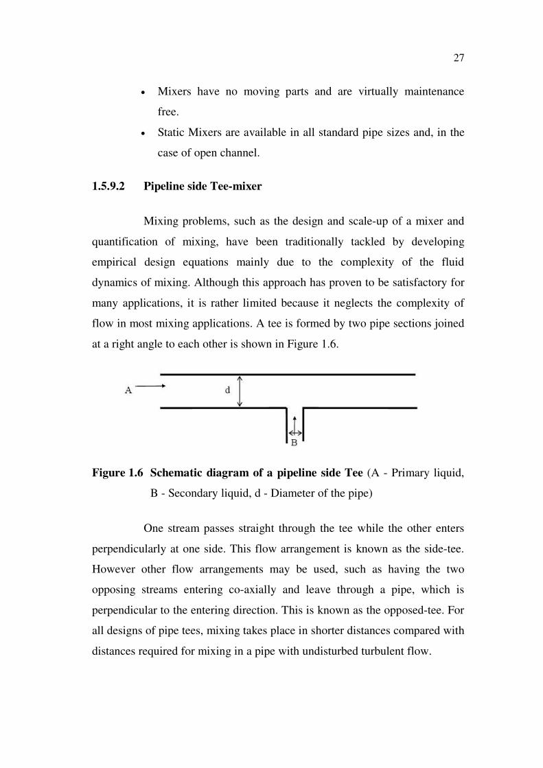
at a right angle to each other is shown in Figure 1.6.

Figure 1.6 Schematic diagram of a pipeline side Tee (A - Primary liquid,

B - Secondary liquid, d - Diameter of the pipe)

One stream passes straight through the tee while the other enters

perpendicularly at one side. This flow arrangement is known as the side-tee.

However other flow arrangements may be used, such as having the two

opposing streams entering co-axially and leave through a pipe, which is

perpendicular to the entering direction. This is known as the opposed-tee. For

all designs of pipe tees, mixing takes place in shorter distances compared with

distances required for mixing in a pipe with undisturbed turbulent flow.

28

1.5.9.3 Active and passive mixers

In general, mixing strategies can be classified as either active or

passive, depending on the operational mechanism.

Active mixers

Active mixers like stirring tanks employ external forces, beyond

the energy associated with the flow, in order to perform mixing. A distinct

advantage over passive type mixers is that these systems can be activated on-

demand. While generally effective in generating turbulence for rapid fluid

mixing in short length-scales, these designs are often not easy to integrate

with the in line process equipments and typically add substantial complexity

in the fabrication process. Moreover, since high electric fields, mechanical

shearing, or generation of nontrivial amounts of heat are involved, they are

not well suited for use in applications involving sensitive species (e.g.,

biological samples).

Passive mixers

Passive mixers, on the other hand, avoid these problems by

exploiting characteristics of specific flow fields to mix species without

application of external electrical or mechanical forces. These gentle designs

are also often more straight forward to build and interface with in line process

equipments.

In static mixers, especially turbulent jet mixers, mixing

preliminarily depends on the formation of counter rotating vortex pair and

turbulent intensity. As a consequence, the distance it would take to obtain a

uniform mixing of two liquids across the mixer, may require a long distance

depending on the jet to crossflow momentum ratio involved (Monclova and

Forney 1995, Maruyuma et al. 1982).

29

This problem has motivated several researchers, over the last few

decades, to design an appreciable number of passive mixers. Among these,

venturi-jet mixers are the most efficient ones, the reasons being that venturi

shape provides exponential growth of the contact interface between two

liquids and entrainment of tracer due to suction effect.

1.5.10 Venturi-jet Mixers

The use of venturi-jet mixers in continuous processes is an

attractive alternative to conventional agitation since similar and sometimes

better performance can be achieved at lower cost.

As they have no moving parts, venturi-jet mixers typically have

lower energy consumptions, smaller space requirements, low equipment cost

and reduced maintenance requirements compared with mechanically stirred

mixers as shown in Figure 1.7. They offer a more controlled and scaleable

rate of dilution in fed batch systems and can provide homogenization of feed

streams with a minimum residence time. They also provide good mixing at

low shear rates where locally high shear rates in a mechanical agitator may

damage sensitive materials.

Figure 1.7 Mechanical stirred tank mixers (Bakker et al. 2001)

30

1.5.10.1 Entrainment mechanism in a venturi tube

The converging tube is an effective device for converting pressure

head to velocity head, while the diverging tube converts velocity head to

pressure head. The two may be combined to form a venturi tube, named after

Venturi, an Italian, who investigated this principle in 1791. It was applied to

the measurement of water by Clemens Herschel in 1886.

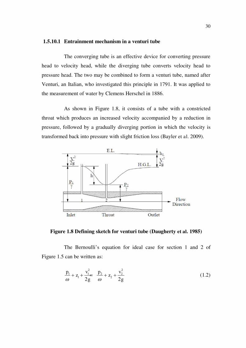
As shown in Figure 1.8, it consists of a tube with a constricted

throat which produces an increased velocity accompanied by a reduction in

pressure, followed by a gradually diverging portion in which the velocity is

transformed back into pressure with slight friction loss (Bayler et al. 2009).

Figure 1.8 Defining sketch for venturi tube (Daugherty et al. 1985)

The Bernoulli’s equation for ideal case for section 1 and 2 of

Figure 1.5 can be written as:

2 2

1 1 2 21 2

2 2

p v p vz z

g g (1.2)

31

where 1 and 2 are subscripts indicating points 1 and 2; p1 and p2 are pressures;

is specific weight; z1 and z2 are elevations; v1 and v2 are velocities and g is

gravitational acceleration.

Since z1 = z2, Equation (1.2) may be written as:

2 2

2 1 1 2

2 2

p p v v

g g (1.3)

The venturi effect happens due to pressure drop in the throat

portion as velocity in the throat portion increases. The increase in velocity v2

through the throat portion of the venturi tube, as a result of the differential

pressure, results in a decrease in pressure p2 in the throat portion (Daugherty

et al. 1985).

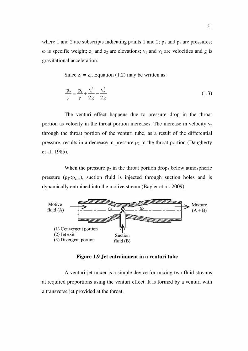
When the pressure p2 in the throat portion drops below atmospheric

pressure (p2<patm), suction fluid is injected through suction holes and is

dynamically entrained into the motive stream (Bayler et al. 2009).

Figure 1.9 Jet entrainment in a venturi tube

A venturi-jet mixer is a simple device for mixing two fluid streams

at required proportions using the venturi effect. It is formed by a venturi with

a transverse jet provided at the throat.

32

One fluid stream (motive fluid or crossflow) passes through the

venturi while the other stream (suction fluid or secondary fluid or jet fluid)

enters through jet into a venturi due to low pressure created at the throat of the

venturi as shown in Figure 1.9. The low pressure created at the throat portion

of the venturi due to change in cross section area lead to the proportional

mixing of two liquids.

1.5.10.2 Previous works on venturi-jet mixers

Eric Haliburn invented the venturi-jet mixer in 1924 to rapidly mix

a continuous supply of cementitious grout for cementing oil wells (Mathys

2004).

Collins and Willis (1970) found that a venturi type mixing unit can

also be used for mixing two fluid streams such as water and soil conditioning

fluid such as liquid insecticides, pesticides, fertilizers, or of other stimulants

for plant growth. The mixing characteristics were determined with regard to

mixing ratio.

A venturi device made from standard sizes of polyvinyl chloride

plumbing and rod-stock material was tested at Little Port Walter, an estuary in

southeastern Alaska (William and Frederick 1978). When installed in a

gravity-fed freshwater delivery system, the venturi injected seawater into the

discharge water to produce a stable water flow of intermediate salinity. The

use of interchangeable components with different-sized openings permits

regulation of the salinity of the discharge water.

Stephen et al. (1990) studied the characteristics of siphon-jet flows

for several geometric configurations and flow speeds. A general method for

optimising the design of liquid / liquid jet pumps was suggested by Vyas and

Kar (1972) in which component dimensions (suction nozzle, driving nozzle,

33

mixing tube and diffuser) were expressed as dimensionless ratios. They

described the entrainment of the suction fluid by viscous friction and

acceleration of the resulting mixture by momentum transfer with the driving

fluid in the mixing tube (throat); complete mixing was assumed by the end of

the throat, as is the case with other researchers (Raynerd 1987 and

Bonnington 1964).

In a series of bench mark studies of mixing by Liscinsky and True

(1996), the venturi mixing performance was improved by free stream

turbulence and mainstream swirl. The results were compared for a jet-to-

mainstream momentum flux ratio of 8.5.

Jean-Michel (2005) developed a venturi mixing device to mix

liquid fertilizer with water and suggested that without any manipulation /

adjustment, intimate mixing could be obtained in the course of distribution.

Recently, Baylar and Emiroglu (2003), Emiroglu and Baylar

(2003), Baylar et al. (2005), Baylar and Ozkan (2006), Ozkan et al. (2006)

and Baylar et al. (2007 a, 2007 b) studied the use of venturi tubes in water

aeration systems.

Fahri et al. (2006) investigated pond aeration by two phase flow

systems such as high head gated conduit flow systems and two phase pipe

flow systems using venturi tubes. When the gate of a high head outlet conduit

is partly opened or a minimal amount of differential pressure exists between

the inlet and outlet sides of the venturi tube, air suction occurs at air vents. In

two phase flow systems, air that is entrained into the water will be

momentarily forced downstream in the form of small air bubbles. The

dissolution of oxygen into the water results from the air suction downstream

of high head gated conduit and venturi tube, and the rising air bubbles into

pond.

34

Baylar et al. (2007) investigated the effect of the venturi tubes with

diameters of 36 mm, 42 mm and 54 mm on air injection rate. In the flow of

the fluid through a completely filled venturi tube, gravity does not affect the

flow pattern. Thus, the Reynolds number was used as dimensionless

parameter and varied between 35000 and 437000. They concluded that

venturi tube does not require external power to operate. It does not have any

moving parts, which increases its life and decreases the probability of failure.

The venturi tube is usually constructed of plastic and it is resistant

to most chemicals. It requires minimal operator attention and maintenance. As

the device is very simple, its cost is low. It is easy to adapt to most new or

existing systems provided that there is sufficient pressure in the system to

create the required pressure differential.

In a practical situation, economic considerations will establish the

appropriate compromise involving tank size, jet diameter and flow rate,

venturi and air hole geometry that will lead to optimum aeration efficiency.

1.5.11 Computational Fluid Dynamics Analysis of Mixer

CFD is the science of predicting fluid flow, heat transfer, mass

transfer, chemical reactions, and related phenomena by solving the

mathematical equations which govern these processes using a numerical

process. This technique has become so important that it now occupies the

attention of perhaps a third of all researchers in fluid mechanics and the

proportion is still increasing (Ferziger and Peric 1996).

One of the reasons for its popularity is that it can be used to solve

real world problems. Solving the equations for fluid flow exactly is almost

always impossible, except in some special cases.

35

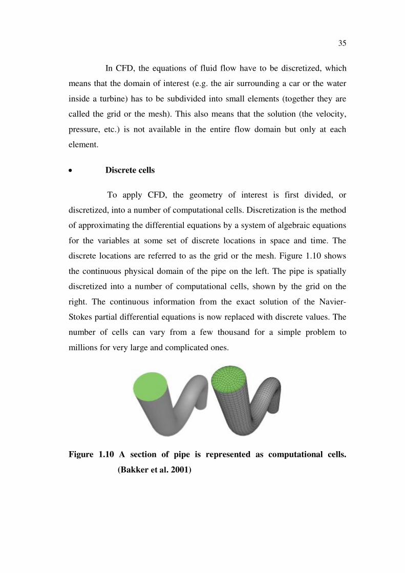
In CFD, the equations of fluid flow have to be discretized, which

means that the domain of interest (e.g. the air surrounding a car or the water

inside a turbine) has to be subdivided into small elements (together they are

called the grid or the mesh). This also means that the solution (the velocity,

pressure, etc.) is not available in the entire flow domain but only at each

element.

Discrete cells

To apply CFD, the geometry of interest is first divided, or

discretized, into a number of computational cells. Discretization is the method

of approximating the differential equations by a system of algebraic equations

for the variables at some set of discrete locations in space and time. The

discrete locations are referred to as the grid or the mesh. Figure 1.10 shows

the continuous physical domain of the pipe on the left. The pipe is spatially

discretized into a number of computational cells, shown by the grid on the

right. The continuous information from the exact solution of the Navier-

Stokes partial differential equations is now replaced with discrete values. The

number of cells can vary from a few thousand for a simple problem to

millions for very large and complicated ones.

Figure 1.10 A section of pipe is represented as computational cells.

(Bakker et al. 2001)

36

Boundary conditions and solution

Once the grid has been created, boundary conditions need to be

applied. Pressures, velocities, mass flows, and scalars such as temperature

may be specified at inlets; temperature, wall shear rates, or heat fluxes may be

set at walls; and pressure or flow-rate splits may be fixed at outlets. The

component material transport properties, such as density, viscosity, and heat

capacity, need to be prescribed as constant or selected from a database. These

can be functions of temperature, pressure, or any other variable of state.

Fluids can be modeled as either incompressible or compressible. The

viscosity of the fluid can be either Newtonian, or non-Newtonian, using the

power law, Herschel-Bulkley, Carreau, or viscoelastic models. In mass- or

heat-transfer applications, binary diffusivities and thermal properties need to

be defined as well. With the grid created, the boundary conditions and

physical properties defined, the calculations can start. The code will solve the

appropriate conservation equations for all grid cells using an iterative

procedure. Typical CPI process problems involve solving for:

Mass conservation (using a continuity equation);

Momentum (using the Navier- Stokes equations);

Enthalpy;

Turbulent kinetic energy;

Turbulent energy dissipation rate;

Chemical species concentrations;

Local reaction rates; and

Local volume fractions for multiphase problems.

It is important to understand that a CFD solution to a particular

problem involves approximations at several levels. The equations being

solved are a model of reality, not reality itself. Secondly, when the equations

are discretized, approximations are introduced. If it was possible to use an

37

infinite number of elements it would be possible to get very close to the exact

solution. But since computers are not infinite fast with infinite memory, there

is a limit on the number of elements that can be used. Therefore we cannot

resolve everything inside the flowing fluid (Baylar et al. 2009).

The actual CFD solving process is often done in steps (iterations)

towards the exact solution. This process has to be stopped at some level which

means that the exact solution to the discretized equations is never reached (but

it is possible to get very close) (Ferziger and Peric 1996).

1.5.11.1 Previous works on CFD analysis of transverse mixers

Mixer design is slowly changing from being a complete

experimental process to a partially numerical and experimental one.

Numerical simulation has an advantage that analysis and optimization can be

done before the device is built. Consequently, the design of new mixing

devices becomes less expensive and at the same time faster.

Chang and Chen (1994) analysed the mixing of opposing heated

line jets discharged normally or at an angle into horizontal cold crossflow

rectangular channel by using k- turbulence model. The results indicate that

turbulence kinetic energy is high in the region where vertical velocity gradient

is steep.

Recently, some numerical studies have been performed on two- or

three-dimensional turbulent mixing with mass or heat transfer for simple

geometries (Monclova and Forney 1995).

There have been several previous efforts to model the flow in

transverse mixers using CFD. Xiaodong Wang et al. (1999) used a

commercial CFD code to analyse the mixing performance of transverse

mixers that was used in a silo unit for the mixing of fibre with water.

38

Diego and Timothy (2004) simulated the effect caused by obstacles

in the throat of the venturi on the flow field of a compressible, steady state,

single phase, fully turbulent flow and mixing using a commercial CFD

package. First, a 2-D axisymmetric geometry was used to study a venturi

without restrictions. Second, a 3-D geometry was used to see the effect of

different diameters and insertion lengths of the fuel tube, as well as the impact

of a secondary fuel tube passing through the venturi throat. The results

showed that obstacles in the throat of the venturi created a recirculation zone

with high turbulence intensity. A larger fuel tube produces stronger

turbulence and larger recirculation zones, while a small secondary fuel tube

creates additional recirculation zones at the top of the venturi that interact

with those at the bottom. These zones may influence secondary droplet

formation and mixing downstream of the venturi.

Veronica and Joel (2004) conducted study to evaluate the use of

CFD for analysing mixing effectiveness of low-energy mixers in water and

waste-water treatment process. In this study CFD was used to predict

downstream mean tracer concentration and segregation intensity in different

closed conduit reactor geometries. Mixing configurations include a plane

shear layer, plane jet in a square conduit, a round jet in a circular conduit, and

a hydraulic jet in a 1- and 6-in. diameter pipe. The results showed that the

multi-fluid model better predicted the mean concentration than the single fluid

model.

The flow and mixing characteristics of three-dimensional confined

turbulent round opposing jets in a Tee mixer, using air as the working fluid

were examined numerically by Wang and Mujumdar (2007). Computational

fluid dynamics (CFD) model was validated with experimental results for a

Tee mixer in which a side stream normally impinges on a main stream. The

effects of key parameters (i.e., jet Reynolds number, dome height, jet

39

injection angle, and side-to-main pipe diameter ratio) on mixing are discussed

for this opposing jet configuration for passive mixing of fluid streams without

the use of internal flow obstructions in the pipe.

Some of the recent advances in applying CFD techniques to the

chemical process industry are documented by Shanley (1996). However, very

few studies are available for dealing with complex three-dimensional

turbulent simulation with mass transfer in venturi-jet mixer.

In addition to experimental and numerical analysis by using natural

coordinate system, the present study also employs CFD technique to elucidate

the flow and mixing characteristics on the transverse turbulent jet flow in

venturi-jet mixer with different injection angles.

Moreover the mixer performance can be predicted, enhanced, and

simulated at various conditions. The some aspects on performance of the

mixers are compared. These will also give us some idea how CFD can help

engineers to improve the mixer performance while saving operating time and

costs due to experiments, although some actual tests are still required.

1.5.11.2 Boussinesq hypothesis

Turbulence is characterized by two parameters: the kinetic

turbulence energy k and the rate of its dissipation . Transfer equations for

these functions are formulated with the use of the Boussinesq hypothesis and

its analogy. This hypothesis underlies most of the engineering calculations of

turbulent flows (Rubel 1985).

An alternative to the Boussinesq hypothesis is separate simulation

of all components of the turbulent-stress tensor, with the result that the

corresponding transfer equation is constructed and solved for each Reynolds

stress.

40

Compared to the turbulent-viscosity based models, such an

approach possesses an important advantage in that it abandons the assumption

of local isotropy, but it contains numerous empirical constants. Found for one

type of flow, they do not necessarily guarantee improvement in the accuracy

of calculation in another; a much larger volume of computations is required.

In the turbulent-viscosity-based models, unknown correlations are

simulated by averaging the flow parameters in closing the equations for

turbulent characteristics.

The Boussinesq hypothesis enables us to write the Reynolds-stress

tensor in terms of the strain-rate tensor of the averaged velocity with

introduction of the notion of a turbulent viscosity t by analogy with the

molecular viscosity lam. In this case for calculation of the turbulent

characteristics Chornyi et al. (2008) have obtained, from the Navier–Stokes

equations, the standard k model.

The turbulent transport of a vector variable, like momentum, and of

a scalar variable, like heat or a species, is not necessarily described with one

diffusion coefficient (Kok and Vander Wal 1996). The ratio of the momentum

to the scalar-diffusion coefficient is given by the turbulent Schmidt number

Sc, where 0.1 < Sc < 1.0.

1.5.11.3 The k- turbulence model

Turbulent flows are commonly encountered in practical

applications. It is the time-mean behaviour of these flows that is usually of

practical interest. The currently popular “two-equation models” of turbulence

(Launder et al. 1974) employ, as one of the equations, the equation for the

kinetic energy k of the fluctuating motion, which reads:

41

. . )k

k uk k Gt

(1.4)

wherek, is the diffusion coefficient for k, G is the rate of generation of

turbulence energy, and is the kinematic rate of dissipation. The quantity G-

is the net source term in the equation. A similar differential equation

governs the variable .

Figure 1.11 Deflected jet situation (Patenkar et al. 1977)

A turbulent jet issuing from a circular orifice that is deflected by a

stream normal to its axis induces a three-dimensional elliptic flow.

An impression of the flow pattern given by Patankar (1980) is shown in

Figure 1.11.

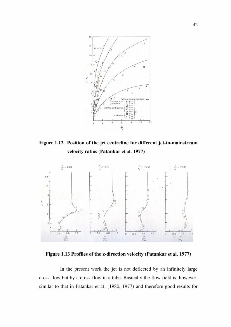
Patankar et a1. (1977) solved numerically the three-dimensional

flow field of the deflected jet on the basis of the k model of turbulence.

Their predictions shown in Figure 1.12 and Figure 1.13, find good agreement

between numerical prediction and experiment (Ramsey 1970, Keffer 1963,

Jordinson 1958).

42

Figure 1.12 Position of the jet centreline for different jet-to-mainstream

velocity ratios (Patankar et al. 1977)

Figure 1.13 Profiles of the z-direction velocity (Patankar et al. 1977)

In the present work the jet is not deflected by an infinitely large

cross-flow but by a cross-flow in a tube. Basically the flow field is, however,

similar to that in Patankar et al. (1980, 1977) and therefore good results for

43

the prediction of flow field and turbulent mixing are expected with the k

model of turbulence. Since Patankar et a1. (1977) also used C = 0.09 this

will most probably predict turbulent mixing of momentum correctly.

1.5.11.4 Definition of turbulence intensity

The turbulence intensity, also often referred to as turbulence level,

is defined as:

'u

IU

(1.5)

where u’ is the root-mean-square of the turbulent velocity fluctuations and U

is the mean velocity (Reynolds averaged). If the turbulent energy,k, is known

can be computed as:

2 2 2' ' ' '1 2

3 3x y z

u u u u k (1.6)

U can be computed from the three mean velocity components Ux, Uy and Uz

as:

2 2 2

x y zU U U U (1.7)

When setting boundary conditions for a CFD simulation it is often necessary

to estimate the turbulence intensity on the inlets. To do this accurately it is

good to have some form of measurements or previous experience to base the

estimate on.

44

Here are a few examples of common estimations of the incoming

turbulence intensity:

High-turbulence case

High-speed flow inside complex geometries like heat-exchangers

and flow inside rotating machinery (turbines and compressors). Typically the

turbulence intensity is between 5% and 20%.

Medium-turbulence case

Flow in not-so-complex devices like large pipes, ventilation flows

etc. or low speed flows (low Reynolds number). Typically the turbulence

intensity is between 1% and 5%.

Low-turbulence case

Flow originating from a fluid that stands still, like external flow

across cars, submarines and aircrafts. Very high-quality wind-tunnels can also

reach really low turbulence levels. Typically the turbulence intensity is very

low, well below 1%.

1.5.11.5 Energy spectrum of turbulent boundary layer

Figure 1.14 gives information about the mean-energy of the

turbulent structures which have the same dimensions. The energetic structures

can be split in the following ranges:

energy-containing range, which contains the largest vortical

turbulent structures

inertial range or sub range, which contains vortices of

intermediate dimensions

dissipation range, which contains the smallest structures.

45

Figure 1.14 Typical energy spectrum of a turbulent boundary layer

To estimate the characteristic time and the characteristic

dimensions of turbulence, the results of the Universal Equilibrium Theory of

Kolmogorov can be used (Kolmogorov). The spatial orders of magnitude of

the largest scales, L, and of the smallest scale in the flow, lk, are related as

follows:

34Re

k

L

l (1.8)

where Re = uL/ is the Reynolds number of the flow, based on L and on an

integral velocity u, which can be assumed similar to the velocity of the largest

scales. It can be seen that the separation between large and small scales

increases with the Reynolds number.

The largest scales of turbulence carry most of the turbulence kinetic

energy so they are responsible of the turbulent transport. The smallest scales

are responsible of most of the dissipation of kinetic energy, so even if their

contribution to the kinetic energy is negligible in comparison with the largest

scales they must be considered to obtain accurate results.

46

1.5.11.6 Fluent solver package

CFD is a tool that uses numerical methods to solve partial

differential equations like Navier Stokes equations and Fick’s Law. In the

present work, CFD is also used to study the JICF and the mass transfer

phenomena generated by the JICF.

Most of the commercial CFD codes (like Fluent), and open-source

codes for multipurpose and complex physics (like Openfoam), are developed

in C and C++. FLUENT is a state-of-the-art computer program for modelling

fluid flow and heat transfer in complex geometries.

FLUENT is written in the C computer language and makes full use

of the flexibility and power offered by the language. Consequently, true

dynamic memory allocation, efficient data structures, and flexible solver

control are all made possible.

FLUENT provides complete mesh flexibility, solving the flow

problems with unstructured meshes that can be generated about complex

geometries with relative ease. Supported mesh types include 2D

triangular/quadrilateral, 3D tetrahedral/hexahedral/pyramid/wedge, and mixed

(hybrid) meshes.

FLUENT also allows refining or coarsening the grid based on the

flow solution. This solution-adaptive grid capability is particularly useful for

accurately predicting flow fields in regions with large gradients, such as free

shear layers and boundary layers.

In comparison to solutions on structured or block structured grids,

this feature significantly reduces the time required to generate a "good" grid.

Solution-adaptive refinement makes it easier to perform grid refinement

47

studies and reduces the computational effort required to achieve a desired

level of accuracy, since mesh refinement is limited to those regions where

greater mesh resolution is needed.

The Navier-Stokes equations are no linear differential equation and

as we have seen, we can solve them numerically using FVM. One of the

issues that have to be faced when the Navier-Stokes equations have to be

solved is the fact that they are equations coupled through them by mean of

variables like velocity, density and pressure and they have to be solved in a

certain order (Salvatore, 2009).

The choice of the algorithm that defines the order in which the

Navier-Stokes equations are solved is a key element in a CFD simulation, and

in the commercial code Fluent there are 2 major numerical solvers; namely,

Segregated solver and Coupled solver – Implicit and Explicit.

Segregated solver

The governing equations are nonlinear and coupled; each governing

equation has to be solved iteratively. Fluent solves the set of equations

sequentially (segregated from the others) or using a coupled system of

equations comprising momentum equations and the pressure based continuity

equation. For this segregated solver was used.

Figure 1.15 gives an overview of the segregated solution method in

the following steps (Aryoso 2007).

1. Fluid properties are updated, based on the current solution.

2. The u, v, and w momentum equations are each solved in turn

using current values for pressure face mass fluxes, in order to

update the velocity field.

48

Figure 1.15 Overview of the segregated solver

3. Since the velocities obtained in step 2 may not satisfy the

continuity equation locally, “Poisson – type” equation for the

pressure correction is derived from the continuity equation

and the linearized momentum equations. This pressure

correction equation is then solved to obtain the necessary

correction to the pressure and velocity fields and the face

mass fluxes such that the continuity is satisfied.

4. Where appropriate, equations for scalars such as turbulence,

energy, species and radiation are solved using the previously

updated values of the other variable.

5. When interphase coupling is to be included, the source terms

in the appropriate continuous phase equations may be updated

with a discrete phase trajectory calculation.

Update properties

Solve momentum equations

Solve energy, species, turbulence and other scalar

equations

Solve pressure corrections (continuity equation.

Update pressure, face mass flow rate

Converged

Stop

49

6. A check for the convergence of the equation set is made.

The iterative process is continued until the convergence criteria are

met.

Coupled solver

The coupled solver solves the governing equations of continuity,

momentum and energy (where appropriate) and species transport

simultaneously (i.e., coupled together). Governing equations for additional

scalar will be solved sequentially (i.e., segregated from one another and from

the coupled set) using the procedure described for the segregated solver above

because the equations are non-linear (and coupled), several iterations of the

solution loop must be performed before a converged solution is obtained.

1.5.11.7 Finite volume method

There are three distinct streams of numerical solution techniques

able to discretize partial differential equation like Navier Stokes equations:

Finite difference method (FDM)

Finite element method (FEM)

Finite volume method (FVM)

All the aforementioned methods can be used to solve numerically

partial differential equations successfully, but according to the complexity of

the phenomena, the importance of coherently describe the conservation laws

evocated by the equation itself and the computational capability available, is

better to implement one method or another.

In the case of fluids the equation to be solved are the Navier Stokes

equations, and the methods that more coherently maintains the conservation

50

of all variable is the FVM. That’s why most of the CFD codes are based on

FVM.

The conservative form of all fluid flow equations, including

equations for scalar quantities ( ) such as temperature and concentration etc.,

can usefully be written in the form:

. u St

(1.9)

The steady conservation equation in integral form to discretize the

governing equations by finite volume method for transport of a scalar quantity

in a control volume V from Equation (1.9) is written as:

. V

u dA S dV (1.10)

where = density,

u = velocity vector

A = surface area vector

= diffusion coefficient for

= gradient of

S = source term of per unit volume

The space discretization of the Equation (1.10) for a steady flow

problem on a given cell can be done with:

.f f f f fu A S V (1.11)

A linearized discretized transport equation for the scalar quantity

can be written using the following formulation:

51

p nb nb

nb

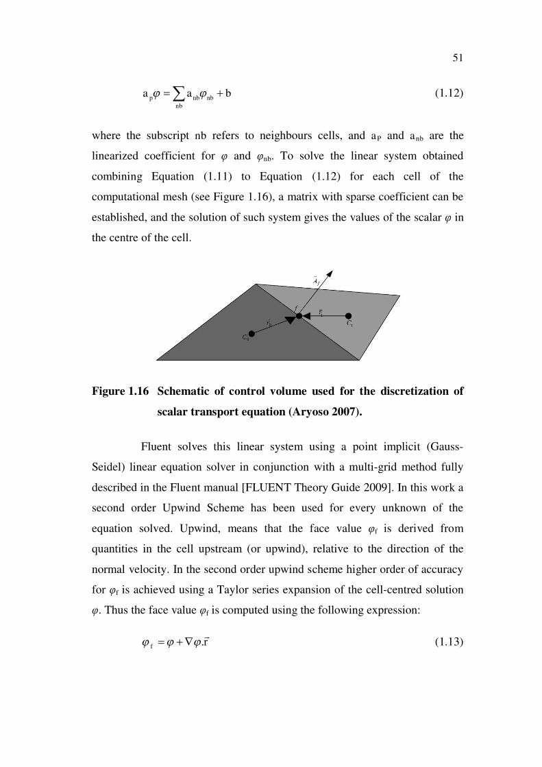
a a b (1.12)

where the subscript nb refers to neighbours cells, and aP and anb are the

linearized coefficient for and nb. To solve the linear system obtained

combining Equation (1.11) to Equation (1.12) for each cell of the

computational mesh (see Figure 1.16), a matrix with sparse coefficient can be

established, and the solution of such system gives the values of the scalar in

the centre of the cell.

Figure 1.16 Schematic of control volume used for the discretization of

scalar transport equation (Aryoso 2007).

Fluent solves this linear system using a point implicit (Gauss-

Seidel) linear equation solver in conjunction with a multi-grid method fully

described in the Fluent manual [FLUENT Theory Guide 2009]. In this work a

second order Upwind Scheme has been used for every unknown of the

equation solved. Upwind, means that the face value f is derived from

quantities in the cell upstream (or upwind), relative to the direction of the

normal velocity. In the second order upwind scheme higher order of accuracy

for f is achieved using a Taylor series expansion of the cell-centred solution

. Thus the face value f is computed using the following expression:

.f

r (1.13)

52

The Green Gauss cell-based formulation of gradient is obtained

from the arithmetic average of the values at neighbours’ cell centres:

2

o oc c

f (1.14)

The Green-Gauss cell-based formulation is obtained from the

arithmetic average of the all nodal values Nf on the face.

1 fN

f n

nN (1.15)

where nodal value n is obtained from the weighted average of the cell values

surrounding the nodes. This method proposed by Holmes and Connel

[FLUENT Theory Guide, 2009] reconstruct exact values of a linear function

at a node from surrounding cell centred values on arbitrary unstructured

meshes by solving a constrained minimization problem, preserving a second

order spatial accuracy. For the present study, the Green Gauss node based

method used for accuracy, even in highly skewed cells, even those is

computationally more expensive than the cell based gradient scheme.