chapter 1 introduction - digital.library.adelaide.edu.au€¦ · 2 chapter 1. introduction...
TRANSCRIPT

Chapter 1
Introduction
1.1 On meteors and meteoroids
Meteors are generally described as an atmospheric phenomenon caused by the entrance
of particles from space (meteoroids or space debris) into the earth’s atmosphere. Other
planets or moons with atmospheres should experience similar phenomena, which would
also be labelled meteors. Planets for which the effects of meteors have been investigated
include Neptune (Moses 1992, Lyons 1995), Jupiter (Grebowsky 1981, Kim et al. 1998),
and Mars (Shafrir 1967, Flynn & McKay 1990, Davis 1993, Adolfsson et al. 1996,
Pesnell & Grebowsky 2000), as well as a moon of Saturn, Titan (Ip 1990, Molina-
Cuberos et al. 2001). These particles from space heat up due to collision with air
molecules, and when they reach a high enough temperature, lose atoms and molecules
by evaporation, a process called ablation. Subsequent collision of the meteoroid atoms
and molecules with air molecules produces excited meteoroid atoms and ionisation.
These excited atoms lose energy by emitting light, and as the meteoroid travels through
the atmosphere, it produces a long column of ionisation and luminosity.
The smallest body which will ablate, producing a meteor, depends on its composi-
tion and speed, but a size of ten microns is about the limit. If the particle has sufficient
mass to survive to the ground, it is termed a meteorite.
Most meteoroids enter the atmosphere with speeds greater than 11.2km s−1 (the
1

2 CHAPTER 1. INTRODUCTION
earth’s escape velocity) and ablate at heights between 70 km and 140 km. The upper
limit to the speed of encounter with the earth for a particle in the solar system is
72.8 km s−1, a combination of the solar escape velocity at one Astronomical Unit, 42.5
km s−1, and the orbital speed of the earth, 30.3 km s−1. The few meteors observed
with speeds greater than 72 km s−1 are part of a group called hyperbolic, since their
speed is greater than allowed for a bound heliocentric orbit. Taylor et al. (1994)
show that about 1-2 percent of meteoroids are in hyperbolic orbits and most of these
meteoroids are of interstellar origin. Of course the orbital speed and the meteoroid
speed are added as vectors (velocities), and hyperbolic meteoroids can be observed with
geocentric speeds lower than 72.8 km s−1, however they cannot be distinguished by
geocentric speed alone. Most meteoroids, however, enter the atmosphere with speeds
between 15 and 35 km s−1.
The meteor influx can be divided into shower and sporadic components. Shower
meteors are those associated with a stream of particles (meteoroids) in closely related
orbits, usually from a common source. These streams are almost certainly produced
by comets. When the Earth passes through one of these streams, there is a sharp
burst of meteor activity. For older streams, in which the meteoroids have spread out
in their orbit around the sun, this occurs annually, for example the April/May η-
Aquarids, or the October Orionids. The streams are named for the position in the
sky (or constellation), called the radiant, from which the associated meteors appear to
originate, although these constellations have nothing to do with the formation of the
meteoroid streams.
On the other hand, sporadic meteors are caused by meteoroids in relatively random
orbits colliding with the Earth, and as such are observed as a random background of
activity. These are generally thought to have origins in parts of meteoroid streams
which have been gravitationally perturbed, or in collisions amongst asteroids; there are
four broad apparent sources, corresponding to the Sun (Helion), Antisun (Antihelion),
Apex and Toroidal directions. These sources will be discussed more in Chapter 7. The
journey of a meteoroid on a collision course with the earth is as follows: the particle’s

1.1. ON METEORS AND METEOROIDS 3
motion through space is mostly determined by the gravitational influence of the Sun,
perturbed by close approaches to large bodies such as planets (predominantly Jupiter).
Collisions, the Poynting-Robertson effect, and radiation pressure, have a small but
pervasive effect; further, as it approaches the earth, the local gravitational field causes
a minor perturbation to its path.
As the particle enters the upper atmosphere, the surface temperature rises very
rapidly due to collisions with air molecules. This atmospheric drag also causes the
particle to decelerate. If the particle is very small, smaller than about ten microns
across, then thermal emission tends to balance impact energy gains, and it may be
slowed down to terminal velocity before the onset of ablation. This particle will settle
down through the atmosphere unchanged. Larger particles, up to about 100 microns,
will be large enough to gain more heat than they emit, but small enough for the
heating to be nearly isothermal. For particles greater than about 100 microns in size,
the rate of heat transfer through the particle is too slow to maintain the temperature
equilibrium throughout the particle. Thus a radial temperature gradient is built up
and can lead to fragmentation when the heat stresses become larger than the tensile
strength of the material.
As the temperature rises the surface of the meteoroid begins to sputter, and then
evaporate, the rate of mass loss increasing with temperature. The temperature increase
slows and then stops as the particle ablates, because heat loss due to evaporation
balances the heat gain from collisions. Meteoroids that are loose conglomerates of
small particles and/or ice 1, are likely to break up into pieces before the onset of
ablation, each piece behaving like an individual particle. Deceleration of the body
increases as the surface area to mass ratio increases due to mass loss.
If the body is very large, and/or has a very high speed then the meteor trail may
be bright enough to be classed as a fireball, (-8 magnitude or greater). If the body
is subject to gross fragmentation, then the sudden rise in surface area can lead to a
1These conglomerations of ice and dust are commonly referred to as “Dirty Snowballs”, and are
thought to be of similar composition to cometary nuclei

4 CHAPTER 1. INTRODUCTION
brightening of more than one magnitude, known as a flare. Deceleration rises rapidly
toward the end of the meteor path, and if there is still some mass left when the speed
drops below about 3 km s−1 the particle no longer has enough kinetic energy to sustain
ablation and cools quickly, decelerating to it terminal velocity, and striking the ground,
becoming a meteorite.
If the body is extremely large, greater than about 100m across, it may hit the
ground without being slowed down appreciably and will form an explosive crater as
the massive amount of kinetic energy is liberated on impact. Slightly smaller bodies
may fail to reach the ground, but penetrate the atmosphere to within 10 km of the
surface of the earth and then explode due to fragmentation caused by aerodynamic
stresses. These extremely large bodies would produce destruction on the scale of
nuclear weapons, with massive loss of life and climate changing effects.
1.2 Observation techniques
It is clear from historical accounts that meteors have been observed with the unaided
eye for many centuries, and are recorded by Chinese and Japanese historians (Imoto
& Hasegawa 1958, Hasegawa 1993) as early as 687 BC. Greek and Roman writers
recorded that meteorites were stones falling from space and meteors were sent by the
gods, but by the middle ages the scientific community were convinced that meteors
had a terrestrial origin. It wasn’t until 1798 when two students at the University of
Gottingen, Brandes and Benzenberg, observing meteors simultaneously from separate
locations, demonstrated that the meteors were a terrestrial phenomenon high in the
atmosphere with an astronomical origin. These students were the founders of modern
meteor observing techniques, but it took the spectacle of the 1833 Leonids meteor
storm to create public interest and arouse scientific attention, thus beginning the
science of meteor astronomy.

1.2. OBSERVATION TECHNIQUES 5
1.2.1 Optical techniques
For many centuries, the naked eye was the only method that could be used to observe
meteors. Simple counting of the number of meteors seen in a certain time interval to
give an “hourly rate” was the main purpose of these observations. There were many
groups and individuals making visual observations in the nineteenth century, and
Schiaparelli, Newton and others gathered and interpreted these data, using accurate
observations of the radiants and estimates of speeds to determine the spatial orbits of
meteoroids, in addition to the count rates (Lovell 1954). Hundreds of meteor showers
were recorded in this time. Denning (1899) lists more than 4000 radiants. The true
number of meteors visible, as compared with the number recorded by an observer was
investigated thoroughly by Opik (1922) by the use of double counting. By estimating
the effect of the properties of the human eye, he produced effective fields of view and
collecting areas for a visual observer. Opik also devised a rocking mirror apparatus
which allowed meteor velocities to be estimated visually (Opik 1934). Unfortunately,
his deduction that as many as 70 percent of meteoroids were in hyperbolic orbits was
fallacious.
With the development and utilisation of telescopes, spectrographs, and photogra-
phy, in the 1930’s, and by video, in the 1970’s, the field was expanded from visual
techniques to optical techniques. Telescopic observations increased the limit of de-
tectability from the fifth magnitude limit for unaided eye to the twelfth or thirteenth
magnitude, but much reduced the field of view. Most of the first photographs of mete-
ors were on plates which were exposed for other reasons, but the data obtained was so
useful that dedicated meteor cameras with rotating shutters were introduced at Har-
vard in 1932, most notably used by Whipple (1938) who introduced pairs of cameras to
obtain doubly photographed meteors. These early photographic techniques produced
high precision data, but were unable to record meteors fainter than magnitude zero.
This led to the development of the Super Schmidt cameras, (Whipple 1949), which
used a system of spherical lenses and mirror to increase the sensitivity of the camera to
6 CHAPTER 1. INTRODUCTION
about the fourth magnitude while retaining a field of view of about fifty five degrees.
This system was an enormous step forward in meteor astronomy, allowing highly accu-
rate data to be obtained from a large number of meteors (McKinley 1961). This type
of system has been extensively used but relatively few meteor orbits were obtained.
A total of 1403 precisely reduced orbits were calculated from about 8000 doubly pho-
tographed Super-Schmidt meteors, as well as number of graphically reduced orbits
(Lindblad, private communication). An intensive program of double station photog-
raphy was started in 1951 in Czechoslovakia (Ceplecha 1957) using 30 cameras. This
program continued until 1977, and the observations included a photograph of a very
bright fireball, magnitude -19 in 1959. Predictions made from the data gained from
the photographs led to the discovery of four meteorites (Ceplecha 1961). This led
to the establishment of several photographic fireball networks in Europe and North
America. In recent years, serious amateur astronomers have carried out much meteor
photography and their work is published regularly.
By placing a prism or grating in front of a camera, a spectroscopic photograph could
be taken, and this produced valuable data not only on the composition of meteoroids
but also, in combination with measurements of decelerations their density by deter-
mining the abundances of the elements and molecules detected. The most prominent
features in meteor spectra are emission lines and the commonest and brightest lines
are those corresponding to sodium and magnesium neutral atoms. Other lines which
have been detected are calcium, iron, chromium, lithium, silicon, titanium, manganese,
cobalt, aluminium, nickel, strontium, nitrogen, oxygen, and oxides of these elements.
The spectra of meteor trains are quite different, generally composed of recombination
and forbidden transition lines of oxygen and sulphur.
While photoelectric devices were used in a limited way for meteor observation, both
on their own and in addition to radio and visual observations (McKinley 1961), the
introduction of video cameras has put a new complexion on photographic meteor ob-
servation. The first of these was by Clifton (1973). Since video cameras typically take
an image twenty five times per second, very good time resolution is possible enabling

1.2. OBSERVATION TECHNIQUES 7
velocity and orbit calculations. The introduction of low light level television (LLLTV)
has improved the sensitivity of this technique, with limiting apparent magnitudes of
about +9. Hawkes et al. (1993) have shown that average two station TV meteor sys-
tems are more accurate than typical meteor radars without the biases against high
altitude meteors caused by rapid diffusion. Television systems, however tend to have
small fields of view ( about 15 degrees) and have poor signal to noise, which restrict
observations to clear dark nights. Television has been also been used to record spectra.
Intensified CCD detectors have been used to observe meteors (Hawkes & Jones 1986),
and with the introduction of a mechanical rotating shutter to produce short duration
intensified CCD detectors which have been used to detect the presence (Robertson
& Hawkes 1992) or absence (Shadbolt & Hawkes 1995) of meteor wakes, the visible
luminosity visible immediately behind the meteoroid body.
1.2.2 Radio techniques
Pioneer workers in the 1930’s studying the reflection of radio waves from the ionised
layers of the atmosphere noted sudden increases in the electron density of the E re-
gion during the night, when the sun’s influence could not be contributing. Nagoaka
(1929) seems to have been the first to suggest that meteors could be causing enough
disturbance to affect radio propagation. Schafer & Goodall (1932), along with Skellett
(1935) produced convincing evidence that meteors were causing some of the ionisa-
tion increases at night, noting visual correlation of meteors with sudden ionisation
increases. At about the same time bursts of radio signals were received from trans-
mitters at great distances when the frequency was such that signals were not normally
received beyond the range of the ground ray, and the sky wave would penetrate the E
and F regions. Pierce (1938) suggested that this could be caused by meteor ionisation
but it wasn’t until the great advances in radio and radar technology during the Second
World War that radio meteor astronomy moved out of it’s infancy.
Much of the initial post war meteor research was carried out at Jodrell Bank,
near Manchester, U.K. with modified radars which had been used during the war.
8 CHAPTER 1. INTRODUCTION
There was a rapid development of several techniques including continuous wave (CW)
and pulsed transmissions; single and multiple spaced receivers; and forward-scatter
and back-scatter propagation. Modified wartime radars were also employed at sites
in the USA, Great Britain and Canada. The first big test of the new techniques
was the return of the Giacobini-Zinner comet in 1946 and the associated Giancobinid
meteor shower. Radar observations can be performed in all weather conditions (except
thunderstorms) and during sunlit and moonlit hours, meaning that daytime meteor
showers were soon discovered. Many of these new radars were able to detect meteors
fainter than the visual limit, and the number of meteors recorded rapidly increased.
A meteor head echo2 was first recorded by Hey et al. (1947) who used it to determine
the speed of the meteoroid. Three station observations of head echoes were used to
determine meteoroid orbits (McKinley & Millman 1949), but the use of head echoes for
speed and orbit calculations languished due to low head echo rates and low precision.
The use of head echoes was revisited in the 1990’s using narrow beam radars (Cervera
et al. 1997, Elford 2001a) and the author’s exploitation of them will be expounded
later in this thesis.
Following a suggestion by Herlofson, Ellyett & Davies (1948) developed a new
method to determine meteor speeds by using the radio Fresnel diffraction patterns
that are observed as meteor trails are formed. Many new meteor radars were built in
the fifties and sixties, including two near Adelaide and in Canada, England, Germany,
Czechoslovakia, the USSR, the USA, Sweden, Italy, and New Zealand. These radars
conducted great meteor surveys, covering both hemispheres. These led to the discovery
of many minor and daytime showers and shed light on the distribution of the sporadic
population of meteors. More on modern radio techniques will be covered in later
chapters.
2A head echo is when only a short section of ionisation around the meteoroid body is observed,
and not the ionised meteor trail

1.2. OBSERVATION TECHNIQUES 9
1.2.3 Direct detection and satellite techniques
There have been some attempts to directly detect meteoroids. The first attempts were
by exposing sticky surfaces on aircraft, resulting in the discovery of small shiny spheres
ranging from 1 to 100 microns in diameter which were supposed by Krinov & Fonton
(1954) to be refrozen droplets spattered from large meteors during ablation. Collection
of meteoric particles have been made using collectors on balloons (Coon et al. 1965).
Meteoric particles have been collected in the stratosphere with high flying aircraft, and
have been recovered from polar ice and deep sea sediments; there has been detailed
analysis of the properties of these particles (Jessberger et al. 2001). Other particle
collections made with aircraft bring the particles directly into a mass spectrometer for
compositional analysis (Schwieters et al. 1991).
Other direct detection experiments have attempted to collect or record meteoroids
before they enter the Earth’s atmosphere. Examining the exposed surfaces of space
vehicles for pitting or etching, and various instruments which measure impact during
flight gave records of meteoroid numbers and size. These include microphones to pick
up the sounds of impacts, breaking of wire grids, puncturing pressurised chambers, or
impacting on thin metallic foils. These measurements are important as they detect
meteoroids with much smaller sizes than other means, and do not suffer from the
selection effects inherent in remote sensing techniques, notably ionisation efficiency,
luminosity efficiency and diffusion of ionisation. Many impacts were evident in the
sheets of aluminium foil carried on the NASA Long Duration Exposure Facility which
was in Earth orbit from 1984 to 1990, recovered from space by the Space Shuttle.
A key observation occurred in 1986 when the European Space Agency’s Giotto
probe flew within 600 km of Comet Halley, carrying, among other instruments, me-
teoroid impact detectors, and going on to Comet Grigg-Skjellerup in 1992 providing
valuable information about these comets and the cloud of meteoroids that had been
ejected from them (McDonnell et al. 1993).
Since 1972, instruments on US Department of Defence satellites have been detecting

10 CHAPTER 1. INTRODUCTION
the bright flashes associated with the ablation of large meteoroids. The sensors detect
in both the optical and infrared regions of the spectrum and are able to detect these
fireballs during daylight or the night. They have detected bolides with a peak absolute
brightness of -17.5 . Over 500 events have been recorded and analysed by Nemtchinov
et al. (1997).
1.3 Thesis overview
This chapter has given a short definition of a meteor, and an overview of different tech-
niques used to observe meteors. This thesis concentrates on observations made with
a narrow beam VHF radar, and subsequent analysis of those observations, especially
relating to the structure of meteor showers.
Chapter 2 gives a description of the Adelaide VHF Radar system, its location,
layout and operation as a background to the meteor observations. The antenna pattern
is discussed, as is the beam steering possible with the radar and the effect of using
various values of Pulse Repetition Frequency on the height coverage of the radar. In
addition the format of the recorded data is described and a detection algorithm is
developed.
In Chapter 3, we give a background on the physics of meteor observations with
radar, including ablation theory and radar backscatter. Various attenuation factors
and the effect of the geomagnetic field on the diffusion of the meteor are examined,
and the radar response function is derived and examined.
Chapter 4 details how the recorded data is processed, including coherent smoothing
of the data, the removal of periodic noise and unwrapping of the phase data. The
effects of receiver saturation are examined to determine the extent of errors caused by
saturation.
We see an examination in Chapter 5 of the types of echoes observed, including
transverse, down-the-beam and head echoes, as well as periodic noise and aircraft

1.3. THESIS OVERVIEW 11
echoes. We look as the occurrence rates of each of the types of echo. Much infor-
mation is available in the data recorded including meteor heights, radial wind speeds,
fragmentation, diffusion rates and the physical properties of meteoroids.
Chapter 6 looks at new methods of determining meteoroid speeds which are ap-
plied to three different types of meteor echoes as well as a review of previously and
currently used methods. The measurement of the deceleration of meteoroids is exam-
ined, and a comparison of the pre-t0 phase method and the Fresnel Transform methods
of determining meteor speeds shows good correlation.
In Chapter 7 we look at the structure of meteoroid streams. First an overview of
previous meteor shower observations, models of stream formation and evolution. A
description of the radar response function method for observing meteor showers and
a discussion of random meteor count rate statistics follows, then detailed observations
of meteor showers and how they pertain to meteoroid stream structure, concentrating
mainly on the η-Aquarid meteor shower. These observations include instantaneous
meteor count rates and distributions of meteor speeds and heights. An examination
of the Orionid and Leonid meteor showers follows, and then the sporadic background
is discussed.
Chapter 8 gives conclusions and suggestions for further work.

12 CHAPTER 1. INTRODUCTION
Chapter 2
The Buckland Park VHF Radar.
2.1 Introduction
The Buckland Park (BP) VHF Radar is situated at a University of Adelaide field
station located about 35 km north of Adelaide (3437′S , 13829′E), near a rural
property named “Buckland Park”, hence the naming of the field site, and the radar.
The field station is about 2 × 2 km, and the radar is situated in the southeastern
corner of the site. Also at the station are an MF (1.98 MHz ) radar, which has an
array size of 1 × 1 km (Briggs et al. 1969) and a 54.1 MHz Boundary Layer radar
(Vincent et al. 1998). Since the VHF radar also operates at 54.1 MHz, it and the
Boundary Layer radar must operate at different times to avoid interference. The VHF
radar is ideal for radar observation of meteors, although it was originally designed for
studies of the lower atmosphere, specifically to study vertical profiles of tropospheric
winds (Vincent. et al. 1987). The radar initially consisted of a 90×90 m array, known
as the East-West Array1 as the antennas were in North-South aligned rows. A set of
East-West rows were later added, known as the North-south array.
Since the potential of the radar for meteor observation was realised, it has been used
to investigate meteor height distributions (Steel & Elford 1991), meteor shower radiant
1The two arrays are named for the direction in which they can direct the radar beam. Thus, the
East-West array produces beams which can be directed at a range of elevations in the East-West
plane; similarly for the North-South array
13

14 CHAPTER 2. THE BUCKLAND PARK VHF RADAR.
Wavelength 5.545 m
Frequency 54.1 MHz
Pulse width 12.8 µsPulse repetition frequency (PRF) 2000 Hz
Peak power 24 kW
Off zenith angle 30
Range bin size 2 km
Sampling start height (range) 68 km (79 km)Sampling end height (range) 129 km (149 km)
Table 2.1: Typical operational parameters used for meteor observations.
determinations (Elford et al. 1994), meteor drift wind speed measurements (Cervera
& Reid 1995), meteoroid speed measurements (Elford et al. 1995), meteor deceleration
measurements (Taylor et al. 1996) and measurements of the Faraday rotation of meteor
echoes (Elford & Taylor 1997). The radar has been upgraded several times over this
period. Recent upgrades include the installation of a new transmitter (April 2000),
a new Radar Data Acquisition System (RDAS) and a North-South array (1996), and
the new beam steering hardware (1997). The radar has also undergone several repairs,
notably to the receivers and beam swinging gear after a lightning strike in 1998 and
to the transmitter after a cooling system water leak also in 1998. The damage caused
by the leak could not be completely repaired, and the radar was running with reduced
peak power until the new transmitter was installed in 2000. Table 2.1 shows the
operational parameters typically used for meteor observations.
2.2 Layout and Operation
The antenna system consists of two orthogonal coaxial-collinear (CoCo) type antenna
arrays, and each can be used for both transmission and reception. It covers an area
about 90 × 90 m. The East-West array which consists of 32 North-South rows, each
consisting of 48 dipoles, and the North-South array, added in 1997, which consists of
two sets of 32 East-West rows, each containing 22 dipoles. A CoCo antenna is a length

2.2. LAYOUT AND OPERATION 15
4
N (true)
Ground PlaneWires
Radar Building Receivers Data recording
Transmitter Caravan
Feed point from Transmitter
Figure 2.1: The layout of the Adelaide VHF Radar (after (Hobbs 1998) )
of 52 Ω coaxial cable with the inner and outer conductors interconnected every half
wavelength (Wheeler 1956). That is, the inner conductor of one section is connected
to the outer conductor of the next, and vice versa. This type of array is cheap to build
and maintain, so they are widely used, despite their efficiency being lower than the
efficiency of Yagi arrays (about 30 percent for the VHF versus about 80 percent for a
similar Yagi array). The array is actually oriented 4 degrees west of True North, as
seen in Figure 2.1. This makes it parallel with the MF radar array on the site, which

16 CHAPTER 2. THE BUCKLAND PARK VHF RADAR.
N
E
S
W
(a) (b)
(c) (d) (e)
Figure 2.2: Array configurations for interferometric observations. (a) uses the East-West array and (b) to (e) are using the North-South array.
was aligned this way to match the site boundaries. There is a 1.5 wavelength gap
in the centre of the array, along the rows of the East-West antennas, which contains
a caravan containing the transmitter and beam swinging gear. The other rows are
separated by half a wavelength. The array is situated a quarter wavelength above
the ground, which has a ground plane laid on it composed of copper wire spaced one
quarter of a wavelength apart in both directions. This ground plane makes the antenna
independent of the reflectivity of the ground. To the east of the array lies the VHF
hut, containing the receivers, the RDAS, the RDAS controlling PC, and the Meteor
data acquiring PC.
The two arrays produce a beam with a half width at half power beam of about
1.8 degrees for the East-West antennas and about 1.7 degrees for the North-South
antennas. The difference is due to the slightly different construction of the two arrays.
The pattern is also asymmetric due to the gap between the rows for the transmitter
caravan. These narrow beams and the peak power of 32 kW mean that meteors as

2.3. ANTENNA PATTERN. 17
Figure 2.3: The one way antenna pattern for the East-West array for a 30 tilt east-wards as derived by Cervera (1996). (a) and (b) show the cross sections of the antennapattern in the North/South and East/West planes respectively. See text for furtherdetails
faint as +13.5 magnitude can be detected, corresponding to an electron line density of
∼ 1011em−1. The narrow beam also allows accurate determination of meteor shower
radiants. These two properties give the Adelaide VHF radar significant advantages
over conventional wide-beam meteor radars. Another advantage over many other
meteor radars is the ability to record both phase and amplitude data, which enables
detailed information to be obtained about the formation of the trail, and in particular,
allows the calculation of wind drifts and meteoroid speeds as detailed in Chapters 4 and
5. Both arrays can be split into sections in order to make interferometric observations
of the received signals. These sections are shown in Figure 2.2.
2.3 Antenna pattern.
It is important for experimental work that the antenna pattern of the array is well
known. Cervera (1996) covers in detail a theoretical derivation of the antenna pattern
for the East-West Array including the effects of factors such as an imperfect ground
18 CHAPTER 2. THE BUCKLAND PARK VHF RADAR.
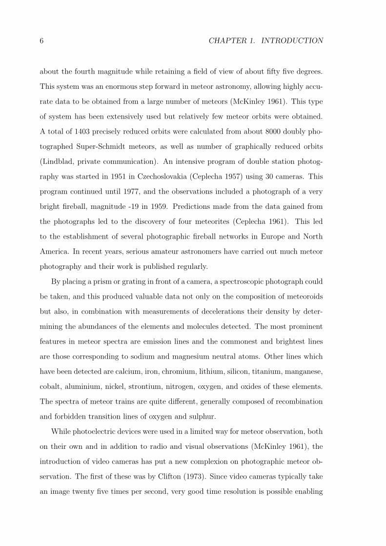
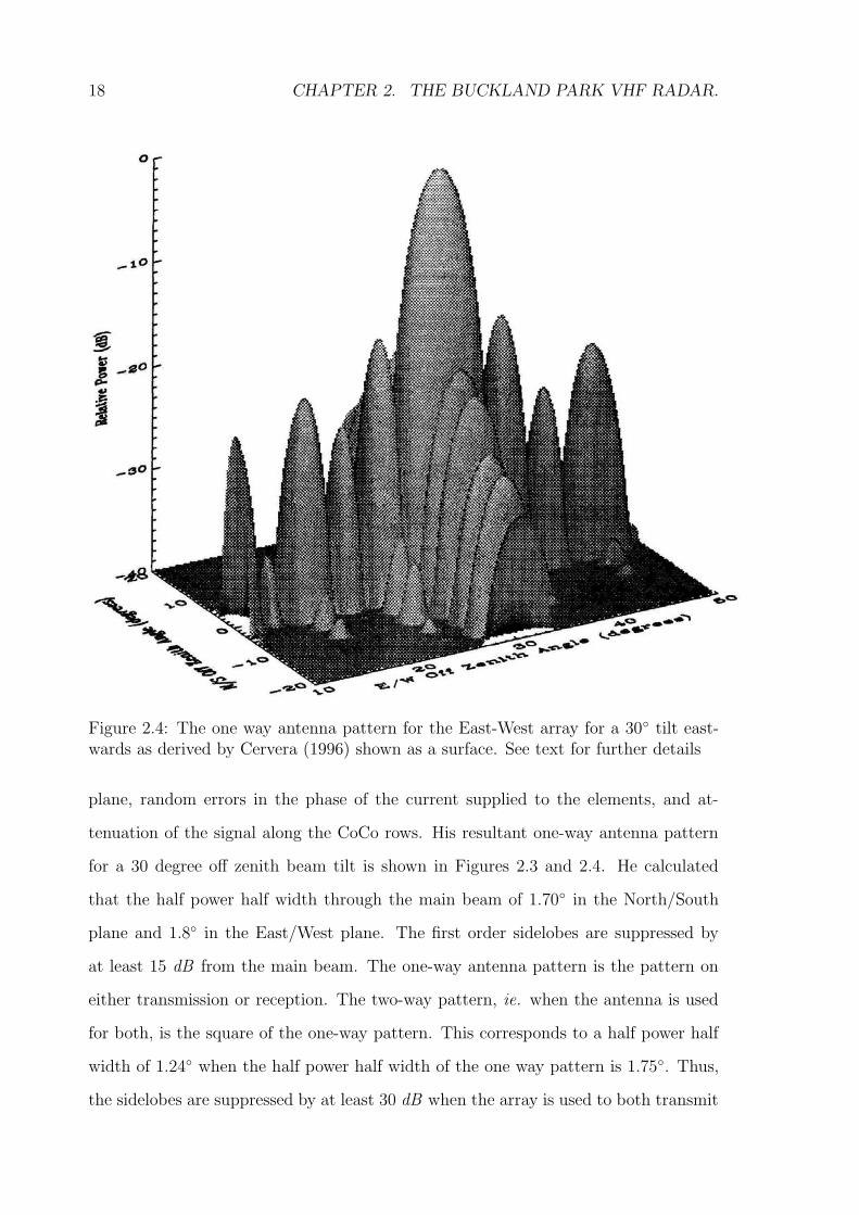
Figure 2.4: The one way antenna pattern for the East-West array for a 30 tilt east-wards as derived by Cervera (1996) shown as a surface. See text for further details
plane, random errors in the phase of the current supplied to the elements, and at-
tenuation of the signal along the CoCo rows. His resultant one-way antenna pattern
for a 30 degree off zenith beam tilt is shown in Figures 2.3 and 2.4. He calculated
that the half power half width through the main beam of 1.70 in the North/South
plane and 1.8 in the East/West plane. The first order sidelobes are suppressed by
at least 15 dB from the main beam. The one-way antenna pattern is the pattern on
either transmission or reception. The two-way pattern, ie. when the antenna is used
for both, is the square of the one-way pattern. This corresponds to a half power half
width of 1.24 when the half power half width of the one way pattern is 1.75. Thus,
the sidelobes are suppressed by at least 30 dB when the array is used to both transmit

2.4. BEAM STEERING AND PULSE REPETITION FREQUENCY 19
and receive. Hobbs (1998) calculated similar but simplified antenna patterns for the
North-South array and found that the half power half widths of the one way polar
pattern are about 1.7 on both east-west and north-south directions. Cervera (1996)
checked the validity of his calculations by examining a fortuitous “across-the-beam”
head echo. From this echo, he was able to confirm the beam width. A similar echo is
examined in Chapter 5, and showed the half power half width to be 1.18 ± 0.09 for
the two-way antenna pattern.
2.4 Beam Steering and Pulse Repetition Frequency
The radar beam can be steered off zenith in approximately 3-degree steps towards
the cardinal points2 to a maximum of 69.6 degrees by introducing appropriate phase
differences between the rows. This allows the beam to be directed to the most ap-
propriate direction for observing a particular radiant, but in practice 30 degrees was
the most useful angle. This is an excellent compromise between effective collecting
volume, which is increased by a larger off zenith angle, and allowing a high pulse rep-
etition frequency (PRF) without having the range bins aliased more than once. The
effective collecting volume is the volume of space in which meteors can be detected,
and is bounded by the conical beam shape, and the range of heights in which mete-
ors ablate. The aliasing occurs because the next pulse is sent out before the echoes
from the previous pulse have returned. The aliasing distance, sa can be calculated as
follows:
sa =c
2 PRF
where c is the speed of light in the atmosphere. The radar has no way of knowing
whether the received echo is from the current pulse or the previous one (or any before
that). An assumption is made on the range of heights where meteor trails are likely
and the distance is determined based on this. Double pulses or asymmetric pulse
2This is not strictly true as the radar is oriented 4 west of True North, but it is easier to call
these directions North, East, South and West than to name the actual directions. This convention is
followed for the remainder of this work.

20 CHAPTER 2. THE BUCKLAND PARK VHF RADAR.
shapes have been used with other radars every few pulses to remove the ambiguity,
however this is not possible with the current BP VHF radar system.
The PRF of the system is adjustable, and the first records were taken at 1024
Hz (the highest attainable with the available duty cycle). In 1997, the radar was
upgraded, allowing a maximum PRF of 4096, but 2000 was the PRF generally used
for meteor observations.
In November 1998, the PRF was changed to 1650 Hz to allow greater height cov-
erage. The difficulty with aliasing the range bin lies in the first few kilometres, which
must be excluded from the recorded data because the atmospheric returns cause false
triggers. Initially the first four kilometres were excluded. Once the ranges are aliased,
meteors cannot be detected in a gap between the two sets of range bins. This gap
depends on the number of range bins recorded and the aliasing distance. This could
have been solved by reducing the PRF still further, but would have led to a reduction
in time resolution of the data, so a PRF of 1650 Hz was deemed an acceptable compro-
mise. A PRF of 1650 gives range bins from 4 km to 84 km (40 range bins), and then
from 94.9 km to 174.9km, the latter superimposed over the former. At an off-zenith
angle of 30 degrees, this gives height coverage from 82 km to 151 km. Theoretical
calculations show that most meteoroids detected by the BP VHF radar commence
ablation at heights above 85 km (Ceplecha et al. 1998) and there was a desire to see
if the very high ablating meteoroids observed with other systems could be observed
with the BP VHF radar (Steel & Elford 1991, Elford 2001a).
At around the same time the gain of the receivers was improved. Unfortunately this
meant that the atmospheric returns caused false triggers from ranges much higher then
4 km, and thus the first five range bins were excluded from the detection algorithm,
but data from them was still recorded if there were echoes in the other range bins (only
really useful for down-the-beam echoes). This led to a gap in the detectable range of
meteor trails from 84 km to 105 km for a PRF of 1650 Hz. This means that for a 30
off zenith beam, height coverage is below 74 km and between 91 and 151 km. A PRF
of 2000 Hz allows for 35 two km range bins as the aliasing point is at 74.95 km. This

2.4. BEAM STEERING AND PULSE REPETITION FREQUENCY 21
gives aliased range bins from 79 km to 149 km, or at an off-zenith angle of 30, height
coverage from 68 to 129 km. This means that there are two kinds of data recorded,
that which covers the most likely heights of ablation (PRF of 2000) and that which
covers greater heights but has a gap in the middle (PRF of 1650).
2.4.1 Accuracy of the Beam Steering
Measurements and observations by Hobbs (1998) show that the combination of the
error in the phasing of the arrays and in the beam steering system gives a maximum
error in the pointing direction of the North-South beam of 0.29 degrees and for the
East-West beam of 0.18 degrees. Observations of the skynoise made over several days
in January 2000 to investigate the accuracy of the beam steering gear are shown in
Figure 2.5. These were made with the North beam tilted 14.5 off zenith, in order
that the sun should pass through the beam. The amplitude of each successive day has
been offset by a constant amount based on the maximum value of the previous day’s
data. No data was recorded on the 14th of January and after the 17th of January
the frequency of sampling was halved. The data is shown from 0:00 to 6:00 UT which
was 10:30 to 16:30 LT (Local daylight savings time). Of note is a strong broad source
peaking at 1:25 UT on the 12th of January and appearing earlier each day by about
4 minutes. This corresponds to the centre of the Milky Way, a strong radio source
about 30 wide, passing through the antenna pattern (Alvarez et al. 1997).
The other features of the recorded skynoise are peaks in the amplitude of the
skynoise occurring from 1:40 UT to 4:50 UT, and superimposed on these, much shorter
duration “outbursts”. The broader peaks are caused by the passage of the sun through
the antenna pattern. Figure 2.6 shows the position of the sun for three of the days
shown in Figure 2.5 and the antenna pattern for the beam pointed 14.5 North. The
days are the 12th(right),19th(centre), and 25th(left) of January 2000. The path of
the sun is depicted by the dotted lines, and the circles show the position of the sun at
the times noted. The circles are approximately to scale, ie, about 0.5 wide. The gain
of the antenna pattern is shown by contours. The solid line depicts -2.5 dB, the long

22 CHAPTER 2. THE BUCKLAND PARK VHF RADAR.
Figure 2.5: Skynoise observed with the VHF radar between the 12th to 25th of January2000. The amplitude of each successive day has been offset by a constant value basedon the maximum value recorded on the previous day. See text for details.

2.4. BEAM STEERING AND PULSE REPETITION FREQUENCY 23
Figure 2.6: Position of the sun and the antenna shown in Azimuth and Altitude forthe antenna pointed North at 14.5 off zenith. The contours of the antenna patternshow the gain and the dotted lines show the position of the sun for the first, last andcentral days shown in Figure 2.5. Times are shown in UT. See text for details
dashes, -5.0 dB, the dot and dash, -10 dB, the short dashes, -20 dB and the dash and
three dots, -30 dB. Note that the centre of the antenna pattern is not at 0 azimuth
and 75.5 altitude, as the array is oriented 4 west of North.
It is clear that the strongest response in the main lobe of the antenna occurs around
the 19th of January, and also out to the fifth sidelobe should be visible on this day (the
gain of the fourth sidelobe is too low for it to show up in Figure 2.6). Referring back
to Figure 2.5 we see the data for the 19th of January shows the first, second (much
weaker), third and fifth sidelobes, and the amplitude of the skynoise in the main beam
is the greatest on this day.
The time when the sun is in the centre of the main beam corresponds to the
maximum value of the largest peak on the 19th of January. The sun appears in the

24 CHAPTER 2. THE BUCKLAND PARK VHF RADAR.
antenna beam slightly later each day, but this is not nearly as noticeable as the change
of the position of the galactic centre, as the sun’s apparent movement is due to the
Earth’s non-circular orbit.
The outbursts superimposed over the noise from the sun seem to be caused by
short lived increases in the radio emission of the sun, as they only occur when the sun
is present in the main beam or a sidelobe, and is even visible when the gain is very
low. This may be due to the presence of solar flares. While these outbursts are of
great interest, any further investigation is beyond the scope of this work and was not
pursued.
The width of the peaks in the amplitude is not inconsistent with the theoretical
one way beam pattern of the Buckland Park VHF radar antenna, but the absence of
information about the Sun’s emissions at 54.1 MHz defeats any attempts at further
accuracy. In addition the relative strengths of the antenna sidelobes are not incon-
sistent with theoretical calculations, but the variability of the Sun’s emissions makes
this another uncertain quantity. What is clear, however, is that the beam steering
gear accurately points the radar beam to the correct point in the sky, as the maximum
response to the sun is precisely where it was predicted.
2.5 Data recording.
Since the radar was designed primarily for atmospheric observations, the data record-
ing system in the Radar Data Acquisition System (RDAS) has built-in coherent av-
eraging. This is undesirable for meteor observation, as good time discrimination is
required. The solution to this problem is to “piggyback” the meteor detection and
recording system on the RDAS system. The RDAS is used to control the radar, and
the averaged data that it collects is discarded. Instead, the inphase and quadrature
outputs of the receivers are also sent to an Analog-to-digital (A/D) card attached to a
PC. The system reads in blocks of data, called “pages”, each corresponding to about
one third of a second of recording. The detection algorithm then checks the data to see

2.5. DATA RECORDING. 25
if a meteor echo is present. If an echo is present then that page and the six adjacent
are saved to the hard drive. Typically 1.8 seconds of data would be recorded, with
about one second of dead time before scanning began again.
A detection algorithm is required for two main reasons, firstly to save having to
manually search through enormous quantities of data, although this could be done at
a later time. The second reason is that there is only limited disk space available to
record the data, and this would be rapidly used up if all data were recorded. The
detection algorithm has undergone development throughout the observations detailed
in this thesis, and the following describes the main features .
The requirements of a detection algorithm are:
• Speed of computation. In a typical meteor observation the radar has a PRF of
up to 2000 Hz and the reflected signal from 40 different heights is measured. The
algorithm must be able to scan 80 000 samples per second and determine when
a meteor event has occurred. In addition, when multiple receivers are used, such
as in interferometric observations, then this will be multiplied by the number
of receivers, although a shortcut to overcome this problem is using only data
from one receiver to detect events, then saving data from all the receivers. This
assumes that all receivers are collecting data from the same area of sky, which
would be the case for interferometric observations.
• High sensitivity. Detectable meteor occurrence rates are low (a few hundred per
day) and it is desirable to identify and record even the weakest reflections. This
is especially important when using meteor echoes to measure atmospheric winds.
• No smoothing. The signals recorded are the “inphase” and “quadrature” com-
ponents of the reflected signal. In the past these signals have been smoothed
to enhance the signal-to-noise ratio and make weak echoes easier to detect
(Cervera 1996). However, this discriminates against very short-lived echoes (ie
those at great heights).In addition when the phase of the signal changes rapidly

26 CHAPTER 2. THE BUCKLAND PARK VHF RADAR.
(as occurs for “down-the-beam” echoes) the “inphase” and “quadrature” com-
ponents will rapidly move between positive and negative values. Smoothing will
have an adverse effect on these echoes, reducing the amplitude of the signal.
• Sequential computation. Due to the “Direct-memory access” procedures used in
data acquisition, the data is presented to the computer program in blocks. If
each block were analysed separately, then events which straddle a block boundary
would be unlikely to be recognised unless a more complicated, and thus slower
code is used. Hence the use of a sequential algorithm which processes each data
point once, and indices of the background and current event are accumulated.
• Noise rejection. External and internal noise sources should not be identified as
meteor reflections.
The first version simply looked for amplitude values significantly greater than the
background level when averaged over a few pulses. This would pick up noise spikes
very effectively, thus possibly generating thousands of records per day containing only
noise spikes. The upgrade of the RDAS removed the cause of the vast majority of the
noise spikes, but the algorithm still needed improvement.
The next generation algorithm generated a running total of the amplitude value,
comparing it to the average value of the amplitude in all other range bins, since noise
spikes tend to appear in all range bins at once, but meteor echoes do not. This can
present a problem when detecting “down-the-beam” echoes which are often detected
in multiple range bins, although the signals in one range bin will occur at a slightly
different time to those in the next, as the meteoroid takes time to travel through the
range bins. The algorithm which was used to collect most of the data presented in
this work operated as follows:
The background levels Bph and Bqu of the “inphase” and “quadrature” components
of the signal, P (t) and Q(t), are tracked as running averages using:
Bph(t) = 0.99Bph(tp) + 0.01P (t) (2.1)

2.5. DATA RECORDING. 27
Bqu(t) = 0.99Bqu(tp) + 0.01Q(t) (2.2)
where t is the time of the current sample and tp is the time of the previous sample.
The values from all 40 range bins are added in succession, since the background should
be the same from all ranges of interest. If there is a noise event which changes the
background for all range bins, Bph and Bqu will follow it quickly, as 40 iterations of
the above are performed for each radar pulse.
The instantaneous signal is determined by subtracting the background levels from
the “inphase” and “quadrature” components, and calculating a signal amplitude, S
and a running mean, A:
S(t) = |P (t)−Bph(t)|+ |Q(t)−Bqu(t)| (2.3)
and
A(t) = 0.99A(tp) + 0.01S(t) (2.4)
where the values from all range bins are used so that A quickly tracks any noise events.
A meteor will be identified if the signal S at one or a few ranges is substantially larger
than A. This is not very effective for weak events, as shown in Figure 2.7. The
recorded “inphase” and “quadrature” values are shown as a function of time, then
the calculated amplitude and smoothed amplitude below. We can consider the event
detected if the smoothed amplitude exceeds a critical value (shown by the line), but
discrimination between this and random fluctuations is not good. There is a random
fluctuation in the amplitude at a time of 0.3 seconds which would have probably been
identified as an echo, since it rises just above the detection level.
To enhance the signal-to-noise ratio, we apply a sequential process which is analo-
gous to how the eye would detect the weak echo; noticing that there are some values
which are slightly above the average, and that these are bunched together. Two indices
E(r, t) and N(r, t) are accumulated at each range, r as follows:
E(r, t) = E(r, tp) + S(r, t)− A(t) if S(r, t) > A(t) (2.5)
N(r, t) =
N(r, tp) + 1 if S(r, t) > A(t)
N(r, tp)− 2 if S(r, t) < A(t)(2.6)

28 CHAPTER 2. THE BUCKLAND PARK VHF RADAR.
Figure 2.7: The detection algorithm applied to a weak echo. The recorded “inphase”and “quadrature” values are shown as a function of time, with the amplitude andsmoothed amplitude in the two panels below. The result of the detection algorithm isshown in the lowest panel

2.5. DATA RECORDING. 29
If the product E(r, t)N(r, t) exceeds a critical level of 7000A(t), an event is deemed
to have occurred. This “detection” function is plotted in the lowest box in Figure
2.7, where it can been seen that the discrimination between the event and the random
fluctuation is greatly enhanced.
There are several other techniques which have been utilised to enhance the detec-
tion algorithm. One uses the phase coherence property of meteor echoes. In addition
to the amplitude increase, the algorithm looks for values in the phase record which
are similar in value or have a smooth change with time. A second technique is to
record the number of positive or negative values in sequence in the “inphase” and
“quadrature” components of the signal, as background noise tends to have a random
scattering of positive and negative values, but meteor echoes will slowly vary between
positive and negative values. This is a very effective and efficient method, but fails
when the phase of the signal changes very rapidly (ie down-the-beam meteors).
The RDAS can run the radar continuously for an arbitrary length of time, de-
pendent only on the memory required to store the data being collected. For meteor
observation a period of ten minutes was found to be the most useful, allowing an obser-
vation with little RDAS dead time, (the RDAS takes about five seconds to save data
to disk at the end of each observation block) but without making testing or pausing
observations a tedious task, as the RDAS cannot stop the radar during an observation
block. Beamchanges (if required) were made in between these blocks of observations.
The program which contains the detection algorithm also performs another func-
tion. Each time an event is recorded a line is added to a text file called an “eventfile”.
This line contains the time of the event in hours, minutes and seconds, and a number
representing the page number where the event was detected is placed into the line
depending on the range bin or range bins in which the detection was made. Here is
an example of a line in an eventfile:
2:57:14 | 3 |
This means that an event was recorded at 2:57:14 (Universal Time) in range bin 12,

30 CHAPTER 2. THE BUCKLAND PARK VHF RADAR.
and the algorithm was first triggered in page 3 (of 7 or 8). Note that although the
range bins are 2 km wide, this echo was not detected at a range of 12 × 2 = 24 km
but 119 km, as explained below.
Firstly the first 4 km of observations are ignored, because atmospheric turbulence
in this region would cause false triggers of the detection algorithm, and cause many
false events to be recorded, filling up the disk. Secondly the meteor echoes are more
likely reflections of the radio pulse prior to the most recent, ie the range bins are
aliased, adding to the total range half the distance traversed by the radio waves in the
time between the pulses. This distance, AD, is given by:
AD =c
2prf(2.7)
where c is the speed of light through the atmosphere, prf is the Pulse Repetition
Frequency of the radar and the factor of two is due to the radio waves travelling to
the meteor trail and back. In our case, for a Pulse Repetition Frequency of 1650 Hz,
we obtain AD = 90.85 km, which gives us a range for the meteor of ∼ 119 km. Since
the radar was operating at an off-zenith angle of 30 this gives us a height of ∼ 103
km if the meteor was detected in the main beam, and not in a sidelobe of the antenna
pattern. One eventfile is produced for each day of observation, and these files are very
useful, as they show a summary of the day’s observations. Different types of echoes
can be found quickly depending on the characteristics shown in the eventfiles.
The first type is the long enduring echo, which lasts over a number of events. The
first event is the meteor being detected initially, then the following events occur at
about three second intervals and are detected as soon as the algorithm begins looking,
ie in page number zero. In the following example, which is discussed in detail in
Chapter 5, the meteor was detected in range bin number 34, and was first detected at
0:27:13 UT in page 2. The echo continues to be detected as 5 subsequent events, lasting
for 17 seconds. The three echoes detected before this one are shown to emphasise how
easy it is to spot these echoes in an eventfile.
0: 3:47 | 4 |
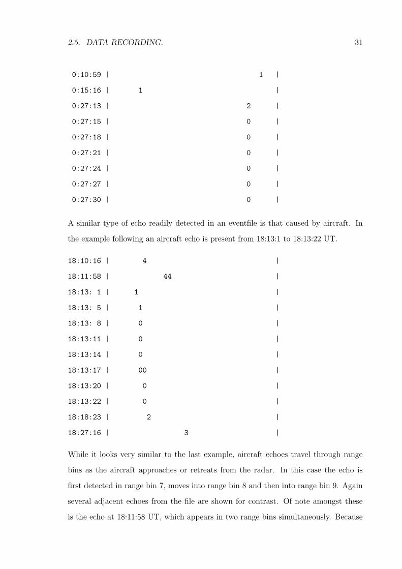
2.5. DATA RECORDING. 31
0:10:59 | 1 |
0:15:16 | 1 |
0:27:13 | 2 |
0:27:15 | 0 |
0:27:18 | 0 |
0:27:21 | 0 |
0:27:24 | 0 |
0:27:27 | 0 |
0:27:30 | 0 |
A similar type of echo readily detected in an eventfile is that caused by aircraft. In
the example following an aircraft echo is present from 18:13:1 to 18:13:22 UT.
18:10:16 | 4 |
18:11:58 | 44 |
18:13: 1 | 1 |
18:13: 5 | 1 |
18:13: 8 | 0 |
18:13:11 | 0 |
18:13:14 | 0 |
18:13:17 | 00 |
18:13:20 | 0 |
18:13:22 | 0 |
18:18:23 | 2 |
18:27:16 | 3 |
While it looks very similar to the last example, aircraft echoes travel through range
bins as the aircraft approaches or retreats from the radar. In this case the echo is
first detected in range bin 7, moves into range bin 8 and then into range bin 9. Again
several adjacent echoes from the file are shown for contrast. Of note amongst these
is the echo at 18:11:58 UT, which appears in two range bins simultaneously. Because
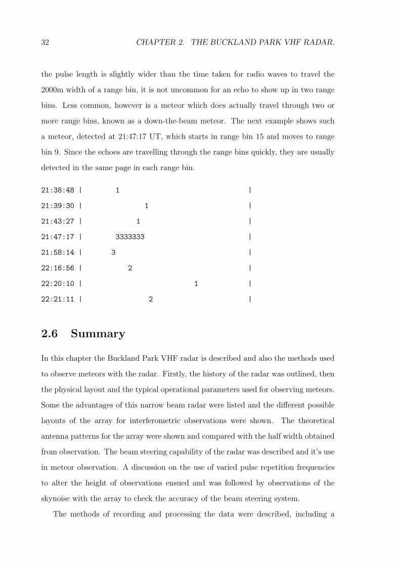
32 CHAPTER 2. THE BUCKLAND PARK VHF RADAR.
the pulse length is slightly wider than the time taken for radio waves to travel the
2000m width of a range bin, it is not uncommon for an echo to show up in two range
bins. Less common, however is a meteor which does actually travel through two or
more range bins, known as a down-the-beam meteor. The next example shows such
a meteor, detected at 21:47:17 UT, which starts in range bin 15 and moves to range
bin 9. Since the echoes are travelling through the range bins quickly, they are usually
detected in the same page in each range bin.
21:38:48 | 1 |
21:39:30 | 1 |
21:43:27 | 1 |
21:47:17 | 3333333 |
21:58:14 | 3 |
22:16:56 | 2 |
22:20:10 | 1 |
22:21:11 | 2 |
2.6 Summary
In this chapter the Buckland Park VHF radar is described and also the methods used
to observe meteors with the radar. Firstly, the history of the radar was outlined, then
the physical layout and the typical operational parameters used for observing meteors.
Some the advantages of this narrow beam radar were listed and the different possible
layouts of the array for interferometric observations were shown. The theoretical
antenna patterns for the array were shown and compared with the half width obtained
from observation. The beam steering capability of the radar was described and it’s use
in meteor observation. A discussion on the use of varied pulse repetition frequencies
to alter the height of observations ensued and was followed by observations of the
skynoise with the array to check the accuracy of the beam steering system.
The methods of recording and processing the data were described, including a

2.6. SUMMARY 33
discussion on detection algorithms, required to discriminate between the meteor echoes
and noise, reducing the volume of data recorded without missing meteor echoes, all
done in real time. Lastly, examples of the “eventfiles” produced by the system were
given to illustrate their use in giving a summary of the data recorded.

34 CHAPTER 2. THE BUCKLAND PARK VHF RADAR.

Chapter 3
Radio meteor theory
This chapter is concerned with fundamental meteor theory and how it relates to ob-
serving meteors with radar. First, we deal with ablation theory, in which the ionisation
profile of meteors is modelled. Next, the effects of fragmentation, thermal conduction
and heat capacity of the meteoroid on the ablation process are outlined. Diffusion of
the ionisation and the effect on it of the Earth’s magnetic field is added to the model.
The Fresnel theory of radio backscatter is covered, and then a discussion of attenua-
tion factors including the effects of Faraday rotation. The radar response function is
covered in the later sections.
3.1 Ablation
Early work on the classical theory of atmospheric ablation assumed that meteoroids
had a compact single body stony structure. Much of this work was done by Opik
(1937) (Opik 1958) and Whipple (1938) (Whipple 1943). McKinley (1961) notes that
observations do not follow the rules for solid bodies, but are more suited to a theory
derived for porous or crumbly objects. Jacchia (1955) put forward a dustball model in
which the meteoroid was composed of many small grains. Ceplecha et al. (1998) note
that a double biased selection by Verniani (1965) of Super-Schmidt meteors brought
about an impression that all meteoroids are made up of low density crumbly or friable
35

36 CHAPTER 3. RADIO METEOR THEORY
material. This came about because Verniani used a selection of “best” meteors from
the meteors which Jacchia & Whipple (1961) had analysed. These meteors were
themselves a selection from the meteors published by McCrosky & Posen (1961). The
effect of the two sets of selections was to retain only those meteors which showed
the characteristics of low density particles. A quantitative model was put forward by
Hawkes & Jones (1975), assuming that the meteoroids are a conglomerate of silicate
and metallic oxide grains bonded with a material, possibly organic in nature, with
a much lower boiling point. Fisher et al. (2000) suggest that ablation of particles
first heats and boils off this “glue” component, releasing the silicate and metallic
oxide grains, which then heat to their boiling point and vaporise producing light and
ionisation by collision with air molecules.
3.1.1 Preheating, ablation and the equations of motion
As the particle enters the atmosphere the rate of change of its height, z, can be given
as:
dz
dt= −v cosχ(t) (3.1)
where v is the meteoroid speed and χ(t) is the zenith angle which, since the earth is not
flat, changes with time, t. We ignore the effect of gravity, since this is not significant
for zenith angles less than 85. The shape, mass, and density of the particle are all
unknowns, and thus we define a dimensionless shape factor, A, such that A(m/ρm)2/3
is the effective cross sectional area of the body, where m is the mass and ρm is the
effective density of the meteoroid. For a sphere, A = (9π/16)1/3 ≈ 1.21. It is expected
that irregular bodies will have a value of A of the same order due to rotation. In a
time dt, the mass of air intercepted by the body is:
dma = A
(
m
ρm
)2/3
ρavdt
where ρa is the air density. For the small meteoroids that generate the ionisation
detected by radar the dimensions of the meteoroid are much smaller than the mean
free path at these heights. Thus we would expect that the interaction between the

3.1. ABLATION 37
atmosphere and the meteoroid to be of a molecular nature. For larger meteoroids,
(Brown et al. 1994) we would need to consider fluid flows and “air caps”, when a
layer of air molecules bouncing off the meteoroid shields the meteoroid against the
atmosphere.
Even though the meteoroid meets several times it’s own mass in air molecules
during it’s passage through the atmosphere, and with sufficient speed to embed the
molecules several atomic layers deep in the meteoroid, the lack of any observable
nitrogen in collected micrometeorites is evidence that there is no appreciable accretion
of atmospheric gases during flight (Flynn 1989). Thus, the air molecules are assumed
to donate their momentum and energy, but not mass, to the meteoroid. These particles
will give up momentum at the rate of:
Γvdma
dt= ΓA
(
m
ρm
2/3)
ρav2 units of momentum per second (3.2)
where Γ is the drag coefficient, and has a value from 0.5 to 1.0. Since the meteoroid
is losing momentum at a rate of mdv/dt units per second, we can equate the two to
give the drag equation.
dv
dt= − ΓA
m1/3ρ2/3m
ρav2 (3.3)
By the principle of conservation of energy, we assume that the kinetic energy
“lost” by the air molecules is used for heating and producing small amounts of light
and ionisation. Since the meteoroid intercepts a mass dma in a time dt, the kinetic
energy lost by the air molecules is:
dEKE = −1
2dmav
2 = −A2
(
m
ρm
) 23
ρav3dt (3.4)
For the period before the onset of ablation, the heat loss due to evaporation is
small, and thermal re-radiation is the main loss. As the temperature rises evaporation
becomes more significant. The evaporation of material from the heated surface of a
meteoroid at a temperature T is assumed to be described by the Langmuir expression
for evaporation into a vacuum. The evaporation rate per unit area, G, is given by:
G = ψpν√M√
2πRT(3.5)

38 CHAPTER 3. RADIO METEOR THEORY
where pν is the vapour pressure of the evaporated material, M is the molecular weight
of the vapour and R is the gas constant. The coefficient of condensation, ψ has the
value of 1.0 for metals and is smaller for other materials. Bronshten (1983) suggests
using 0.5. The inclusion of this factor has a very minor effect on theoretical ablation
profiles and it has therefore been set to unity (Elford - private communication). A
typical value of M is 0.045 (Love & Brownlee 1991). The rate of change of the vapour
pressure is related to the latent heat of vaporisation, l by the Clausius - Clapeyron
relation:
d ln pνdT
=l
RT 2
This integrates to:
ln pν = −l
RT+ C (3.6)
Most workers on meteor ablation express the vapour pressure dependence on temper-
ature as:
log10 pν = C1 +C2
T(3.7)
where pν is in pascals and C1 and C2 are listed as constants of the ablating material.
Typical values for the constants for stony materials are C1 = 12.5 and C2 = −21000
(Bronshten 1983).
The mass loss due to ablation, ignoring the effects of spallation or thermionic
emission (Sorasio et al. 2001), is given by the differential mass equation,
dm
dt= −A
(
m
ρm
) 23
G
= −A(
m
ρm
) 23
10C110C2T
√
M
2πRT
= −A(
m
ρm
) 23 K1e
K2T
√T
(3.8)
where K1 and K2 are constants of the meteoroid material (Lebedinets et al. 1973).
Thus the rate of change of the surface temperature of the meteoroid, T is given by
the heating equation,
dT
dt=
A
cm1/3ρ2/3m
(
Λρav3
2− 4σε(T 4 − T 4
a )−LK1e
K2T
√T
)
(3.9)

3.1. ABLATION 39
Where c is the specific heat of the meteoroid material, Λ is the heat transfer coefficient,
σ is the Stefan-Boltzmann constant, ε is the emissivity of the meteoroid, Ta is the
ambient temperature and L is the sum of the latent heats of fusion and vaporisation
of the meteoroid material. We assume that the meteoroid is small enough to be
isothermal at all times (< 0.1 mm radius). An examination of the properties of the
emissivity of small spherical particles (Greenberg 1978) shows that ε is a function
of the particle size and temperature. For meteoroid masses exceeding 10−11 kg and
temperatures exceeding 400 K the value of ε can be set to one.
In ablation studies, the exact value of the ambient temperature, Ta has become
more significant with the introduction of theories on materials with low ablation tem-
peratures. At 1 A.U. from the sun, the equilibrium temperature of a meteoroid is 279
K. As a particle approaches the sunlit side of the Earth, the received solar radiation
flux is increased because of reflection from the Earth, increasing the equilibrium tem-
perature of a meteoroid with an emissivity of one from 279 K to ∼ 307 K. However,
unless the particle is very small (< 10µm radius ) there is not enough time spent close
to the Earth to increase the meteoroid’s free space temperature significantly. While
the atmospheric temperature between 100 and 200 km rises from 200 to 1000 K, and
slower meteoroids may spend several seconds in this region, satellite measurements of
the radiance from above 100 km show that it is equivalent to that of a black body at
∼ 280K with gaps due to absorption from water, carbon dioxide and ozone. Thus the
value of Ta can be set to 280 K for all meteoroids at all heights.
The heat transfer coefficient usually lies between 0.1 and 0.6 (McKinley 1961) and
the sum of the latent heats of fusion and vaporisation has been taken as 6.0×10⁶J kg−1
by Nicol et al. (1985) in their modelling of ablation. The sum of the latent heats of
fusion and vaporisation is dominated by the latent heat of vaporisation. We note that
this means the total latent heat can be found from equation 3.7.
When the ablated atoms collide with air particles, some interactions produce free
electrons. If β is the probability that a single ablated atom of mass µ produces a free
electron on collision, and q is the number of electrons produced per unit path length
40 CHAPTER 3. RADIO METEOR THEORY
then in time dt,
qv dt = −βµdm (3.10)
The value of β depends on the speed of the meteoroid and the material of the
meteoroid and can be greater than one as an atom may undergo several collisions.
Jones (1997) has produced a theoretical derivation of the value of β that can be
applied to faint radio meteors with speeds ≤ 35km s−1; it can be approximated by:
β ' 9.4× 10⁻⁶(v − 10)2v0.8 (3.11)
For visual meteors with speeds in the range 30 to 60km s−1, Jones approximates
simulation results with:
β = 4.91× 10⁻⁶v2.25 (3.12)
Substituting equation 3.8 into equation 3.10 and rearranging we obtain the ionisa-
tion equation:
q =βA
µv
(
m
ρm
) 23 K1e
K2T
√T
(3.13)
A simpler set of equations could be obtained by assuming no mass loss until the
surface of the meteoroid reaches the “boiling point” of the material, defined as the
temperature at which the vapour pressure is equal to the local atmospheric pressure,
but usually refers to the value at sea level.
In this simpler model, the meteoroid is assumed to begin ablating at this “boiling
point” and remain at this temperature. During ablation the rate of change of temper-
ature would equal zero and the mass loss term in the heating equation would equal
the sum of the other two terms, giving mass loss and ionisation equations which con-
tain the energy gain term and the radiative term. However, the concept of a boiling
point has little meaning in the case of a meteoroid which is experiencing only a small
percentage of the air pressure at sea level. Numerical solutions of the heating and
deceleration equations for different types of materials has shown that meteoroids do
not reach the “boiling point” of the material during flight (Elford 1999), and there is
substantial evaporation even before the particle can be said to be “boiling”. Thus the
“simple model” is a poor approximation to the ablation of meteoroids.
3.1. ABLATION 41
The problem of solving the differential equations of motion and ablation has been
attacked from many angles. Whipple (1938) used Hoppe’s solution (Hoppe 1937)
which was the first closed mathematical solution to the equations of motion and ab-
lation with constant coefficients. Bronshten (1983) presented a more general solution
with changing coefficients. These analytical solutions have become less important with
the advent of powerful numerical models of meteoroid heating and ablation. A com-
prehensive analysis, applicable to large bodies (those which become meteorites) was
performed by Pecina & Ceplecha (1983) (Pecina & Ceplecha 1984) and is summarised
by Ceplecha et al. (1998) (see Section 3.1.3. An analysis appropriate to smaller bodies
is given by Love & Brownlee (1991).
3.1.2 The effects of meteoroid radius on ablation
The ablation theory described in the previous section doesn’t fully take into account
the effects of heat capacity and thermal conduction of the meteoroid material on the
preheating and ablation processes.
During preheating the kinetic energy given up by the air molecules goes into heating
the meteoroid and some of this is re-radiated. For particles above a certain size, the
effect of heat transfer through the body is significant, and we can rewrite equation 3.9
in terms of the body radius r and mean body temperature Tm.
dTmdt
=12Λρav
3 − 4εσ(T 4 − T 4a )
43rρmc
(3.14)
The mean temperature of a meteoroid of radius r is
Tm =3
r3
∫ r
0
R2 T (R) dR
The relationship between the instantaneous surface temperature and the mean
temperature depends on the radius and thermal conductivity of the meteoroid, and
the total history of the surface heating of the meteoroid (Elford 1999).
Equation 3.14 can be used to investigate the height of commencement of ablation
for various meteoroid compositions, speeds, and sizes (Jones & Kaiser 1966). Jones

42 CHAPTER 3. RADIO METEOR THEORY
Figure 3.1: Theoretical beginning height of ablation for single stony meteoroids en-tering the atmosphere at a zenith angle of 45, shown as a function of mass (after(Ceplecha et al. 1998)) See text for details
and Kaiser identify three critical values for the meteoroid radius, depending on speed,
which are R1, R2 and R3, as shown in Figure 3.1, which shows theoretical beginning
heights of ablation for single stony meteoroids entering the atmosphere at a zenith
angle of 45, shown as a function of mass. The values are calculated for the CIRA-
86 atmosphere, June 45 N, except for the dotted curve for 11km/s which applies in
December.
For meteoroids with a radius less than R2, the effect of thermal capacity can be

3.1. ABLATION 43
neglected, and the heating process is dominated by re-radiation. This delays the com-
mencement of ablation due to heat loss. When the radius is smaller still, deceleration
becomes significant and delays ablation further due to the reduction in speed. R1 is
defined such that for radii less than R1 the meteoroid does not begin to ablate; this
is the micrometeoroid limit. The majority of meteors observed by the Buckland Park
VHF radar are caused by meteoroids with radii lying on the flat region of the curves
in Figure 3.1 between R1 and R2.
For radii between R2 and R3, the thermal capacity effect is much greater than
the radiative effect. In this case, the onset of ablation is delayed due to the finite
heat capacity of the meteoroid. A radius greater than R3 means that a meteoroid will
develop a thermal gradient which can lead to fragmentation due to heat stresses (Elford
1999). It has been observed that the majority of +10 magnitude and brighter radio
meteors (meteoroids larger than R2 in radius) don’t begin ablation at the theoretical
heights shown as the dashed lines in Figure 3.1, but instead behave more like smaller
meteoroids. Hawkes & Jones (1975) attribute this behaviour to fragmentation of a
“dust ball” or conglomerate type of meteoroid.
Not only does the inclusion of heat capacity and radiation delay the commencement
of ablation, but also it causes the height of maximum ionisation to be reduced and
the value of the maximum to be increased. Hughes (1978) gives a correction to the
classical ablation theory; where ρa(max) is the density of the atmosphere at the height
of maximum ionisation, then the density of the atmosphere at the new height is given
by:
ρa(max)′ = ρa(max)(1 +γ
3)
where γ is defined by:
γ = c(Tb − Ta)
L
where Tb is the boiling point of the material. The maximum ionisation is larger by a
factor of (1 + γ/3)3.

44 CHAPTER 3. RADIO METEOR THEORY
3.1.3 The effects of fragmentation on ablation
Many researchers have noted that many optically observed meteors, behave differently
to predictions based on ablation theory (Jacchia et al. 1950, Cook 1954, Jacchia 1955,
Whipple 1955). The first evidence came from the observed “flaring” near the end of
some meteor trails, that meteor trails are shorter than expected and that instantaneous
light production from an extended area behind the body of the meteoroid, known as
“meteor wakes”, can be detected (Hawkes & Jones 1975, Verniani 1969). Several
studies of faint meteors (Campbell et al. 1999, Fleming et al. 1993) have found that
meteor light curves are skewed toward the beginning of the trajectory. LeBlanc et al.
(2000) have presented evidence for transverse separation of meteoroid fragments in an
image of a meteor taken from an aircraft observing the 1998 Leonids Meteor shower
with an intensified CCD camera.
Two main types of fragmentation have been identified by Babadzhanov (1993)
and Ceplecha (1993); quasi-continuous and gross fragmentation. Quasi-continuous
fragmentation, or spallation occurs when small parts of the meteoroid are gradually
broken off or ejected during ablation, and subsequently ablate individually. Gross
fragmentation occurs when the meteoroid breaks up into two or more pieces which
are roughly the same size, which may then fragment further. In addition to these
two fragmentation processes, Hawkes and Jones have described a “dustball” model
(Hawkes & Jones 1975), where the meteoroid entering the atmosphere is made up of a
loosely bonded conglomerate of silicate and metallic oxide grains. In this model, the
“glue” which bonds the grains is assumed to have a much lower boiling point than
the grains, and thus is evaporated during preheating, leaving a cloud of similar size
particles as in a shotgun blast.
Pecina & Ceplecha (1983) (Pecina & Ceplecha 1984) have produced a solution
to their differential equations of motion, by writing them in terms of l = l(t), ie
the distance l travelled by the body in its trajectory. The problem of keeping the
coefficients of the differential equations constant is overcome by the means of applying

3.1. ABLATION 45
it to small intervals of time after ReVelle (1979). This solution ignores the effects
of radiation on ablation ie it omits the 4σε(T 4 − T 4a ) term from Equation 3.9 and
thus is not applicable to particles smaller than 1 mm (Ceplecha et al. 1998). It is
capable of not only accounting for continuous fragmentation but also incidences of
gross fragmentation at discrete trajectory points (Ceplecha et al. 1993).
Fisher et al. (2000) have used a numerical integration of the equations of motion
and ablation to model the flight of meteors composed of multiple grains of different
sizes, assuming that they are held together by a “glue” which boils off at a lower
temperature than the ablation of the grains. Thus the grains separate and can be
individually modelled. Fisher et al calculated the lag between these grains, expressing
it by the following:
lag =∑
(vl − vs)dt
Where vl represents the velocity of the largest grain in the group and vs is the velocity
of the smallest.
Fisher et al have performed this modelling in order to predict the effect of frag-
mentation on television observations of wake, trying to determine if the lag is visible
and at what height the separation of the grain is taking place. They therefore mod-
elled extreme differences in the grain sizes (diameters an order of magnitude different),
although the work of Simonenko (1968) and Campbell et al. (1999) indicate that the
range of masses of the grains is quite narrow. Elford & Campbell (2001) have per-
formed a similar numerical integration model of fragmentation, and the consequences
for radar observations of fragmenting meteors. The effects of fragmentation on radar
echoes can be treated by looking at two limiting cases: (a) where the fragments be-
come separated in a direction parallel to the motion of the meteoroid; and (b) where
the separation is orthogonal to the motion of the meteoroid. The first can be caused
by the differential deceleration of different size and shape particles, but for the second
there would have to be some mechanism to give the bodies an orthogonal velocity.
This could be due to rotation of the body before fragmentation or due to the gas
pressure of boiling “glue” type substances. The effects of fragmentation are discussed

46 CHAPTER 3. RADIO METEOR THEORY
in more detail later in the chapter and in chapter 5, but type (a) will give separate
radar reflections which could interfere with each other, and type (b)will produce a
broadening of the ionised column.
3.2 Formation of the ionised trail and initial radius
As the meteoroid travels through the atmosphere it leaves a trail of ablated atoms,
molecules and ionisation behind as described by equation 3.13. The majority of meteor
trails detected by radar are produced by meteoroids of mass smaller than 10−5kg and
ablation studies show that such trails extend over a height range of about 10km. For
radar studies, the ionisation distribution can be considered as a parabolic function of
the density of the atmosphere about the height of maximum ionisation. The maximum
value of the line density of the ionisation (in electrons per metre) is proportional to
the initial mass of the meteoroid and to cos z where z is the zenith angle of the trail.
The ablated atoms coming off the meteoroid are still travelling with most of the
speed of the meteoroid and would require several collisions to slow them down to
thermal velocities (Opik 1955). This process takes of the order of a millisecond at
100km (Massey & Sida 1955) and produces an ionised column of Gaussian cross-
section and initial radius r0. Estimates of the initial radius have been made both
theoretically and experimentally, and depend on β the probability that a single ablated
atom produces a free electron on collision. Bronshten (1983) indicates that the initial
radius can be expressed as:
r0 = ρaavb
where a ∼ −1 and b ∼ 0.8. However Opik (1958) suggested that continuous fragmenta-
tion of rotating dustball type meteoroids will produce a lateral spread of the ablating
particles and thus increase the initial radius. Radio measurements of meteors with
magnitudes between +5 and +10 show an initial radius (assuming a Gaussian distri-
bution) where a lies between -0.25 and -0.45, while brighter meteors (Magnitude +2.5)
show a much more rapid height variation (Baggaley 1970, Baggaley & Fisher 1980).
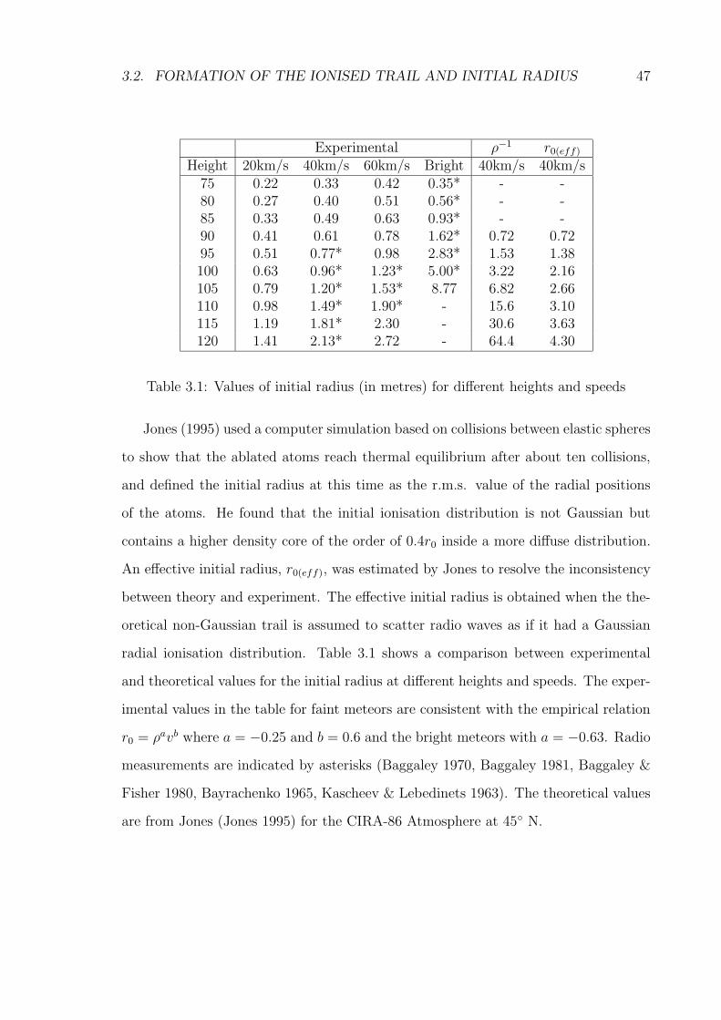
3.2. FORMATION OF THE IONISED TRAIL AND INITIAL RADIUS 47
Experimental ρ−1 r0(eff)
Height 20km/s 40km/s 60km/s Bright 40km/s 40km/s75 0.22 0.33 0.42 0.35* - -80 0.27 0.40 0.51 0.56* - -85 0.33 0.49 0.63 0.93* - -90 0.41 0.61 0.78 1.62* 0.72 0.7295 0.51 0.77* 0.98 2.83* 1.53 1.38100 0.63 0.96* 1.23* 5.00* 3.22 2.16105 0.79 1.20* 1.53* 8.77 6.82 2.66110 0.98 1.49* 1.90* - 15.6 3.10115 1.19 1.81* 2.30 - 30.6 3.63120 1.41 2.13* 2.72 - 64.4 4.30
Table 3.1: Values of initial radius (in metres) for different heights and speeds
Jones (1995) used a computer simulation based on collisions between elastic spheres
to show that the ablated atoms reach thermal equilibrium after about ten collisions,
and defined the initial radius at this time as the r.m.s. value of the radial positions
of the atoms. He found that the initial ionisation distribution is not Gaussian but
contains a higher density core of the order of 0.4r0 inside a more diffuse distribution.
An effective initial radius, r0(eff), was estimated by Jones to resolve the inconsistency
between theory and experiment. The effective initial radius is obtained when the the-
oretical non-Gaussian trail is assumed to scatter radio waves as if it had a Gaussian
radial ionisation distribution. Table 3.1 shows a comparison between experimental
and theoretical values for the initial radius at different heights and speeds. The exper-
imental values in the table for faint meteors are consistent with the empirical relation
r0 = ρavb where a = −0.25 and b = 0.6 and the bright meteors with a = −0.63. Radio
measurements are indicated by asterisks (Baggaley 1970, Baggaley 1981, Baggaley &
Fisher 1980, Bayrachenko 1965, Kascheev & Lebedinets 1963). The theoretical values
are from Jones (Jones 1995) for the CIRA-86 Atmosphere at 45 N.
48 CHAPTER 3. RADIO METEOR THEORY
3.3 Radio wave scattering from meteor trails
3.3.1 Underdense and overdense trails
The radio reflection coefficient of a section of the ionised column depends on the volume
density of the electrons. The radio wave penetrates the plasma essentially unchanged if
secondary scatter is insignificant, and the total scattered radiation is simply the sum
of the contributions of individual electrons. This condition defines the underdense
meteor trail, and applies to trails with an electron line density < 1014 electrons per
metre. If the electron density is increased, say above 1015 electrons per metre, then
the secondary scattering becomes significant and the dielectric constant of the plasma
becomes negative. This is known as an “overdense” trail and the wave disturbance
within the trail has become evanescent. An overdense trail can be modelled as a
metallic cylinder which expands as the trail diffuses and suddenly collapses when the
electron concentration falls below the critical value.
3.3.2 Transverse and down beam echoes
Before introducing the theory of radio back-scatter from meteor trails in detail, some
of the geometry of meteor trails to radar observation must be discussed. The direction
of arrival to a ground based observer of a meteoroid is determined by the combination
of the meteoroid’s orbit, and the orbit and rotation of the Earth. The angle between
this direction and the beam direction has a great effect on the strength of the radar
echo, and means that only two main groups of meteors need to be considered. The
geometry of these groups is shown in Figure 3.2. The first is the “down the beam”
echo, which was first observed by Hey & Stewart (1947). This type of echo is analogous
to detecting aircraft with airport radar. It occurs when a meteoroid produces a large
amount of ionisation and reflection of the radio waves occurs from the “head” of the
meteor, the position where the meteoroid is producing the ionisation. The radio waves
are considered to be reflecting from an overdense region of ionisation surrounding the

3.3. RADIO WAVE SCATTERING FROM METEOR TRAILS 49
Radar
Meteoroid path
Radar Beam
(a)
Radar
Radar Beam
Meteoroid Path
(b)
Figure 3.2: Geometry of the two types of meteor echoes. (a) shows a “down the beam”echo and (b) shows a “transverse” or specular echo
ablating meteoroid. The echo shows up in a number of range bins, depending on the
angle to the radar beam, and the width of the radar beam. For a narrow beam radar
like the Buckland Park VHF radar, the direction of arrival must be quite close to the
radar beam direction to appear in many range bins, ie the meteoroid must be coming
“down the beam”, hence the naming of this type of echo. This type of echo is relatively
infrequent, since there must be enough ionisation forming instantly at the head of the
meteor trail to form an overdense region of sufficient size to produce a detectable radar
return, and the range of allowed angles of arrival which will give echoes in multiple
range bins is small.
The second type of echo is the “transverse” echo, which occurs when the trail of
the meteor is orthogonal to the radar beam. This type of echo is much more common
than the “down the beam” echo, as coherent reflection occurs from a relatively large
length of trail near the orthogonal point, and thus smaller ionisation densities can be
detected. This type of echo is discussed in detail in the next section.

50 CHAPTER 3. RADIO METEOR THEORY
3.3.3 The basic Fresnel theory of radar back-scatter from me-
teor trails
Consider the idealised case of a meteor trail where the diameter of the trail is much
smaller than the wavelength and the effects of diffusion are ignored. We also assume
that the trail is underdense, so secondary radiative and absorptive effects can be
neglected, and we assume the effects of the geomagnetic field can be neglected. The
power flux of the incident wave at a point on the trail in watts per m2 is given by:
Φi =PTGT
4πR2(3.15)
where PT is the transmitted power, GT is the antenna gain relative to an isotropic
radiator and R is the distance from the point to the radio transmitter. The scattering
cross section of a free electron is:
σe = 4πr2e sin
2 γ (3.16)
where re is the classical electron radius and γ is the angle between the electric vector
of the incident wave and the line of sight of the receiver. For the case of back-scatter,
γ = π/2 and σe = 1.0 × 10⁻²⁸ m2. Thus the power flux of radiation back-scattered
from a single electron to the receiving antenna is:
Φe = Φiσe
4πR2= Φi
(reR
)2
(3.17)
Consider a small region of the trail ds. If q is the electron line density of the trail and
Z0 is the wave impedance of free space, then since the trail diameter is assumed to
be small compared to the wavelength, the electrons in ds can be assumed to scatter
in phase, and the maximum possible amplitude of the returned electric field, E0, from
the segment of trail is given by:
E0 = q√
2Z0Φe ds (3.18)
The returned wave has travelled a distance 2R, and therefore has a modulation factor
of exp(j(ωt− 2kR)), where k = 2π/λ. The amplitude ER, of the field at the receiving

3.3. RADIO WAVE SCATTERING FROM METEOR TRAILS 51
antenna due to scattering from the whole trail is:
ER = q√
2Z0Φe
∫
exp(
j(ωt− 2kR))
ds (3.19)
where the integral is taken over the length of the trail and the assumption has been
made that q is constant.
The integral may be simplified by using the approximation R ≈ R0 + s2/(2R0)
where s is the distance along the trail from ds to the orthogonal point ( “t0 point”),
whose range is R0. For a trail length of 10km, and R0 = 100km the error is about
0.001%. Using the transformation x = 2s/√R0λ, we obtain:
ER =
√
R0λ
42Z0Φe exp
(
j(ωt− 2kR0))
q
∫
exp(
j(−πx2/2))
dx,
ER =
√
R0λ
42Z0Φe exp
(
j(ωt− 2kR0))
q(C − jS) (3.20)
where C and S are the Fresnel integrals of diffraction theory:
C =
∫
cos
(
πx2
2
)
dx, and (3.21)
S =
∫
sin
(
πx2
2
)
dx (3.22)
In Figure 3.3, C and S have been plotted orthogonally resulting in the Cornu spiral.
Note that the spiral is oriented differently to how many optics textbooks show it,
as optics and radio physics use different conventions for defining the phase in the
exponential notation. The origin of the meteor echo is held at the centre of the upper
spiral, at x = −∞. The normalised variable, x is often referred to as the Fresnel
length. As the electric field phasor traces out the upper spiral, the amplitude increases
continuously and the phase angle decreases. The amplitude reaches its maximum value
at x = +1.21 as the meteor crosses the first fresnel zone past the t0 point (x = 0).
The phase reaches a minimum value at x = +0.6. Past these points the amplitude
and phase oscillate with decreasing magnitude and increasing frequency, as the electric
field phasor traces out the lower spiral. The amplitude and phase oscillations are in
quadrature, with the phase leading.
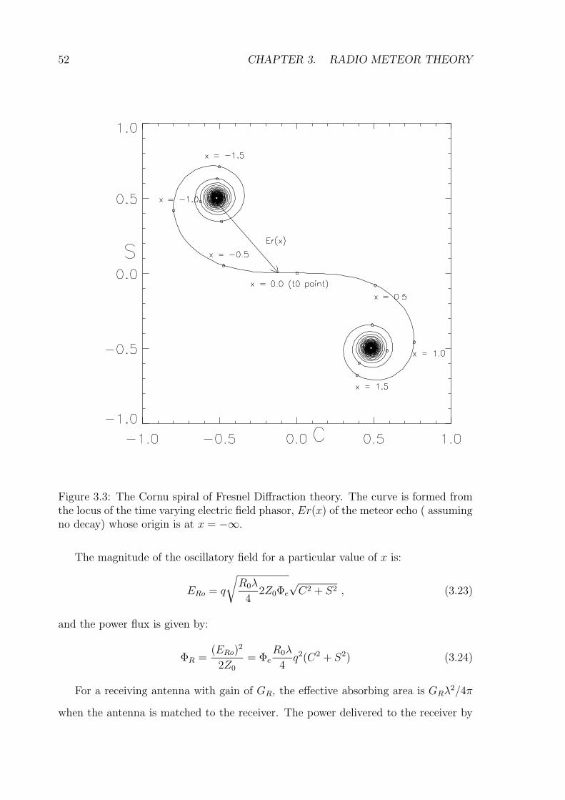
52 CHAPTER 3. RADIO METEOR THEORY
Figure 3.3: The Cornu spiral of Fresnel Diffraction theory. The curve is formed fromthe locus of the time varying electric field phasor, Er(x) of the meteor echo ( assumingno decay) whose origin is at x = −∞.
The magnitude of the oscillatory field for a particular value of x is:
ERo = q
√
R0λ
42Z0Φe
√C2 + S2 , (3.23)
and the power flux is given by:
ΦR =(ERo)
2
2Z0
= ΦeR0λ
4q2(C2 + S2) (3.24)
For a receiving antenna with gain of GR, the effective absorbing area is GRλ2/4π
when the antenna is matched to the receiver. The power delivered to the receiver by

3.4. DIFFUSION OF THE IONISATION 53
scattering from the whole trail is:
PR =ΦeGRλ
3R0
16πq2(C2 + S2) =
ΦiGRλ3
16πR0
q2r2e(C
2 + S2), (3.25)
Substituting for Φi, this received power is:
PR = PTGTGRλ3q2r2
e
C2 + S2
64π2R30
(3.26)
While the trail is being formed the value of C2+S2 increases steadily as the meteoroid
approaches the t0 point and then oscillates. Figure 3.4 (Curve A) shows the returned
echo power and the phase. Note the oscillations after the t0 point which are present
in both the phase and the amplitude of the echo, and are analogous to optical Fresnel
diffraction at a straight edge. Curves B to D show the effects of diffusion, which is
discussed in Section 3.4.
Elford & Campbell (2001) have shown that the effect of fragmentation is to pro-
gressively “wash out” the post-t0 oscillations, depending on the separation and number
of the fragmented particles. This is due to type (a) fragmentation (see Section 3.1.3,
where the particles are separated in a direction parallel to the motion of the meteoroid.
Each of the trails associated with the particles produces an electric field phasor which
have different values for x at any given time. The returned signal is the sum of the
phasors which will tend to “wash out” the observed oscillations as they interfere with
each other. The effect will be greater for greater extension of the bunch of particles
along the path. There is also an effect in the pre-t0 phase, and this is discussed in
chapter 5.
3.4 Diffusion of the ionisation and the effect of the
Earth’s magnetic field
Once the trail is formed, it will expand rapidly due to ambipolar diffusion, atmospheric
turbulence and loss of ionisation through recombination and ionic reactions. Also the
whole trail will be affected by large-scale wind shears which will bend and twist the

54 CHAPTER 3. RADIO METEOR THEORY
Figure 3.4: Returned echo power (a) and phase (b). Curve A shows no diffusion, andcurves B to D show the effects of increasingly severe diffusion.
ionisation column. Radio studies have shown that the most important dissipation
factor is ambipolar diffusion, which reduces the volume density but does not affect
the line density. At heights below 90 km, where the effect of the Earth’s magnetic
field on the diffusing ionisation may be ignored, the volume density of electrons (and
ions) at time t and distance r from the column axis is described by the radial diffusion
equation,
δn(r)
δt= D∇2n(r) (3.27)
3.4. DIFFUSION OF THE IONISATION 55
where D is the ambipolar diffusion coefficient in square metres per second and n(r) is
the volume density of the ionisation. For a cylindrical column of ionisation with initial
radius r0, Jones (1995) has shown that, when 4Dt À r20, the appropriate solution of
this equation is:
n(r, t) =q
πa2exp
(
−r2
a2
)
(3.28)
where q is the electron line density and a2 = 4Dt+r20. Jones pointed out that 4DtÀ r2
0
may not always be satisfied when t is small.
The ambipolar diffusion coefficient for electrons in a meteor trail (ignoring the
geomagnetic field) is given by:
D = Di(1 +TeTi
) (3.29)
where Di is the diffusion coefficient for the positive ions and Te and Ti are the electron
and ion temperatures respectively (Mason & Daniel 1988).
The plasma column must be in a condition of charge neutrality at all times and
so the radial distribution of the electrons will be the same as that of the thermalised
ion, but the electrons will cool much slower than the ions, and can remain hot for
times ranging from of the order of 1 ms at 80 km to ∼ 150ms at 115 km as shown
in Table 3.2 (Baggaley & Webb 1977). The presence of “hot” electrons will increase
the rate of diffusion of the ionisation during the early evolution of the trail. Trails
with line densities less than 2.5 × 10¹⁴m−1 remain “hot” at 110 km for over 80 ms
after the trail has been formed. After 25 ms, the “electron temperature” is still about
600K or 2.5 times the ambient value. This increases the coefficient of diffusion of the
trail by ∼ 75%. After the early stages of formation of the meteor trail, the ions and
electrons can be considered to be in thermal equilibrium with the ambient atmosphere
for meteor heights below 95 km, so that Te = Ti and D = 2Di. The diffusion coefficient
can be described in terms of the zero field mobility K of a group of ions, using the
Einstein relation:
Di = kTiK
e(3.30)

56 CHAPTER 3. RADIO METEOR THEORY
Height Line Density (m−1)km < 2.5× 10¹⁴ 2.5× 10¹⁵ 2.5× 10¹⁶
80 0.6 0.6 0.590 4.0 3.3 1.8100 21 16 7.5110 85 66 45120 240 240 240
Table 3.2: Thermalisation times for electrons(ms) (time to reach 110 % of ambienttemperature)
where k is Boltzmann’s constant and e is the electronic charge. Laboratory measure-
ment of K allow the diffusion coefficients to be calculated. In the case of alkali ions
in nitrogen, D ≈ 1.4 × 10⁻⁵T 2p−1, where T is the ambient gas temperature and p is
the gas pressure.
For meteor trails at heights above 90 km, the effect of the Earth’s magnetic field
must be taken into account when considering the diffusion of the ionisation. The
diffusion coefficients have different values in the directions parallel and orthogonal to
the magnetic field, and this causes the ionisation to diffuse anisotropically, notably
much slower orthogonal to the field, thus giving our diffusing cylinder of ionisation an
elliptical cross-section, and when the effect is stronger, producing a sheet of ionisation.
This problem was considered by Kaiser et al. (1969), and Jones (1991), who derived
expressions for the diffusion coefficients in two directions, and their dependence on
height and the angle between the trail and the field. Elford & Elford (1999) looked at
Jones’ expressions and applied published values of momentum transfer cross-section
data for electron collisions with atmospheric gases to estimate values of the diffusion
coefficients orthogonal to the field. Their work brought the problem to the attention
of Robson (2001), a plasma physicist, who noted that no one had previously put the
meteor problem in the context of mainstream plasma physics. The following is a
summary of the outcomes of Robson’s analysis.
Considering a meteor trail oriented at an arbitrary angle θ to the geomagnetic field,
B, the radar sends a signal with wave number ko to the trail, where it is scattered.
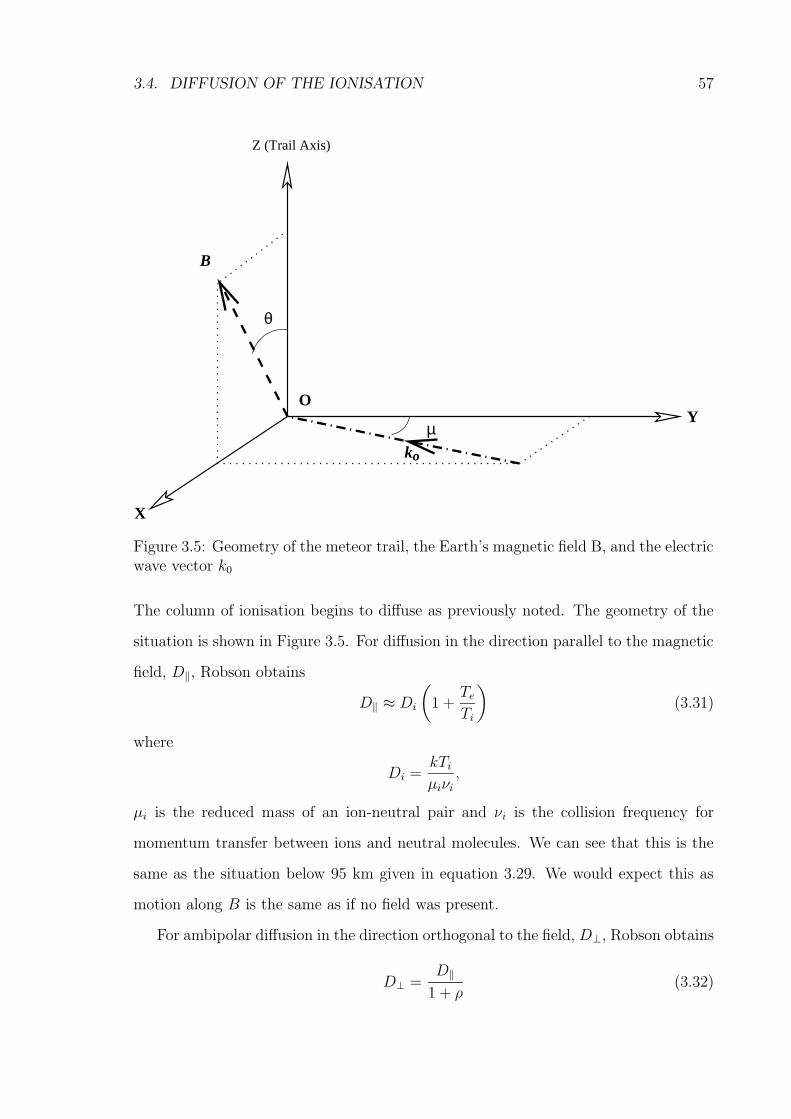
3.4. DIFFUSION OF THE IONISATION 57
θ
µ
B
O
k
X
Y
Z (Trail Axis)
o
Figure 3.5: Geometry of the meteor trail, the Earth’s magnetic field B, and the electricwave vector k0
The column of ionisation begins to diffuse as previously noted. The geometry of the
situation is shown in Figure 3.5. For diffusion in the direction parallel to the magnetic
field, D‖, Robson obtains
D‖ ≈ Di
(
1 +TeTi
)
(3.31)
where
Di =kTiµiνi
,
µi is the reduced mass of an ion-neutral pair and νi is the collision frequency for
momentum transfer between ions and neutral molecules. We can see that this is the
same as the situation below 95 km given in equation 3.29. We would expect this as
motion along B is the same as if no field was present.
For ambipolar diffusion in the direction orthogonal to the field, D⊥, Robson obtains
D⊥ =D‖
1 + ρ(3.32)

58 CHAPTER 3. RADIO METEOR THEORY
Figure 3.6: D‖ and D⊥ for a range of different heights. The value of the effectivediffusion coefficient will lie between these values depending on the orientation of thetrail (After (Elford & Elford 1999)). The line labelled S⊥ shows simulated values ofD⊥ at 2× 10¹⁴e m−1(After (Dyrud et al. 2001)).
where
ρ =e2B2
meνeµiνi,
me is the electron mass, and νe is the collision frequency for momentum transfer
between electrons and neutral molecules.
The ambipolar diffusion coefficients in the two directions can be combined together
into an effective diffusion coefficient, Deff , which is given by
Deff = D‖ sin2 µ sin2 θ +D⊥(1− sin2 µ sin2 θ) (3.33)
If we define φ as the angle that the magnetic field makes to the electric wave vector,

3.4. DIFFUSION OF THE IONISATION 59
then cosφ = sin θ sinµ, and:
Deff = D‖ cos2 φ+D⊥ sin2 φ (3.34)
The parallel and perpendicular diffusion coefficient can easily be calculated by using
empirically measured quantities such as free diffusion coefficients and mobilities of
electrons and ions in gases (Elford & Elford 1999, Elford & Elford 2001), and the
effective diffusion coefficient depends only on these and the angle of the radar beam
to the magnetic field.
Figure 3.6 shows the values of D‖ and D⊥ calculated in this way for a range
of different heights. The value of the effective diffusion coefficient will lie between
D‖ and D⊥. The values of D⊥ are calculated for three different values of the line
density, as for values greater than 1013 electrons per metre, the effects of Coulomb
interactions between electrons and ions must be considered. Also shown in Figure 3.6
is a line (labelled S⊥) of simulated values of D⊥ for 2×10¹⁴ electrons per metre (Dyrud
et al. 2001).
Oppenheim et al and Dyrud et al performed plasma simulations which showed
that density gradients at the edges of meteor trails drive gradient drift instabilities
which develop into waves with perturbed electric fields. These waves create an anoma-
lous cross field diffusion which can exceed D⊥ by an order of magnitude (Oppenheim
et al. 2000, Dyrud et al. 2001). This could significantly reduce the effect of the geo-
magnetic field in slowing diffusion and explain the lack of observations showing greatly
reduced diffusion coefficients at heights above 90 km1. The simulations have so far
been performed only for a trail line density of 2.0 × 10¹⁴e m−1. It is unclear whether
significant anomalous cross field diffusion will occur at lower levels of ionisation. Most
of the echoes detected with the Buckland Park VHF radar have electron line densities
which are less than 1013e m−1.
The increase in the lifetime of a radar echo due to the effects of the magnetic field,
1See Chapter 5 for observations which show greatly reduced diffusion coefficients!

60 CHAPTER 3. RADIO METEOR THEORY
1
10
100
1000
10000
0 10 20 30 40 50 60 70 80
Beam off-zenith angle (degrees)
Du
rati
on
en
han
cem
ent
(E)
90 km
95 km
100 km
105 km
110 km
120 km
Figure 3.7: Enhancement in the duration of meteor echoes due to the effect of theEarth’s magnetic field, calculated for electron line densities of 1013e m−1. At thelatitude of the Buckland Park VHF radar (35 S) the magnetic field lies at an angleof 68 to the horizontal.
E, can be calculated as:
E =Deff
D‖(3.35)
Applying this to the Buckland Park VHF radar, we obtain Figure 3.7, which shows
the increase in the lifetime of a radar echo observed with the South beam of the radar
directed to a number of different off-zenith angles, and for a number of different echo
heights. The enhancement is calculated for an electron line density of 1013e m−1. The
enhancement at a typical off-zenith angle of 30 is between 1.2 (at 90 km) and 2.6 (at
120km). In the first sidelobe, at an off-zenith angle of about 40, the enhancement
rises to 1.3 and 4.5 respectively.
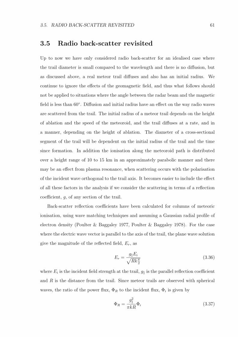
3.5. RADIO BACK-SCATTER REVISITED 61
3.5 Radio back-scatter revisited
Up to now we have only considered radio back-scatter for an idealised case where
the trail diameter is small compared to the wavelength and there is no diffusion, but
as discussed above, a real meteor trail diffuses and also has an initial radius. We
continue to ignore the effects of the geomagnetic field, and thus what follows should
not be applied to situations where the angle between the radar beam and the magnetic
field is less than 60. Diffusion and initial radius have an effect on the way radio waves
are scattered from the trail. The initial radius of a meteor trail depends on the height
of ablation and the speed of the meteoroid, and the trail diffuses at a rate, and in
a manner, depending on the height of ablation. The diameter of a cross-sectional
segment of the trail will be dependent on the initial radius of the trail and the time
since formation. In addition the ionisation along the meteoroid path is distributed
over a height range of 10 to 15 km in an approximately parabolic manner and there
may be an effect from plasma resonance, when scattering occurs with the polarisation
of the incident wave orthogonal to the trail axis. It becomes easier to include the effect
of all these factors in the analysis if we consider the scattering in terms of a reflection
coefficient, g, of any section of the trail.
Back-scatter reflection coefficients have been calculated for columns of meteoric
ionisation, using wave matching techniques and assuming a Gaussian radial profile of
electron density (Poulter & Baggaley 1977, Poulter & Baggaley 1978). For the case
where the electric wave vector is parallel to the axis of the trail, the plane wave solution
give the magnitude of the reflected field, Er, as
Er =g‖Ei√
Rk π2
(3.36)
where Ei is the incident field strength at the trail, g‖ is the parallel reflection coefficient
and R is the distance from the trail. Since meteor trails are observed with spherical
waves, the ratio of the power flux, ΦR to the incident flux, Φi is given by
ΦR =g2‖
πkRΦi (3.37)

62 CHAPTER 3. RADIO METEOR THEORY
"!
# $% &'()*+,
-.0/2143 5
6.0/2143 5
7.0/2143 5
Figure 3.8: Values of the attenuation factor for underdense echoes due to trail initialradius (αr) at various heights and meteoroid speeds calculated for a radar frequencyof 54.1 MHz (after (Jones 1995)).
and the power delivered to the receiver is
PR =g2‖PTGTGRλ
3
32π4R30
(3.38)
(Kaiser & Closs 1952, Eshelman 1955). For the case where the electric wave vector is
orthogonal to the trail, a similar expression can be obtained, by replacing calculated
values of g‖ with g⊥.
For trails above 90 km it is probably reasonable to assume initially a circular
cross-section for the ionisation, (although this doesn’t seem to have been examined
theoretically) and then determine g‖ as a combination of D‖ and D⊥
3.5.1 Attenuation factors for underdense echoes
There are several factors which determine the amplitude of the returned signal from
a meteor trail. For an underdense trail the reflection coefficient for a segment of the

3.5. RADIO BACK-SCATTER REVISITED 63
trail can be given by
g = qπre exp(−k2a2) (3.39)
where
a2 = 4Dt+ r20,
D and r0 are the diffusion coefficient and initial radius appropriate to the height of the
segment, and q is the line density in electrons per metre (Poulter & Baggaley 1978).
We assume that g = g‖ = g⊥ (which is true for q < 1012em−1 ). However Jones (1995)
has shown that the initial radius is not Gaussian, and has calculated an attenuation
factor due to the initial radius, αr, dependent on the atmospheric number density, na,
the meteoroid velocity, v, and the radio wavelength, λ, giving a new expression for the
reflection coefficient,
g = qπreαr exp(−4k2Dt) (3.40)
Figure 3.8 shows the value of αr calculated for a frequency of 54.1 MHz, at a number
of different heights and for meteoroid speeds of 20, 40 and 60 km s−1. The most
striking features of the plot are that αr = 0.5 at 90-95 km, and the suggestion that no
underdense meteor trails are detectable above 105 km. This factor has the greatest
effect on the observed height distribution, but the significance of the effect is dependent
on a better understanding of the shape of the trail cross-section and the magnitude
of the effective initial radius. Jones predicts that trails are formed with a well defined
core surrounded by diffuse ionisation. The observed height distribution discussed in
Section 5.3 reveals the presence of a significant number of underdense echoes above
105 km, suggesting that Jones’ core is “more concentrated” than he predicts.
Since the meteoroid is travelling with a finite speed, the trail is diffusing while the
central Fresnel zone is being formed, and there will be a reduction in the value of the
reflection coefficient with the increase in distance from the point of formation of the
trail (Kaiser 1953). The attenuation, αv, due to this effect can be approximated by
αv =1− exp(−∆)
∆, (3.41)

64 CHAPTER 3. RADIO METEOR THEORY
where
∆ =2k2D
√2Rλ
v,
R is the range in metres and v in the speed of the meteoroid (Peregudov 1958).
Once the trail has been formed, the returned echo power from an underdense trail
will decay due to diffusion. This raises the possibility that a trail formed just after
the passage of a transmitted pulse may not be detected by the next pulse, if the decay
time is comparable to the interpulse period. The average attenuation factor for this
effect can be given as:
αP =
(
1− 1
expw2
)
1
w1
(3.42)
where
w1 =4(s− 1)k2D
p,
w2 =4k2D
p,
s is the mass index of the meteoroids, k = 2π/λ, D is the diffusion coefficient and p is
the pulse repetition frequency in Hz.
3.5.2 Faraday rotation
Another attenuation factor is the effect of the ionosphere on the passage a radio waves.
The Ionosphere below a meteor trail acts as a doubly refracting medium, and during the
day, when the ionisation is highest, the ordinary and extraordinary waves may become
manifest as two pulses with different amounts of retardation and absorption. For
frequencies above 15 MHz, this produces Faraday rotation of the plane of polarisation.
The amount of rotation occurring on linearly polarised signals reflected from meteor
trails depends on the integrated ionisation over the path of the signal, the orientation
of the path to the magnetic field and radio frequency (Budden 1985). The effect can
be estimated by using a quasi-longitudinal approximation to the ionospheric refractive
index. This gives the following expression for Ω, the Faraday rotation in radians

3.5. RADIO BACK-SCATTER REVISITED 65
between the ground and the trail,
Ω = 2.36× 10⁴ 1
f 2
∫
path
B cosχ N(s)ds (3.43)
where f is the wave frequency, B is the local geomagnetic field, χ is the angle between
the wave propagation direction and the direction of B, N is the electron density,
and ds is a path element. In the case of back-scatter the total Faraday rotation is
2Ω, and if the transmitting and receiving antennas have common linear polarisations,
then the amplitude of the returned signal is reduced by a factor αF = cos(2Ω). In
general, calculations of Faraday rotation need to be based on the full Appleton-Hartee
expressions for the refractive index, including losses due to collisions. The amount of
Faraday rotation can exceed 90 during the daytime, and this will manifest itself by
reducing the amplitude of the returned signal to zero for certain ranges, depending
on the elevation and azimuth of the reflection point, the time of day, the location of
the radar (ie. the angle of the geomagnetic field) and the solar activity (Elford &
Taylor 1997).
3.5.3 Overdense meteor trails
The Buckland Park VHF radar is able to observe meteor trails with a limiting electron
line density of about 1010electron/m and the transition from underdense to overdense
trail begins at about 1013electrons/m. This implies that most of the echoes which
will be observed by the radar will be underdense. As such only a brief discussion will
be given on overdense trails here; for a fuller discussion, see McKinley (1961) and
Ceplecha et al. (1998).
For overdense trails the reflection can be considered to be taking place at the
surface of a cylinder in which the dielectric constant is negative. Ceplecha et al give
a value for the maximum reflection coefficient for an overdense trail where (g‖)ov ∼=
7.5× 10⁻⁵q0.275. This gives a line density dependence for the echo power of q0.55 over
a range of line densities from 1014 to 1016m−1, much smaller than the underdense case
where PR ∼ q2. While the trail is overdense, the returned echo is not subject to the

66 CHAPTER 3. RADIO METEOR THEORY
effects of initial radius and diffusion, although diffusion is what causes the “reflecting
surface” to expand.
The full expression for the received echo power from an overdense trail is
PR = (g‖)2ov
PTGTGRλ3
32π4R30
= 1.8× 10⁻¹²PTGTGR
(
λ
R0
)3
q0.55 (3.44)
For the case of overdense trails occurring at heights above 95 km, the effect of the
geomagnetic field must be taken into account. This has the effect of changing the
shape of the reflecting surfaces to have an elliptical cross-section with the major axis
lying in the plane containing the axis of the trail and the direction of the magnetic
field.
A radio echo from an overdense trail will endure for as long as the electron volume
density is above the critical density for the wavelength being used. The depletion
of the ionisation is controlled by ambipolar diffusion above 93 km and by chemical
destruction below 93km (Baggaley 1980). The main chemical process is the reaction
of meteoric ions with ozone to form oxide ions which rapidly recombine dissociatively
with the free electrons. Jones et al. (1990) have shown that the duration distribution
of overdense echoes at a given height has a “characteristic time”, corresponding to the
changeover from “diffusion limited” to “chemistry limited” durations. Observations of
the duration of overdense echoes can be used to determine the concentration of ozone
at various heights in the meteor region of the atmosphere.
3.6 The Radar response function
It is necessary to be able to interpret radar meteor echo rates in terms of the flux
of meteoroids entering the atmosphere. Each echo provides a number of parameters,
namely the range and time of occurrence, together with one or more of the amplitude,
phase, duration and direction of arrival of the echo. In order to be able to interpret this
data the response of the radar to the meteor flux must be determined. A meteor trail
which is formed inside the radiation pattern of a radar will be detected if it satisfies

3.6. THE RADAR RESPONSE FUNCTION 67
the conditions of specular reflection, (ignoring “down the beam” echoes) and if the
returned power and duration are larger than the detection levels.
The response of the radar as a function of the radiant position of meteors is called
the response function. This function can be calculated as the theoretical echo rate for
a point source radiant of unit strength determined for all positions of the radiant in
the sky. The factors which determine the response function are the antenna pattern,
the ionisation profiles of meteors, the polarisation of radio waves with respect to the
meteor trail, the elevation of the meteor radiant, the minimum detectable electron
line density of the radar, the detection criteria for the system, attenuation factors (as
discussed in Sections 3.5.1and 3.5.2) and the flux of meteors as a function of mass or
zenithal line density.
As the majority of meteors detected by the Buckland Park VHF radar will be un-
derdense, we can assume that the echo amplitude is proportional to the electron line
density at the reflection point, modified by the attenuation factors previously men-
tioned. In Section 3.1.2, it was shown that meteoroids of a given speed tend to produce
trails at the same height regardless of mass, for the size range of meteoroids detected
by the Buckland Park VHF radar (corresponding to the flat sections in Figure 3.1).
The trails extend over a height range of 10 to 15 km, and the ionisation distribution
is well approximated by a parabolic function of the density of the atmosphere at the
height of maximum ionisation.
3.6.1 The radar response function for the Buckland Park VHF
radar
The derivation of the response function for back-scatter radar has been previously
carried out (Elford 1964, Thomas et al. 1988, Elford et al. 1994). The basis for this
model relies on modelled meteors with idealised ionisation profiles of constant line
density over a given height range (Kaiser 1960). Cervera (1996) developed the response
function for the Buckland Park VHF radar in great detail, so only a general overview

68 CHAPTER 3. RADIO METEOR THEORY
N
B
L
A
C
D
θ
φ
χo
r
r
P
Radiant Direction
Θ
hh
1
2
dS
RΦ
Figure 3.9: Geometry for the condition for specular back-scatter. The Radiant is atan azimuth angle of φr and elevation of θr. The plane ABCD is orthogonal to theradiant direction.
will be given here. Cervera had a hardware limit on the maximum range detectable by
the radar, but this problem has been resolved with the radar data acquisition system
upgrade, and this change has been factored into the new radar response function
The response function calculation makes use of the conditions for specular reflec-
tion, the geometry of which is shown in Figure 3.9. For a specular reflection from a
trail produced by a meteoroid coming from the direction of the radiant, which has
an azimuth angle of φr and elevation of θr, all possible echo points lie in the plane
defined by ABCD. All meteors with the same speed are assumed to ablate over the
same height range, beginning at h2 and ending at h1. This constrains the echoes to
a thin strip of the echo plane. Point P is an echo point and is within an area dS in
the echo plane. P is at a range R, elevation angle Θ, height h and echo plane azimuth

3.6. THE RADAR RESPONSE FUNCTION 69
angle Φ as measured in the plane.
We assume that the cumulative flux of meteoroids above a certain mass from a
unit area of the sky, per steradian per second, is a power law of the form:
N(m) = Kmc∞ (3.45)
where m∞ is the limiting initial mass of the meteoroid, which is obtained from the
minimum detectable electron line density and ablation theory. Various values for
parameter c have been estimated (McKinley 1951a, Weiss 1961, Kaiser 1953, Kaiser
1961, Elford 1964, Thomas et al. 1988), with the values changing dependent on the
mass of the particles. For underdense radar meteors the results tend toward a value
of c ≈ −1.0. K is a multiplicative factor for which the actual value is not needed as
we are only interested in the relative response of the radar.
The echo rate from radiants lying within a solid angle dΩ about a radiant direction
with elevation θr and azimuth φr is:
n(θr, φr) dΩ =
∫
echoplane
N(m) dS dΩ (3.46)
The function n(θr, φr) is the response of the radar to a meteor radiant of unit density
in the direction (θr, φr), ie the responsefunction. Using the polar coordinates, R and
Φ, for the reflection point, P, we have:
dS = R dΦ dR (3.47)
Taking into account the curvature of the Earth, we use Figure 3.10 to give us the
range:
R = RE
(√
sin2 θ +2h
RE
+h2
R2E
− sin θ
)
(3.48)
Substituting 3.47 and 3.48 into 3.46 gives:
n(θr, φr) = REK
∫ h2
h1
∫ π2
−π2
mc∞f(Φ)
(
1 +h
RE
)
dΦ dh (3.49)
where
f(Φ) = 1− cos θr cosΦ
(
cos2 θr cos2 Φ +2h
RE
+h2
R2E
)−1/2
(3.50)

70 CHAPTER 3. RADIO METEOR THEORY
θ
P
L
h
O
RE
R
Figure 3.10: Geometry for a reflection point, P, with respect to the Earth’s curvedsurface
The limiting initial mass of the meteoroid, m∞ is obtained from the limiting de-
tectable electron line density and classical ablation theory, both which introduce a
dependence on velocity. The limiting electron line density for underdense meteors is
given by:
qmin = 4.5× 10¹⁵
(
R
λ
)3/2√
PRPTGT (θ, φ)GR(θ, φ)αrαvαPαF
(3.51)
where αr, αv, αP and αF are the attenuation factors described in Sections 3.5.1 and
3.5.2.
McKinley discusses ablation ignoring the effects of radiation and vapour pressure
and assuming no deceleration of the meteoroid (McKinley 1961). From (7.10) and
(7.15) we can write :
q(h) = k2ρa(m13∞ −
k1p
cosχ) (3.52)

3.6. THE RADAR RESPONSE FUNCTION 71
where ρa and pa are the density and pressure of the atmosphere as a function of height,
the geometric height is h, χ is the angle the path of the meteoroid makes with the
zenith, and k1 and k2 are constants for a particular meteoroid composition, and are
given by:
k1 =ΛAv2
6Lgρ2/3m
,
k2 =3βgk1
µ.
where g is the acceleration due to gravity and the other variables are as previously
defined.
This leads to an expression for the limiting initial mass of the meteoroid ignoring
the effects of radiation and vapour pressure on ablation as follows:
m∞ =
(√
q
k2ρa+k1pacosχ
)3
(3.53)
If we rewrite Equation 3.52 in terms of the maximum values of the line density,
qmax, and the atmospheric pressure, pmax, at the height where the line density is a
maximum:
qmax =4
9
β cosχ
µHmax
m∞ (3.54)
pmax =1
3
cosχ
k1
m13∞ (3.55)
where Hmax is the scale height at pmax. Thus 3.52 becomes:
q
qmax=
9
4
p
pmax
(
1− p
3pmax
)2
(3.56)
If we use Q = q/qmax and P = p/pmax then we can write:
Q =9
4P (1− P/3)2 (3.57)
This is the “Classical” ionisation profile, with zero ionisation at P = 0 and 3, and a
maximum at P = 1. It is clearly unrealistic, as it indicates that ionisation starts when
the atmospheric pressure is zero.
Modelling of the ablation of a meteoroid, including radiation losses, shows that
the commencement of ionisation occurs for values of P ranging from 0.05 for large

72 CHAPTER 3. RADIO METEOR THEORY
meteoroids to 0.3 for small meteoroids, and ceases (for small meteoroids) at values as
low as 1.9 (Love & Brownlee 1991). By comparing the ionisation profiles calculated for
a range of particle masses, Elford (private communication) has produced the following
expression in the form of Equation 3.57:
Q = K(P − P0)
(
1− P
3− 3P0
)2
(3.58)
Where K = 9(1− P0)(2− 3P0)−2, and expressions for P0 are as follows:
P0 =
−3.69× 10⁻² lnm∞ − 0.55 for m∞ < 2× 10⁻⁸kg
−1.52× 10⁻² lnm∞ − 0.175 for m∞ ≥ 2× 10⁻⁸kg
The modelling also showed that the classical expressions for qmax and pmax given
above must be modified. In particular, in the expression for pmax, the exponents of
m∞ and cosχ become 0.22 and 0.53 respectively. The dependence of qmax on m∞ and
cosχ is unchanged, but there is an additional dependence on v in the form v0.43, giving
qmax a total dependence on v of v3.42v0.43 = v3.85 (the v3.42 dependence is contained
in the factors β and Hmax). For a given value of m∞, the corresponding qmax can be
calculated, and the limiting initial mass can be determined.
A simplified response function has been given by Elford et al. (1994) for narrow
beam systems. f(Φ) is a slowly varying function of Φ, and for a narrow beam system
can be approximated by a mean value when integrating over the echo plane. By
including all the constants into K, and for the case where the same antenna is used
for transmission and reception ( ie GT = GR = G), they obtain:
n(θr, φr) = K∆h sin θrf(Φ)
∫
GdΦ (3.59)
where f(Φ) is the mean value of that function, and ∆h implies a range of ablation
heights is taken into account (the mean height is included in the constant K).
3.6.2 Calculation of the Response Function
The response function for typical configurations of the Buckland Park VHF radar and
different initial speeds has been calculated by Cervera (1996). Investigation of different
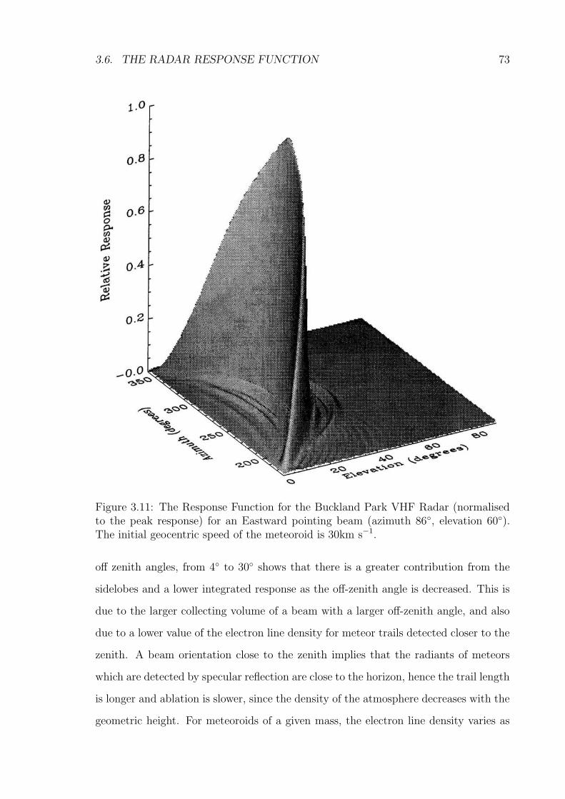
3.6. THE RADAR RESPONSE FUNCTION 73
Figure 3.11: The Response Function for the Buckland Park VHF Radar (normalisedto the peak response) for an Eastward pointing beam (azimuth 86, elevation 60).The initial geocentric speed of the meteoroid is 30km s−1.
off zenith angles, from 4 to 30 shows that there is a greater contribution from the
sidelobes and a lower integrated response as the off-zenith angle is decreased. This is
due to the larger collecting volume of a beam with a larger off-zenith angle, and also
due to a lower value of the electron line density for meteor trails detected closer to the
zenith. A beam orientation close to the zenith implies that the radiants of meteors
which are detected by specular reflection are close to the horizon, hence the trail length
is longer and ablation is slower, since the density of the atmosphere decreases with the
geometric height. For meteoroids of a given mass, the electron line density varies as

74 CHAPTER 3. RADIO METEOR THEORY
Figure 3.12: The Response Function for the Buckland Park VHF Radar for an East-ward pointing beam (azimuth 86, elevation 60). The initial geocentric speed of themeteoroid is 30km s−1 In panel (a) the contours show the relative response as a frac-tion of the peak response as a function of elevation and azimuth. Panel (b) shows therelative response at an azimuth of 266.
cosχ where χ is the zenith angle of the radiant. This means that the sidelobes with
larger off-zenith angles than the main beam have a greater response than those with
smaller off-zenith angles, in the ratio about four to one. The total response of the
sidelobes is less than 10 % of the response of the main beam.
Figure 3.11 shows the response function as a surface. The main lobe is due to
the main beam of the antenna pattern that is directed to 86 in azimuth and 60 in
elevation. The main feature of the response function is a curved wedge extending from
azimuth 176 to 356, with a maximum at azimuth 266. The conditions for specular
back-scatter require that the meteor trail be orthogonal to the beam direction, and
there is a range of radiants which satisfy this. Out of these, the radiants which are
closer to the horizon, produce a lower response, as previously explained, thus the fall
off in response toward the ends of the wedge. Figure 3.12 shows the response function

3.7. SUMMARY 75
as (a )a contour plot and (b) against elevation. In panel (a) the contours shows the
relative response as a fraction of the peak response. Panel (b) shows the relative
response at an azimuth of 266; note the asymmetry in the sidelobes.
Investigations of the effect of the initial speed of the meteoroid showed two effects,
the first was an increase in the response in the sidelobes with speed and the second
was a rise in the peak response up to a speed of 40km s−1 followed by a fall off. As the
initial speed of a meteoroid increases, the ionisation efficiency increases as vn, where
n is between 3.5 and 4.0 (Bronshten 1983, McKinley 1961, Verniani 1973). The height
of ablation also increases. These two factors compete against each other, in that more
ionisation increases the detectability of the meteor, but a greater height of ablation
brings a greater attenuation of the returned signal from the meteor trail2. At speeds
above 40kms−1 the attenuation factors dominate, and because the sidelobe sensitivity
is much lower than the main beam, mainly overdense echoes should be detected, on
which the attenuation factors have little effect.
3.7 Summary
In this chapter, theory relating to the reflection of radio waves from meteor trails
has been expounded. First was ablation theory, which describes how meteoroids heat
and ablate as they travel through the atmosphere, including a survey of previous
models. The differential equations of motion model how a meteoroid gains and loses
heat and then loses material as it decelerates. An analytical solution to the equations
is described, including corrections for deceleration. Added to the model were the
effects of fragmentation during flight based on observations which showed behaviour
inconsistent with the earlier model.
The formation of the ionised trail and the effects of the initial radius of the meteor
trail were discussed, the initial radius being the RMS radius of the ionisation column
formed when the ablated atoms are decelerated rapidly by collision with atmospheric
2See Section 5.3 for further discussion on the true effect of the initial radius attenuation factor

76 CHAPTER 3. RADIO METEOR THEORY
molecules. The effects of the radial distribution of the ionisation and the use of an
effective initial radius were introduced.
Underdense trails were defined as trails in which the electron line density is low
enough to ensure that secondary scatter of radio waves is insignificant. Overdense
trails were defined such that this secondary scatter is significant, and they can be
modelled as a metallic cylinder. The geometry of radio wave scatter from meteor
trails was discussed in relation to the condition of specular reflection, through which
most meteor echoes are obtained, and the less frequent case of “down the beam”
echoes, where the meteor is observed as a hard target passing through the beam. A
basic model of radar back-scatter from underdense meteor trails using Fresnel theory
is described, with some discussion of the effects of fragmentation.
When the ionised trail has formed, it begins to dissipate, mostly due to the effects
of ambipolar diffusion. New work on diffusion including the effects of the Earth’s
magnetic field shows that at heights above 95 km this can have a significant effect
on the lifetimes of meteor trails, but the extent of this effect is uncertain due to the
formation of gradient-drift instabilities at the edges of meteor trails.
Attenuation factors caused by the initial radius, diffusion, the finite speed of the
meteoroid, the PRF of the radar and the effects of Faraday rotation are defined. Also
discussed was radar back-scatter from overdense meteor trails.
Lastly the radar response function was developed, and calculated for the Buckland
Park VHF radar, including the effects of different zenith angles and different initial
meteoroid speeds. It was shown that best results are obtained from off-zenith tilts of
more than 20 and that at higher speeds the increase in ablation height and the effects
of attenuation factors causes a bias against underdense echoes. Further uses of the
response function will be introduced in subsequent chapters.

Chapter 4
Data processing
Once the data is stored on the hard disk of the PC dedicated to meteor data acquisition,
it can then be transformed into various characteristics of the meteor echo. The data
files are stored as a sequence of “inphase” and “quadrature” values, with a header
for each echo describing the radar operating conditions at the time of the record.
A program was written in IDL, an array based programming language developed by
Research Systems, Inc., which would take these values, turn them into amplitude and
phase values, and then plot them on the screen. This was done by the vector addition
of the inphase and quadrature values, the amplitude being the length of the resultant
and the phase being the angle as follows.
Amplitude =√
Inphase2 +Quadrature2
Phase = arctan
(
Inphase
Quadrature
)
There were a number of other sections written into the code to perform various “house-
keeping” functions. A number of these involved procedures for plotting, expanding and
printing the data. These sections will not be expanded upon, as the techniques used
are very simple even if producing code to perform them is not.
Matters discussed in this chapter involve phase unwrapping, the removal of periodic
noise and coherent smoothing. Other matters involving the analysis of the meteor
77

78 CHAPTER 4. DATA PROCESSING
echoes to obtain speeds, ambipolar diffusion coefficients and radial wind drifts will be
discussed in chapters 5 and 6. Also in this chapter are discussions on the effect of
receiver saturation and the effect random noise on the signals. The IDL code which
performs all these functions is available on the CDROM in the back cover of this
volume.
4.1 Phase unwrapping
The program contained a section to “unwrap” the phase values. This was carried
out because all values of phase for each pulse of data lie between π and −π radians,
although the phase values are actually continuously varying over many cycles. A cycle
of 2π radians represents a total distance change of the returned signal of one wave-
length, 5.454 m. For backscatter, the actual range change is one half wavelength. The
unwrapping algorithm simply checks if the difference in phases between two adjacent
points is greater than π and if so, adds or subtracts 2π from the second point. Figure
4.1 shows the result of this in the panel “unwrapped phase”. While it is evident that
this simple method is surprisingly effective, it has two limitations. The first is that
point to point phase changes of more than 2π are not corrected. Secondly, random
noise which decreases the value of the phase “jump” between two points to less than
2π causes that “jump” to be neglected, producing a “step” in the phase record.
The algorithm was improved by allowing an integral number of 2π cycles to be
added or subtracted, subject to the condition that the change produces greater con-
sistency in the slope of the phase record. This involves working backwards through
the phase series and considering the effect on each point of adding a phase change of
±n2π, where n is an integer. If one of these changes brings the slope at this point
closer to the average slope for the several previous points, the change is retained. The
effect of this procedure is shown in Figure 4.1, producing the result shown in the panel
labelled “new unwrapping”. The previously described unwrapping is also plotted in
the panel for comparison. The phase change is unwrapped through many more cycles

4.1. PHASE UNWRAPPING 79
Figure 4.1: A transverse meteor echo showing the effect of phase unwrapping. Shownfrom top to bottom panels are: amplitude, phase, simple unwrapped phase and thenew phase unwrapping. See text for further details
than in the previous unwrapping, and the parabolic shape of the unwrapped phase is
precisely as we would expect from Fresnel theory of radar back-scatter (see Section
3.3.3 and Figure 3.4
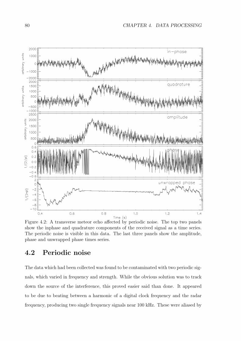
80 CHAPTER 4. DATA PROCESSING
Figure 4.2: A transverse meteor echo affected by periodic noise. The top two panelsshow the inphase and quadrature components of the received signal as a time series.The periodic noise is visible in this data. The last three panels show the amplitude,phase and unwrapped phase times series.
4.2 Periodic noise
The data which had been collected was found to be contaminated with two periodic sig-
nals, which varied in frequency and strength. While the obvious solution was to track
down the source of the interference, this proved easier said than done. It appeared
to be due to beating between a harmonic of a digital clock frequency and the radar
frequency, producing two single frequency signals near 100 kHz. These were aliased by

4.2. PERIODIC NOISE 81
sampling at the pulse repetition frequency to a large amplitude single-frequency signal
and a smaller one. These signals changed slowly with time in both strength and in
frequency, sometimes coming close enough to form meteor-like shapes by beating and
fooling the detection algorithm. While a correction of the design fault that generated
the periodic noise in the system would have been the ideal solution to this problem,
this was outside the author’s control as the equipment was timed shared with other
programs for which the periodic noise was not a significant problem. Thus the reduc-
tion of the periodic noise was carried out as part of the meteor signal processing, with
an excellent outcome. Figure 4.2 shows a transverse meteor echo in which the periodic
noise is obvious in the inphase and quadrature time series. The periodic noise is also
plainly visible in the amplitude and phase data during the decay of the meteor echo
from 0.7 to 1.1 seconds.
A procedure to reduce the effect of the periodic noise was developed and automat-
ically applied to the data. Its efficacy can be seen by comparing the “cleaned” set of
data in Figure 4.3 with the original data in Figure 4.2. The periodicity in the time
series is no longer visible. The most important effect is on the phase series, where the
noise reduction removes most of the errors in the phase unwrapping, giving a pre-t0
curve where there wasn’t one before.
The procedure to remove the noise is as follows. Firstly the inphase and quadrature
data are transformed into power spectra by using a fast Fourier transform (FFT). Then
the three sharpest peaks in each power spectrum are located. The “sharpness” of the
peaks is defined by user input, but should be sharp enough to ignore the meteor signal.
Peaks which are found at the same frequency in both spectra are taken to be periodic
noise and are removed from the power spectra by:
• Replacing the amplitudes of the frequency components with some values copied
from a nearby part of the frequency spectrum.
• Replacing the phase values of these frequency components with random values
• Transforming the modified complex spectra back to the time domain, to give

82 CHAPTER 4. DATA PROCESSING
Figure 4.3: This is the transverse meteor echo shown in Figure 4.2, with periodic noisereduction applied. The top two panels show the inphase and quadrature componentsof the received signal as a times series. The last three panels show the amplitude,phase and unwrapped phase times series.
corrected inphase and quadrature time series.
4.3 Coherent smoothing
Since there is random noise in the signals, very weak signals can be hard to discern
from the background. The usual way to increase the signal-to-noise ratio is to perform

4.3. COHERENT SMOOTHING 83
Figure 4.4: Power spectrum of a transverse meteor echo before and after periodic noisereduction. The peaks at frequencies of 50 and 305 Hz are plainly visible in the toppanel.
smoothing of the data, and this feature was introduced into the meteor analysis pro-
gram. One method used was to perform a sliding boxcar coherent average of the data
with the size user definable. This is performed, for a point number n, point value A,
using the following expression,
A′(n) =A(n) + A(n+ 1) + A(n− 1) + . . . A(n+ x/2) + A(n− x/2)
x(4.1)
where x is the size of the boxcar (in terms of the number of pulses defined by the
user) and A′ is the new value of the point. This was performed on the inphase and
quadrature data before it was converted to amplitude and phase, as this gives a better
signal-to-noise ratio than performing the smoothing directly on the amplitude and
phase data (Cervera 1996). The effect of coherent smoothing on the meteor echo
from Figure 4.3 is shown in Figure 4.5, where the signal-to-noise ratios of both the
amplitude and phase signals are greatly improved after the application of a 10 point
sliding boxcar coherent average. This smoothing was not applied routinely, as it

84 CHAPTER 4. DATA PROCESSING
Figure 4.5: The meteor echo from Figure 4.3 showing the effect of a 10 point slid-ing boxcar coherent average applied to the data. Note the vast improvement to theamplitude and phase signal-to-noise ratios
tended to reduce the effectiveness of the unwrapping code, by “rounding over” the
2π discontinuities, producing steps or jumps in the unwrapped phase record. When
smoothing was applied, it was found that a boxcar size of three points was the most
effective for increasing signal to noise without disturbing the phase unwrapping, and
in fact it sometimes improved the phase unwrapping.
Another smoothing method used, was to take the median value of x points about n
and assign that value to the point at n. This had a very similar effect to the previously
described method, but tended to be useful where there was a point in the data with a
much greater value than the surrounding points. These points have a great effect on
mean value, but the median is unaffected by this situation.

4.4. THE EFFECTS OF RECEIVER SATURATION 85
4.4 The effects of receiver saturation
As previously stated, the receiver produces a signal in the form of inphase and quadra-
ture components. It is necessary to investigate the effect of receiver saturation on the
recorded signals. The gain of the receiver is set to a high level in order to detect the
smallest possible returns, but this means that echoes which have very high returned
power will cause the receiver to saturate. The electron line density of a meteor is pro-
portional to its mass and increases as a power of the velocity. In turn the probability of
a certain mass varies approximately as the inverse of the mass, and the velocity has a
similar distribution (Taylor 1995). This means that there is a much higher probability
of small amplitude echoes than large, so the rate of saturated echoes should be small.
A survey of 13679 meteor echoes recorded in 1998, over 77 days of observations (1641
hours) revealed only 419 saturated meteor echoes, a rate of one every 3.9 hours of
observation (compared to the total average rate of one every 7.2 minutes). Saturated
meteor echoes were about 3% of the total number of echoes. Despite this small per-
centage, it is important to determine the effect of saturation in order to see if it will
affect speed measurements.
In Figure 4.6 we see the effect of saturation on a signal. The vector ‘A’ describes a
signal with constant unsaturated amplitude A and varying phase. Each panel shows
the signal at successively increasing times, with the dashed box enclosing the region
where the inphase and quadrature components are not saturated. In panel (a) the
signal has a phase such that the quadrature component is less than the upper boundary
of the dashed box, and as such is not saturated. However the inphase component
exceeds the right boundary of the box, and is therefore saturated. The actual signal
observed is found by truncating the inphase component to the limiting level, and this
saturated signal is labelled A’. Note that A’<A, and the phase of the saturated signal
is different (in this case advanced) to the true phase of the signal. In panel (b) we
see that a short time later, although the quadrature component has not started to
saturate, the saturated amplitude and the error in the phase have both increased. In
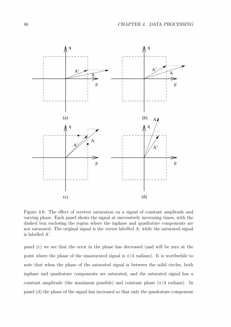
86 CHAPTER 4. DATA PROCESSING
q
p
q
p
q
p
q
p
A’A
A’A
A’A
A’
A
(c) (d)
(b)(a)
Figure 4.6: The effect of receiver saturation on a signal of constant amplitude andvarying phase. Each panel shows the signal at successively increasing times, with thedashed box enclosing the region where the inphase and quadrature components arenot saturated. The original signal is the vector labelled A, while the saturated signalis labelled A’.
panel (c) we see that the error in the phase has decreased (and will be zero at the
point where the phase of the unsaturated signal is π/4 radians). It is worthwhile to
note that when the phase of the saturated signal is between the solid circles, both
inphase and quadrature components are saturated, and the saturated signal has a
constant amplitude (the maximum possible) and constant phase (π/4 radians). In
panel (d) the phase of the signal has increased so that only the quadrature component
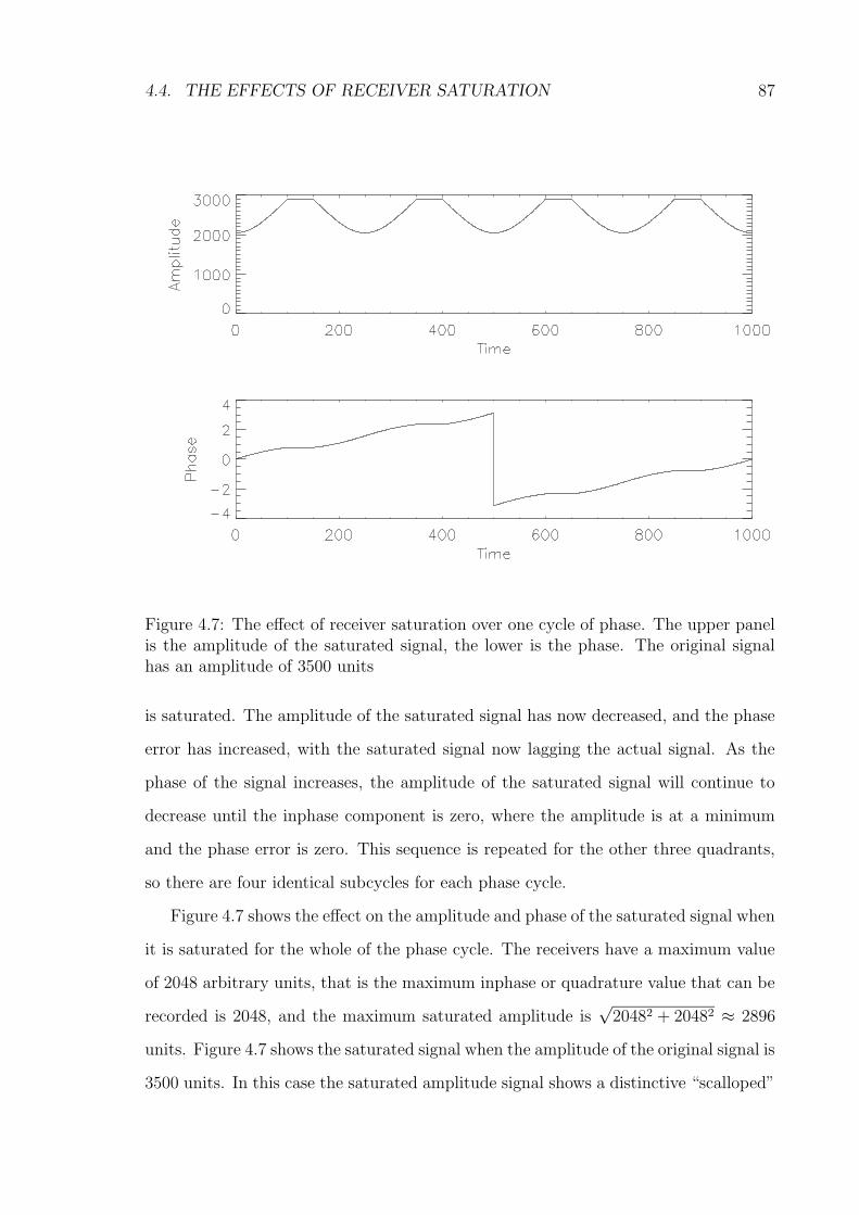
4.4. THE EFFECTS OF RECEIVER SATURATION 87
Figure 4.7: The effect of receiver saturation over one cycle of phase. The upper panelis the amplitude of the saturated signal, the lower is the phase. The original signalhas an amplitude of 3500 units
is saturated. The amplitude of the saturated signal has now decreased, and the phase
error has increased, with the saturated signal now lagging the actual signal. As the
phase of the signal increases, the amplitude of the saturated signal will continue to
decrease until the inphase component is zero, where the amplitude is at a minimum
and the phase error is zero. This sequence is repeated for the other three quadrants,
so there are four identical subcycles for each phase cycle.
Figure 4.7 shows the effect on the amplitude and phase of the saturated signal when
it is saturated for the whole of the phase cycle. The receivers have a maximum value
of 2048 arbitrary units, that is the maximum inphase or quadrature value that can be
recorded is 2048, and the maximum saturated amplitude is√20482 + 20482 ≈ 2896
units. Figure 4.7 shows the saturated signal when the amplitude of the original signal is
3500 units. In this case the saturated amplitude signal shows a distinctive “scalloped”
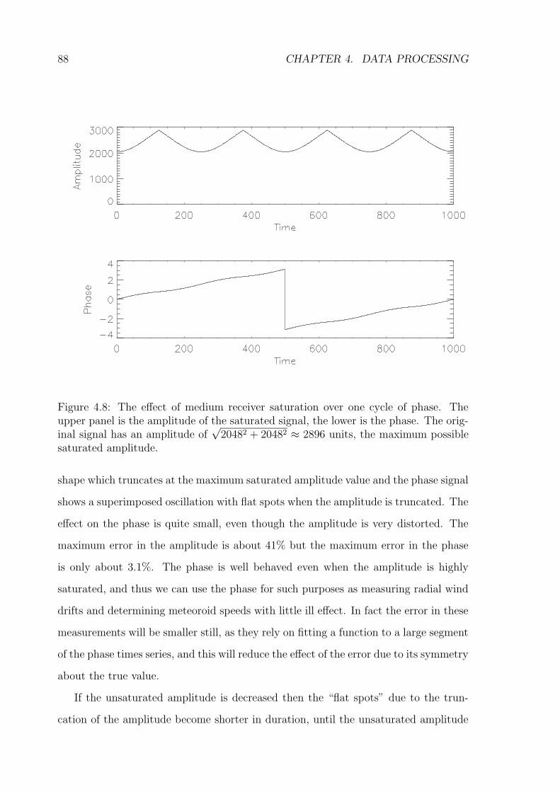
88 CHAPTER 4. DATA PROCESSING
Figure 4.8: The effect of medium receiver saturation over one cycle of phase. Theupper panel is the amplitude of the saturated signal, the lower is the phase. The orig-inal signal has an amplitude of
√20482 + 20482 ≈ 2896 units, the maximum possible
saturated amplitude.
shape which truncates at the maximum saturated amplitude value and the phase signal
shows a superimposed oscillation with flat spots when the amplitude is truncated. The
effect on the phase is quite small, even though the amplitude is very distorted. The
maximum error in the amplitude is about 41% but the maximum error in the phase
is only about 3.1%. The phase is well behaved even when the amplitude is highly
saturated, and thus we can use the phase for such purposes as measuring radial wind
drifts and determining meteoroid speeds with little ill effect. In fact the error in these
measurements will be smaller still, as they rely on fitting a function to a large segment
of the phase times series, and this will reduce the effect of the error due to its symmetry
about the true value.
If the unsaturated amplitude is decreased then the “flat spots” due to the trun-
cation of the amplitude become shorter in duration, until the unsaturated amplitude

4.4. THE EFFECTS OF RECEIVER SATURATION 89
Figure 4.9: The effect of minor receiver saturation over one cycle of phase. The upperpanel is the amplitude of the saturated signal, the lower is the phase. The originalsignal has an amplitude of less than the maximum value of the saturated amplitudeat 2300 units
reaches the critical value, the maximum saturated amplitude, about 2896 units. Fig-
ure 4.8 shows one cycle of phase when the unsaturated amplitude has this value. The
“flat spots” have disappeared, and the maximum error in the phase has reduced still
further to about 1.7%. The unsaturated phase and amplitude have the same values as
the saturated phase and amplitude at discrete points, namely when the value of the
phase is an integer multiple of π/4.
Further reduction in the unsaturated amplitude leads to the example shown in
Figure 4.9, where the unsaturated amplitude has a value of 2300 units. Here the
saturated amplitude agrees with the unsaturated amplitude for much of the time,
“dropping out” when one of the components saturates. The error in the phase is now
so small (about 0.3%) that the deviation from the true value is difficult to see in the
Figure. Although it has a similar appearance to Figure 4.7, the “flats spots” in Figure
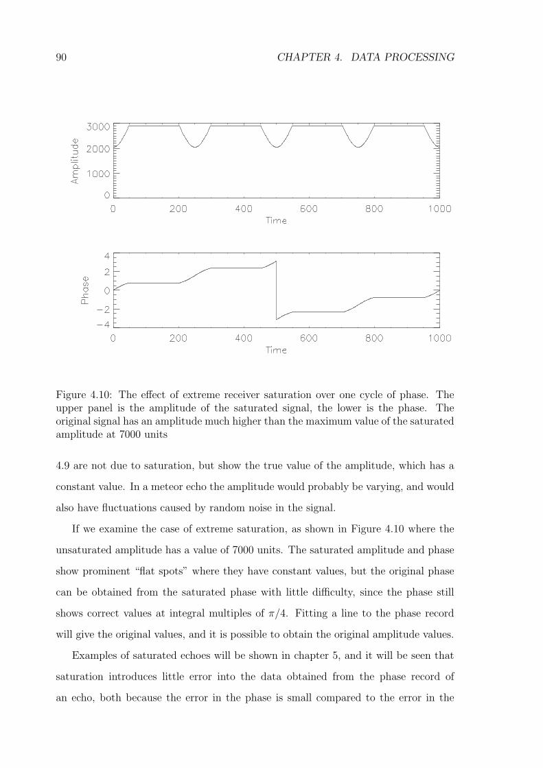
90 CHAPTER 4. DATA PROCESSING
Figure 4.10: The effect of extreme receiver saturation over one cycle of phase. Theupper panel is the amplitude of the saturated signal, the lower is the phase. Theoriginal signal has an amplitude much higher than the maximum value of the saturatedamplitude at 7000 units
4.9 are not due to saturation, but show the true value of the amplitude, which has a
constant value. In a meteor echo the amplitude would probably be varying, and would
also have fluctuations caused by random noise in the signal.
If we examine the case of extreme saturation, as shown in Figure 4.10 where the
unsaturated amplitude has a value of 7000 units. The saturated amplitude and phase
show prominent “flat spots” where they have constant values, but the original phase
can be obtained from the saturated phase with little difficulty, since the phase still
shows correct values at integral multiples of π/4. Fitting a line to the phase record
will give the original values, and it is possible to obtain the original amplitude values.
Examples of saturated echoes will be shown in chapter 5, and it will be seen that
saturation introduces little error into the data obtained from the phase record of
an echo, both because the error in the phase is small compared to the error in the

4.5. SUMMARY 91
amplitude, and also because the pre-t0 phase data is often used, where the amplitude
is usually much smaller than the maximum.
4.5 Summary
This chapter has been concerned with the methods used to manipulate the data after
is has been obtained and the computer code written to display and manipulate the
data. A method used to “unwrap” the phase record was discussed and improvements
detailed. This method very effectively removes the discontinuities in the phase caused
by measured phase being limited to values between π and −π. The contamination
of some of the data with periodic noise was discussed and a technique developed to
remove most of this contamination from the data, giving a much cleaner phase record,
and allowing unwrapping much further than previously. This automated technique
used a Fast Fourier Transform to identify the frequencies of the offending noise signals
and reduce their amplitude to the background level.
Coherent smoothing of the data, where a running boxcar average or median filter
was applied to the data, and greatly improving the signal-to-noise ratio, but it was
not routinely applied to the data as it tended to interfere with the phase unwrapping
algorithm. When used, a boxcar size of 3 points was found to be the most effective.
The effects of receiver saturation were examined, although only a small proportion
of echoes show saturation. It was found that even when there is a large error in the
amplitude the error in the phase is small, and the original phase can be obtained from
the record with little difficulty.

92 CHAPTER 4. DATA PROCESSING