CHAPTER 1

INTRODUCTION

Traffic congestion continues to be one of the major problems in various transportation systems. However, congestion may be alleviated by providing timely and accurate traffic information so that motorists can avoid congested routes by using alternative routes or changing their departure times. Since most people seem to agree that the main objective of a transportation system is to move people and goods from one location to another in the least amount of time and at a reasonable cost, the public tends to think more in terms of travel time rather than volume in evaluating the quality of the transportation system. Travel time data are important for a variety of real-time and off-line transportation applications including traffic system performance monitoring, control, and planning. Short-term travel time information through changeable message signs (CMS) is also useful for motorists to make their route choice decisions, to select different transportation modes, and to determine their departure time. In addition, travel time information is needed to identify and assess operational problems along highway facilities, and it is also necessary in traffic signal timing control coordination, as input to traffic assignment algorithms, and in economic studies, etc. Therefore, travel times have always been of interest to traveler information researchers, planners, and public agencies as a key measure in performance monitoring of traffic systems. Since travel time is most meaningful to the motorists and also one measure that can be equivalently expressed as monetary cost, travel time predictability can be used to gauge the benefits of Intelligent Transportation Systems (ITS). The ability to accurately predict freeway and arterial travel times in transportation networks is a critical component for many ITS applications (e.g., Advanced Traffic Management Systems (ATMS), In-vehicle Route Guidance Systems (RGS), etc.). Travel time estimation and prediction has been an important research topic for decades. Many previous studies have been focused on predicting travel times using the time-series models (e.g., [1, 2]), the artificial neural network models (e.g., [3, 4]), the non-parametric regression method [5], the weighted moving average and cross correlation methods [6], and the adaptive filtering techniques [7], etc. Some prediction models were developed using historic traffic data [8] while others rely on real-time traffic information [9]. Probe vehicles and geographic information system (GIS) technology were also reported to estimate the travel time (e.g., [10-12]). Development of efficient methodologies for real-time measurement and estimation of travel time has been recognized as an important component of ITS and it has also been identified by the Minnesota Department of Transportation (Mn/DOT) engineers as one of the important issues for improving the safety and operational efficiencies of the traffic systems in the state of Minnesota (For reference, please refer to http://www.cts.umn.edu/rfp/problemstatements/). This report presents the Duluth Entertainment Convention Center (DECC) special events (e.g., conventions, concerts, graduation ceremonies, etc.) traffic flow study by focusing on the mobility measure and travel time prediction associated with these events.

1

Following special events at the DECC, high volumes of exiting traffic create substantial congestion at adjacent intersections. It is desired to know how easy is it to exit the DECC area? And how much does that “ease of movement” vary after the DECC special events? In other words, it is important to have some kind of measure about the traffic flow performance on the arterials (i.e., Railroad Street, Lake Avenue, and 5th Avenue West) due to the sudden traffic surge exiting the DECC area after events. Since travel time is an adequate index to measure the performance and service quality of transportation systems, we choose this parameter in our special events traffic flow study. The Kalman filtering and estimation technique is recursively used in the process of predicting travel time [13, 14]. Travel time prediction is potentially more challenging for arterials than for freeways because vehicles traveling on arterials are not only subject to queuing delay but also to traffic signal delay. In this study, we use a Global Positioning System (GPS) test vehicle technique [15-17] to collect after events travel time data. The data stream received from the test vehicles are then processed by the GPS-TEAM software [18] at the base station. Using the converted data, the Kalman filtering and estimation technique is then implemented and applied to predict arterial travel time exiting the DECC. A mean absolute relative error is used as our performance criterion. The results of this study provide valuable travel time information that should be helpful to Mn/DOT District One and the City of Duluth Traffic Service Center in the performance monitoring, evaluation, planning, and management of the traffic flow on the arterials near the DECC. With some minor modifications the results from this research can be used to measure the performance of other arterials such as the Miller Hill corridor to provide an index to monitor and gauge the traffic flow performance in the area of interest. The information produced can also be utilized and adopted by an Advanced Traveler Information Systems (ATIS). This report has five chapters and is organized as follows. After outlining our project study area, Chapter 2 presents the data collection method and sample travel time data. The Kalman filter and estimation technique together with our implementation are then described in the following chapter. Chapter 4 analyzes the results for the UMD graduation ceremony, and various approaches to improve the accuracy of our prediction error are also explored and discussed in this chapter. Finally, Chapter 5 gives our conclusion of this study.

2

CHAPTER 2

TRAVEL TIME DATA COLLECTION Travel time is considered to be the total elapsed time of travel, including stops and delay, necessary for a vehicle to travel from one point to another over a specified route under existing traffic conditions. Travel time is an important measure of the performance and service quality of transportation systems. In this study, travel time is used as a performance measure due to the following: (a) it is the most common way that users measure the quality of their trip; (b) it is a variable that can be directly measured; (c) it is a simple measure to use for traffic monitoring. Currently, several methods (e.g., passive ITS probe vehicle method, license plate matching method, active test vehicle method) are available to measure travel time data [16]. Since travel time data collection with a GPS unit has many advantages including reduction in staff requirements as compared to the manual method, reduction in human error, no vehicle calibration necessary as with the Distance Measuring Instrument (DMI) method, relatively low operating cost after initial installation, etc., we use the active GPS test vehicle method to collect special events data (e.g., [16-18]). In this chapter, the GPS test vehicle technique will be briefly introduced and the equipment we used is then followed. Finally, a special event (i.e., the UMD graduation ceremony) sample travel time data will also be presented. Note that this typical special event will be further examined in Chapter 4 and considered as a case study in our travel time prediction study. The Project Study Area Based on field observations at the DECC after special events, we identified six intersections having more impact on the alleviation of traffic surge in that area. These intersections are:

• Superior Street/5th Avenue West • I-35N/5th Avenue West • I-35S/5th Avenue West • I-35/Lake Avenue North • Railroad Street/Canal Park Drive • Railroad Street/Lake Avenue South

The area map showing the locations of the above intersections is given in Fig. 2.1. In this study, we mainly focus on the arterial traffic exiting the DECC on Railroad Street to the intersection of I-35/Lake Avenue North. In addition to measuring the total path travel time, the link travel times (i.e., the time it takes to travel from one intersection to the next intersection) are also measured. The signalized intersections are used as our checkpoints with their coordinates (i.e., longitude, latitude) set by the GPS. In the following section, we introduce the test vehicle data collection technique and equipment used before presenting a special event sample travel time data.

3

Fig. 2.1 The area map showing the intersections exiting the DECC.

4

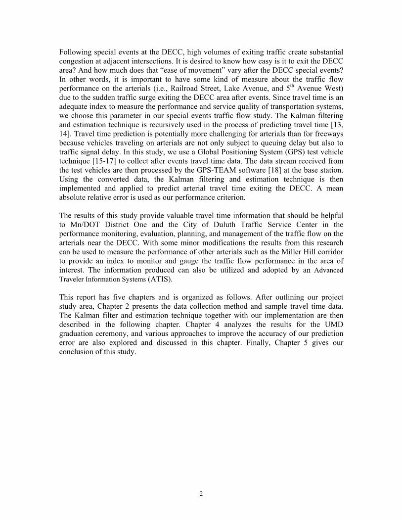
The GPS Test Vehicle Technique The test vehicle technique has been used for travel time data collection since the late 1920s. Traditionally, this technique has involved the use of a data collection vehicle within which an observer records cumulative travel time at predefined checkpoints along a travel route. This information is then converted to travel time, speed, and delay for each segment along the survey route. There are several different methods for performing this type of data collection, depending on the instrumentation used in the vehicle and the driving instructions given to the driver. Since these vehicles are instrumented and then sent into the field for travel time data collection, they are sometimes referred to as “active” test vehicles. Conversely, “passive” ITS probe vehicles are vehicles that are already in the traffic stream for purposes other than data collection [16]. Historically, the manual method has been the most commonly used travel time data collection technique. This method requires a driver and a passenger to be in the test vehicle. The driver operates the test vehicle while the passenger records time information at predefined checkpoints. GPS has become the most recent technology to be used for travel time data collection (e.g., [17, 18]). Using this technique, a GPS receiver is connected to a portable computer and collects the latitude and longitude information that enables tracking of the test vehicle. The GPS was originally developed by the Department of Defense for the tracking of military ships, aircraft, and ground vehicles. Signals, sent from the 24 satellites orbiting the earth at 20,120 km (12,500 mi), can be used to monitor location, direction, and speed anywhere in the world. An excellent book detailing the basic principle and applications of GPS can be found in [19]. A consumer market has quickly developed for many civil, commercial, and research applications of GPS technology including recreational (e.g., backpacking, boating), maritime shipping, international air traffic management, and vehicle navigation. The location and navigation advantages of GPS have found many uses in the transportation profession. Figure 2.2 illustrates the equipment needs for GPS travel time data collection [16]. The test vehicle is shown at the top of the figure with the GPS and Differential GPS (DGPS) antennas mounted on the roof of the vehicle. The DGPS antenna is connected to the differential correction receiver while the GPS antenna is connected to the GPS receiver. The differential correction data is then transferred to the GPS receiver. The GPS receiver uses the differential correction data to correct incoming signals and then the corrected information is output to the in-vehicle laptop. The laptop stores the data at predefined time intervals as the vehicle travels down the roadway. When the travel time run is completed, the laptop information is downloaded to a data storage computer. In this project, both the manual and GPS test vehicle methods are used to collect travel time data. In the manual approach, we used stopwatches and clipboards. Stopwatches provide the second increment of time for travel time data collection. The data collected by these two methods are cross verified in order to improve the data reliability and robustness. The following section briefly describes the equipment used together with the GPS-TEAM software.

5

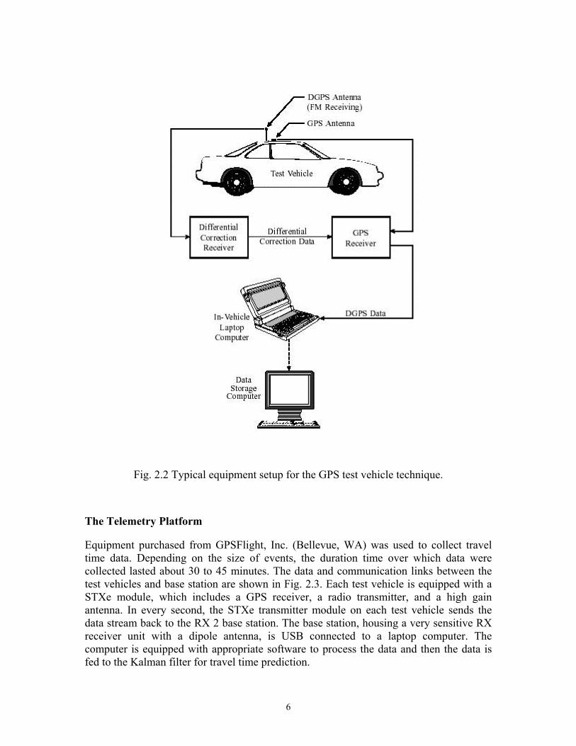
Fig. 2.2 Typical equipment setup for the GPS test vehicle technique.

The Telemetry Platform Equipment purchased from GPSFlight, Inc. (Bellevue, WA) was used to collect travel time data. Depending on the size of events, the duration time over which data were collected lasted about 30 to 45 minutes. The data and communication links between the test vehicles and base station are shown in Fig. 2.3. Each test vehicle is equipped with a STXe module, which includes a GPS receiver, a radio transmitter, and a high gain antenna. In every second, the STXe transmitter module on each test vehicle sends the data stream back to the RX 2 base station. The base station, housing a very sensitive RX receiver unit with a dipole antenna, is USB connected to a laptop computer. The computer is equipped with appropriate software to process the data and then the data is fed to the Kalman filter for travel time prediction.

6

Fig. 2.3 The GPS test vehicle travel time data collection.

The telemetry platform consists of the following components:

• The TracID Hardware Platform The GPS-integrated telemetry unit is low-cost, micro-sized with an onboard telemetry “TracID” CPU. The receiver base station is used to pick up the signals and display the results on a PC in “plug-and play” fashion. The transmitter we used is the STXe module with TracID, which is built around patent-pending proprietary firmware algorithms enabling multiple devices to submit information across a wide-spread, dispersed network without collision, and keep very accurate synchronization among all units. The STXe transmitter module is shown in Fig. 2.4. Figure 2.5 shows the module mounted on a test vehicle. The RX-B2 receiver module is shown in Fig. 2.6 and Fig. 2.7 shows the mobile base station with a Windows XP based laptop computer. In addition to data conversion, the laptop will process incoming data and then compute and generate predicted travel time via the implemented Kalman filter model.

7

Fig. 2.4 The STXe transmitter module with an antenna.

Fig. 2.5 The STXe transmitter module mounted on a test vehicle.

8

Fig. 2.6 The RX-Base 2 module with a 900 MHz magnetic mount antenna.

• SWARM and TracID A network of units communicating in this fashion is known as a Synchronized Wide Area Remote Modules (SWARM) Network. The SWARM protocol enables compressed packed data transmissions including GPS and other data, and allows individual identification by TracID. The SWARM can support more than 46,000 units with a maximum of 10 units per second reporting per network. A total of seven independent networks are possible per geographic area. Each of these seven networks operate independent from each other, so up to 7 different networks can operate in the same location without interfering with each other as well.

• GPSFlight Radio Link GPSFlight radio link supports 900 MHz spread spectrum communication at speeds of 9600 bits per second. With the compression on the data stream through TracID, the throughput is typically about 8 times that of the National Marine Electronics Association (NMEA) standard telemetry (i.e., 76.8 kb). From a range perspective, the 900 MHz products have demonstrated real-time links of over 30 miles line of sight using 2dB omni directional antennas. For non line of sight, the range is 1200 to 2000 ft (Please refer to the web site http://www.gpsflight.com for details).

9

Fig. 2.7 The mobile base station with the receiver unit.

To improve the signal reception, we upgraded (i) the antenna for each transmitter module from its original built-in 1 dB antenna to a MMCX connected 2dB gain 6” half-wavelength antenna (shown in Fig. 2.8) and (ii) the antenna for the receiver from a 2 dB RPSMA antenna to the HyperGain® HG903MGU 3.5 dB magnetic vehicle mount omni antenna (shown in Figs. 2.6 and 2.9). Note that the HyperGain mobile antenna was manufactured by HyperLink Technologies, Inc. in Boca Raton, FL. For details about this antenna, please refer to http://www.hyperlinktechnologies.com . We found that as a result of this upgrade, the average data reception rate improved from 85% to 95%.

10

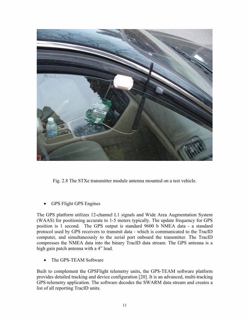
Fig. 2.8 The STXe transmitter module antenna mounted on a test vehicle.

• GPS Flight GPS Engines

The GPS platform utilizes 12-channel L1 signals and Wide Area Augmentation System (WAAS) for positioning accurate to 1-5 meters typically. The update frequency for GPS position is 1 second. The GPS output is standard 9600 b NMEA data - a standard protocol used by GPS receivers to transmit data - which is communicated to the TracID computer, and simultaneously to the serial port onboard the transmitter. The TracID compresses the NMEA data into the binary TracID data stream. The GPS antenna is a high gain patch antenna with a 4” lead.

• The GPS-TEAM Software Built to complement the GPSFlight telemetry units, the GPS-TEAM software platform provides detailed tracking and device configuration [20]. It is an advanced, multi-tracking GPS-telemetry application. The software decodes the SWARM data stream and creates a list of all reporting TracID units.

11

Fig. 2.9 The transmitter antenna magnetically mounted on the roof of a test vehicle.

Some of the important features of the GPS-TEAM software are:

1. Programming the GPS, radio, and TracID CPU 2. Display of all reporting TracID units in a network 3. Map library which enables any bit-mapped map to be used for plotting in real

time 4. TracID statistics table which lists continually updating speed, position, heading

information as well as maximums attained 5. Events window which lists the time, location, and altitude of any event, similar to

a waypoint 6. Altitude plot which shows all TracIDs in an altitude window at the same time 7. Setting of “Ground Zero" for horizontal and vertical starting position

A snapshot of the GPS-TEAM displayed on the laptop at the base station is given in Fig. 2.11. Note that in this figure the lower right window shows the path of the test vehicles traveling along Railroad Street and Lake Avenue North, while the lower left window shows the real time data stream received from all three test vehicles.

12

Fig. 2.10 A snapshot of the GPS-TEAM software.

Sample Travel Time Data The travel time data of a representative special event are explained and shown in this section. In Fig. 2.1, we divide the arterial/path from Railroad Street exiting the DECC to the intersection of Lake Avenue North & I-35 into three sections with the signalized intersections as our checkpoints. The 1st section is from the DECC exit on Railroad Street to the intersection of Railroad Street and Lake Avenue South. The 2nd section is from the intersection of Railroad Street and Lake Avenue South to the intersection of Railroad Street and Canal Park Drive and the 3rd one is from the intersection of Railroad Street and Canal Park Drive to the intersection of I-35 and Lake Avenue North. A simplified map labeling these sections is shown in Fig. 2.11. Travel time includes the vehicle’s travel time plus its wait time (i.e., the duration time the vehicle stopped by traffic lights). Currently, the traffic signal cycle length run at the DECC area during the weekdays is 80 seconds (except the time period from 3:30 pm to 7:00 am where 100 seconds is used). The cycle length is the total time to complete one sequence of signalization around an intersection. A traffic signal phase (or split) is the part of the cycle given to an individual movement, or combination of non-conflicting movements during one or more intervals. An interval is a portion of the cycle during which the signal indications do not change. In general, there are eight possible phases at

13

every intersection, although all of them are not always used. For example, the traffic signal at the intersection of Railroad Street and Lake Avenue South uses a 5-phase timing sequence, while the other two intersections in Fig. 2.11 use a 6-phase timing plan. For details about the signal timing at the DECC, please refer to [21].

Fig. 2.11 The road sections divided by the signalized intersections.

Using the GPS test vehicle technique, the total and section travel times were collected for DECC special events over a 7-month time period (i.e., November 2003 – May 2004). These special events include the UMD Men’s and Women’s hockey games, concerts, the Shrine circus, and the UMD and College of St. Scholastica graduation ceremonies. Three test vehicles were used to report travel time data. These vehicles were sent to the field and followed the pre-specified path in Fig. 2.11. The departure time interval was set to be either 3 or 5 minutes (see Chapter 4 for details). That is, each test vehicle left the DECC exit on Railroad Street 3 or 5 minutes later than the previous vehicle. After completing the journey, each vehicle returned back to the original point and joined the current traffic to start over again. The entire process continued until the traffic near the DECC was back to normal. Note that the departure time interval is actually the time step for the Kalman filter to predict the next travel time. The complete travel time data together with the project related information can be found in our web site http://www.d.umn.edu/~wwwmndot. The sample travel time data for the UMD graduation ceremony on May 15, 2004 is shown in Fig. 2.12.

14

Fig. 2.12 Measured travel times over the three road sections.

There are four curves in Fig. 2.12. The blue curve (labeled “Total”) represents the total travel time (or path travel time) from exiting the DECC till entering the intersection of I-35 and Lake Avenue North. The travel times associated with the road section 1, 2, and 3 (i.e., the link travel times) are shown with label “section 1” (red), “section 2” (yellow), and “section 3” (pink), respectively. The travel time includes wait time and it is the averaged travel time measured by the three test vehicles. The traffic following this particular event lasted about 45 minutes. The maximum path travel time was about 18.25 minutes. As can be seen from the above figure, during the peak most of the travel time elapses in section 1. This is because the distance of section 1 is much longer than that of the other two. In general, the test vehicles have to wait at intersection 1 for several signal cycles instead of only one cycle at intersections 2 and 3. In sections 2 and 3 the length of the vehicle waiting queue is limited by the relatively shorter distance of both sections. Therefore, the link travel times associated with these two sections are relatively constant and have shorter wait time. Experience showed that under the current signal timing, our test vehicles can pass intersections 2 and 3 with relatively smaller delay.

15

CHAPTER 3

KALMAN FILTERING

Travel time estimation and prediction has been an important research topic for decades. Although research on travel time estimation for freeways is very rich, research on arterial travel time estimation is quite limited. Prediction of travel time is potentially more challenging for arterials than for freeways because vehicles traveling on arterials are subject not only to queuing delay but also to signal delays as well as delays caused by vehicles entering from the cross streets. Lin et al. formulated the arterial travel time prediction problem into a Markov chain model with a one-step transition matrix [22]. However, their model has some inherent limitations. One of them is that the nominal delay used in the formulation is based on the existing delay formula for intersections. It is well known that many existing delay formula perform poorly for over-saturated intersections. Sisiopiku et al. studied to improve the performance of arterial travel time estimation by examining the use of detector output from simulation and field studies [4, 23]. But their method is unable to predict travel time when the queues extend over the detector location. Artificial neural networks (ANNs) have been used for prediction but they need a long time to learn the training data and the determination of the optimum architecture is also a trial-and-error procedure. The Kalman filter algorithm was also used by Okutani and Stephanedes to predict traffic volume in urban network [24]. The advantage of using the Kalman filter is that it can update the parameter to make the predictor reflect the traffic fluctuation quickly. Compared with the Kalman filter algorithm, predicting travel time with ANNs may be less accurate if the future traffic patterns are not in the training samples. In this study, the Kalman filtering and estimation technique [13-15, 26] is used to predict travel time following DECC special events. Background The Kalman filter has been used extensively in many areas (e.g., navigation, guidance and control) with lots of practical applications reported in the literature (e.g., [13, 15, 19]). Its basic function is to provide estimates of the current state of the system. But it also serves as the basis for predicting future values of prescribed variables or for improving estimates of variables at earlier times. Since the introduction of the Kalman filter and its initial applications in the early 1960’s, many theoretical papers have been stimulated by problems encountered in applying the Kalman filter to practical problems. Due to the advances in digital computing, the Kalman filter has been the subject of extensive research and applications, particularly in the area of autonomous and assisted navigation. Recently, it has also been used in travel time estimation problems [25-27]. The Kalman filter basically is a set of mathematical equations that provides an efficient computational (recursive) means to estimate the state of a process, in a way that minimizes the mean of the squared error. The filter is very powerful in several aspects: it supports estimations of past, present, and even future states, and it can do so even when the precise nature of the modeled system is unknown. It tells how the past values of the

16

input should be weighted in order to determine the present value of the output, that is, the optimal estimate. The two main features of the Kalman formulation and solution of the problem are (1) vector modeling of the random processes under consideration, and (2) recursive processing of the noisy measurement (input) data. By providing a way of formulating the least squares filtering problem using state-space methods, the Kalman filter can solve many discrete-time, multi-input multi-output problems. The Filtering Process In the following, we briefly summarize the main results of the Kalman filter. Assume that the random process to be estimated can be modeled as

kkkk wxx +=+ φ1 (1) where

)1( ×= nxk state vector at time k )( nnk ×=φ state transition matrix relating xk to xk+1 without a forcing function )1( ×= nwk vector representing a white noise sequence

The observation (measurement) of the process is assumed to be

kkkk vxHz += (2) where

)1( ×= mzk measurement vector at time k matrix giving the connection between the measurement and the state )( nmH k ×=

vector at time k (under noise-free condition) )v measurement error 1( ×= mk

The covariance matrices for the noise sequences {wk} and {vk}are given by Qk and Rk, respectively. And Qk and Rk have the following properties: (a) E[wkiwi

T] = Qk for k = i and 0 for k ≠ i; (b) E[vkvj

T] = Rk for k =j and 0 for k ≠ j, where the superscript T means the transpose and the symbol E[·] represents the expected value. We assume that {vk} is a white sequence and is also uncorrelated with {wk}, that is, E[wkivi

T] = 0 for all k and i. Assume that we have an initial estimate of the process at time k, and that this estimate is based on what is known about the process prior to k. This prior estimate will be denoted as where “hat” denotes estimate and the superscript “-” is a reminder that this is the best estimate prior to assimilating the measurement at k.

−kx̂

Now, define the estimation error to be

17

(3)

−− −= kkk xxe ˆ

and the associated error covariance matrix

(4) ])ˆ)(ˆ[(][ T

kkkkT

kkk xxxxEeeEP −−−−− −−==

Then, a linear blending of the noisy measurement and the prior estimate is chosen to be

)ˆ(ˆˆ −− −+= kkkkkk xHzKxx (5) where is the updated estimate and Kkx̂ k is the blending factor. Note that the justification of the special form of Eq. (5) can be found in [14]. The optimal estimation problem is to find a particular Kk to minimize the performance criterion chosen to be the diagonal elements of the error covariance matrix Pk (to be given in Eq. (7)). Note that these diagonal terms represent the estimation error variances for the elements of xk being estimated. There are several ways to solve this optimization problem (e.g., [13-15]). The optimal Kk, called the Kalman gain, is found to

(6) 1)( −−− += kTkkk

Tkkk RHPHHPK

which minimizes the mean-square estimation error. In addition, the relationship between Pk and can be further expressed as [14] −

kP

(7) −−= kkkk PHKIP )(

Since

(8) kkk xx ˆˆ 1 φ=−+

we can rewrite the expression for as −+1kP

(9) kTkkkk QPP +=−

+ φφ1

Note that Eq. (9) can be derived using Eqs. (3) and (4) with the index k replaced by k+1 together with Eqs. (1) and (8). With the results given above, the equations and the sequence of computational steps can now be summarized in Fig 3.1.

18

Fig. 3.1 The Kalman filter loop.

Implementation The technique in the previous section is applied and used to predict special events travel time from the DECC exit on Railroad Street to I-35 on Lake Avenue North. The problem is formulated as a recursive procedure using the results of the current step to obtain the results for the next step. Both historic data and real-time data are used in our prediction process which can be summarized as follows. Assume that our prediction process can be modeled as Eq. (1). That is,

kkkk wxx +=+ φ1 (10)

where the state variable xk is the travel time to be predicted at time k, kφ is the state transition parameter relating xk to xk+1, and wk is a zero mean Gaussian noise sequence with covariance Qk. That is, , where )(][ jiQwwE i

Tji −= δ )( ji −δ is the δ function which

equals to 1 for i = j and 0 for i ≠ j. Note that, in general, xk and wk are in vector form with the same dimension. In this application, xk and wk are scalar, and historic data are used to obtain kφ , which describes the time dependent relationship between the travel times in any two consecutive time intervals.

19

Since no additional traffic parameter other than travel time is involved, the measurement/observation equation associated with the state variable xk is modeled by Eq. (2) and is repeated below

kkkk vxHz += (11)

where zk represents the observation, i.e., the average of the travel times reported by the test vehicles at time k. The parameter Hk correlates the functional connection between xk and zk (in our case, Hk =1) and the measurement noise {vk} is a Gaussian sequence with zero mean and covariance Rk. Again, assume that {wk} and {vk} are uncorrelated (i.e.,

for all i and j). Furthermore, let the prediction error and P0][ =TjivwE −− −= kkk xxe ˆ k be

the error covariance at time k. Then, our travel time prediction, based on the minimization of the trace of Pk, can be summarized as follows:

Step 1: Initialization Set k = 0 and let 00 ˆ][ xxE = and 0

20 ][ PeE =

Step 2: Extrapolation

State estimate extrapolation: kkk xx ˆˆ 1 φ=−+

Error covariance extrapolation: kTkkkk QPP +=−

+ φφ1

Step 3: Kalman gain calculation

1)( −−− += kTkkk

Tkkk RHPHHPK (Hk =1)

Step 4: Update

State estimate update: )ˆ(ˆˆ −− −+= kkkkkk xHzKxx Error covariance update: −−= kkkk PHKIP )(

Step 5: Let k = k + 1 and go to Step 2 until the preset time period ends.

Computer Program Based on the implementation steps shown in the previous section, a computer program has been developed for recognizing TracID binary data stream and implementing Kalman filtering online. The input of the program is historic (average) travel time and TracID binary data stream sent by GPS-TEAM in real-time. The output generated by the program is the synchronously predicted travel time. The TracID binary data stream is sent from the STXe transmitters installed in test vehicles to GPS-TEAM every second. The computer program transfers these data stream into recognized position (i.e., longitude and latitude) and time information. When the test vehicles pass the pre-defined start and end points, the time is recorded and travel time is computed. With historic data, these travel

20

time data are fed into the Kalman filter to get the predicted travel time in the next time interval. The program runs recursively until the traffic congestion is over. Figure 3.2 shows the flow chart of our implemented program. The complete program listing is available upon request.

21

Fig. 3.2 The flowchart of the implemented computer program.

22

CHAPTER 4

RESULTS OF TRAVEL TIME PREDICTION The travel time prediction results for the DECC special events were conducted and investigated. In this chapter, we focus on a case study of the UMD graduation ceremony. This special event is selected due to its relatively large traffic volume as compared with other events. Very similar results were found for other events. We first present and compare the path and link travel time prediction results. The main criteria used for the error analysis is Mean Absolute Relative Error (MARE). A lower MARE indicates a better result. The effect of reducing the prediction time interval is then studied. Furthermore, the methods of using the rate of change of historic data (i.e. the slope information) and the data interpolation technique are also explored to improve the accuracy of our travel time prediction. Mean Absolute Relative Error (MARE) Based on Fig. 2.12, the comparison of the predicted and measured path travel times is shown in Fig. 4.1, where the predicted travel time at each time instant is compared with the corresponding observed travel time.

Fig. 4.1 Comparison of the predicted and observed travel times.

23

The predicted travel time at current time instant is basically determined by both the observed and predicted travel times at the previous time instants. A larger prediction error occurred if there is a sudden dramatic change (increase or decrease) of actual travel time. Overall speaking, the predicted travel time follows the observed one. We found that the average error would be smaller if the duration time of traffic congestion lasts longer. To quantify the prediction error, we use a mean absolute relative error (MARE) as our performance criterion, which is defines as follows

^

1| |

100%

ni i

i i

x xxMARE

n=

−

= ×∑

(12)

where ix is the actual value and ^

ix represents the predicted value. The prediction error, expressed in MARE, is shown in Table 4.1.

Special Event &

Date

T (min)

N

MARE (%)

UMD

Commencement May 15, 2004

3.0

15

17.61

Table 4.1 The prediction error for the UMD graduation ceremony. In Table 4.1, the prediction time interval T is set to be 3 minutes and the number of intervals N for this particular event is 15. That is, the departure time among the three test vehicles exiting the DECC is 3 minutes apart and, thus, the computer program predicts the travel time every 3 minutes. The traffic event lasted about 45 minutes and there are 15 iterations over the entire time period we studied. The averaged absolute relative error is about 17.61 %, a reasonably good given the fact of many uncertainties (e.g., weather, traffic condition, signal timing) associated with such an event. The error index, MARE, gives us an indication of how close the predicted travel time from the actual one. Note that the GPS signals are received from the test vehicles every second while the travel time prediction is performed every 3 minutes. For a given special event, to reduce the prediction time interval we need to increase the number of test vehicles used in our data collection.

24

Link Travel Time Prediction The prediction error comparison for the three road sections in Fig. 2.11 is given in Table 4.2. Of the three road sections, the section 3 generates a relatively small error. This is due to the smaller variance of the link travel time we observed in section 3. As mentioned, a large sudden change in travel time incurs a larger prediction error. Overall, the MARE of all three sections is roughly within the same range. Figure 4.2 shows the predicted travel time versus the actual travel times for the three sections.

Road Section

T (min.)

N

MARE (%)

Section 1

3.0

15

24.98

Section 2

3.0

15

25.17

Section 3

3.0

15

21.25

Table 4.2 Error performance comparison for the three road sections.

25

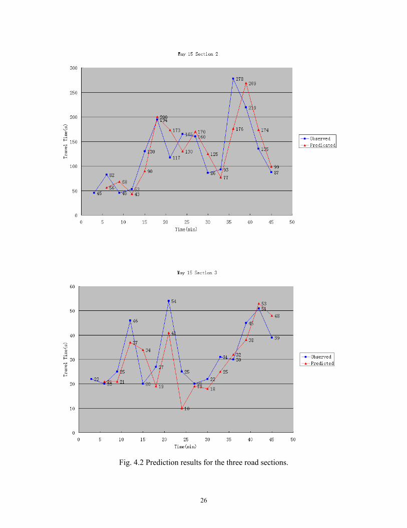
Fig. 4.2 Prediction results for the three road sections.

26

Effect of Prediction Time Interval on Error The prediction time interval (i.e., T) is a time step within which data is collected for predicting travel time in the next time step. The entire duration time for a prediction process depends on the level of traffic congestion and the number of test vehicles used over time. Both 3-minute and 5-minute intervals were used to evaluate the performance for the April 25 and May 22 concerts with the results given in Table 4.3. Form Table 4.3, apparently the prediction using a 3-minute interval seems better with the error reduced from the original 33.44 % to 21.20 %. Since the duration time of traffic congestion for similar events is about the same, reducing the prediction time interval (T) means increasing the number of intervals (N) and, thus, the number of iterations. In general, the shorter T is, the better the prediction result will be.

Date and Special

Events

T (min)

N

MARE (%)

April 25 Concert

5.0

6

33.44

May 22 Concert

3.0

9

21.20

Table 4.3 Error performance comparison for T = 3 and 5 minutes.

Data Interpolation Since the number of test vehicles is fixed, to improve the error we increase the number of prediction time interval (i.e., N) by using a data interpolation technique. That is, we artificially create a data point between any two existing consecutive data points by averaging. In other words, the values of interpolated data points are calculated by averaging the values of consecutive data points between which data points are interpolated. Besides the one-point data interpolation, the interpolation with two new data points generated between any two original, consecutive ones is also considered. The results by interpolating one- and two-data points are given and compared in Table 4.4. From this table, we see that the MARE is reduced from the original 17.61 % to 7.68 % and 4.40 % for one- and two-point data interpolation, respectively. Apparently, the prediction error improves dramatically after the interpolation is used. With the increased

27

number of data points, the prediction is less likely to be affected by the sudden increase or decrease of the actual travel time. Obviously, the more data points are used, the better the error performance will be. Implicitly, this further implies that the travel time prediction results can be improved if more test vehicles are used. Of course, this will also increase the entire operation cost (equipment, staff, etc.) in the data collection work.

Date Interpolation

T (min.)

N

MARE (%)

Original

3.0

15

17.61

1 - point data

interpolation

1.5

29

7.68

2 - point data

interpolation

1.0

43

4.40

Table 4.4 Error performance comparison with interpolated data points. With Fig. 4.1 as the base line, Figure 4.3 shows the original prediction result over the 45-minute time period, together with the ones using the data interpolation technique. Comparing these three figures, it is clear that the predicted travel time (the red curve) is improved as the interpolation method is used, and it has a much better match to the observed travel time (the blue curve) when the two-point interpolation is used.

28

(Original)

29

Fig. 4.3 Prediction results with data interpolation.

Effect of Using Historic Data on Prediction Error Based on the traffic volume involved and similarity observed, we categorized the DECC special events into three types: UMD Men’s hockey games, graduate ceremonies, and concerts (including all other events such as circus). Historic travel time data were averaged and used to adjust the prediction technique. Since the prediction error is mostly caused by sudden increase and decrease of travel time, the predicted travel time generated by the Kalman filter is modified by incorporating the available information, i.e., the rate of change of historic data. Let hn be the historic travel time observed at time n, xn be the predicted travel time generated by the Kalman filter, and yn be the predicted travel time adjusted using the historic data, then yn

is calculated as 2/)]([ 11 −− −++= nnnnn hhyxy . This method was tested on several occasions. However, we found that the results can be improved only when the actual travel time data are similar to the historic data. The effect of using this information for the April 25 event (Shrine circus) is shown in Fig. 4.4. From this figure, we see that the discrepancy between the actual and predicted travel times is reduced after the above adjustment was made. Additionally, a combined method of using both the interpolation technique and historic data is summarized in Table 4.5. Using the two-point data interpolation with the slope information included, the prediction error is reduced to 17.11 % as compared with the original 33.44 %.

30

Fig. 4.4 Effect of the usage of historic data.

Methods

T (min.)

N

MARE (%)

Original

5.0

6

33.44

Slope adjusted

5.0

6

27.57

Slope adjusted

+ 1-point Interpolation

2.5

11

24.08

Slope Adjusted

+ 2-point Interpolation

1.67

16

17.11

Table 4.5 Error performance comparison with historic data and interpolated points.

31

Effect of Noise Variance on Prediction Error The effect of varying the parameters Qk (i.e., the variance of the process noise) and Rk (i.e., the variance of the measurement noise) on the prediction error is also studied. Different values of Qk and Rk are used to compare the MARE index, and the results for the UMD graduation ceremony are list in Table 4.6.

Rk/Qk 25 50 100 1,000 10,000 100,000

1 0.232 0.120 0.061 0.006 0.001 0.000

10 1.661 0.971 0.537 0.061 0.006 0.001

100 5.488 4.281 3.031 0.537 0.061 0.006

1,000 8.257 7.610 6.835 3.031 0.537 0.061

10,000 9.337 9.198 8.900 6.835 3.031 0.537

21,394 9.390 9.343 9.219 7.675 4.404 1.025

100,000 9.485 9.447 9.405 8.900 6.835 3.031

Table 4.6 MARE using different measure error variance and noise sequence variance.

Generally, MARE drops when the measurement error variance R decreases and the process noise variance Q increases. Note that in our study, the measurement error variance used is the averaged variance of the historic travel time, which is 21,394 and the noise sequence variance Q we choose is 10,000.

32

CHAPTER 5

CONCLUSION Following special events at the DECC (e.g., conventions, concerts, graduation ceremonies, etc.), high volumes of traffic exiting the DECC create substantial congestion at adjacent intersections. This report focuses on the mobility study and travel time prediction on the arterials in the adjacent area near the DECC. Travel time is used as a parameter to measure the performance due to the following reasons: (a) it is the most common way that users measure the quality of their trip; (b) it is a variable that can be directly measured; (c) it is a simple measure to use for traffic monitoring. This information is needed to identify and assess operational problems along highway facilities, and it is also necessary in traffic signal timing control coordination, as input to traffic assignment algorithms, and in economic studies, etc. Therefore, travel time data have always been of interest to traveler information researchers, planners, and public agencies as a key measure in performance monitoring of traffic systems. The travel time data, collected via the GPS test vehicle technique, are used to measure the performance. Using the STXe and RX-Base 2 transmitter/receiver modules, three test vehicles were sent to the field to collect data. The data collection was conducted over a seven-month period. Based on the historic and real-time data, a recursive, discrete-time Kalman filter is used. The predicted travel time at current time instant is determined by the observed and predicted travel times at the previous time instants and the entire process is recursively performed in discrete time. The filtering and estimation method is briefly introduced before the flow chart to implement the real-time prediction is presented. Finally, an assessment of the performance and its effectiveness at the test site are investigated. To quantify the prediction error, we use a mean absolute relative error (MARE) as our performance criterion. The results for the UMD graduation ceremony are analyzed and various approaches to improve the accuracy of our prediction error is also explored and discussed. The possible methods include: (a) reducing the prediction time interval; (b) using the data interpolation technique; and (c) using the rate of change of historic data. The effects of changing the noise parameters on the prediction error are also studied. The results from this research will help Mn/DOT District 1 and the City of Duluth Traffic Service Center manage the traffic flow following special events at the DECC more efficiently. It will provide a valuable assessment tool to address these questions such as how easy is it to move around and exit the area and how much does that “ease of movement” vary after the DECC special events. The results of this research can also provide valuable travel time information to the motorists when making their route choices. In addition, the travel time prediction generated from this research can be easily applied to arterials such as the Miller Hill corridor (Central Entrance – Miller Trunk Highway) to provide an index to monitor and gauge the traffic system performance in the area of interest. This should be helpful to Mn/DOT District One in the performance monitoring, evaluation, planning, and management of the arterial traffic flow in the Duluth area.

33

REFERENCES

[1] H. Al-Deek, M. D’Angelo, and M. Wang, “Travel Time Prediction with Non-linear Time Series,” Proceedings of the 5th ASCE International Conference on Applications of Advanced Technologies in Transportation, pp. 317-324, 1998.

[2] M. S. Ahmed and A. R. Cook, “Analysis of Freeway Traffic Time Series Data by

Using Box-Jenkins Techniques,” Transportation Research Record 722, pp. 1-9, 1979. [3] L. Rilett and D. Park, “Direct Forecasting of Freeway Corridor Travel Times Using

Spectral Basis Neural Networks,’’ Transportation Research Record 1617, pp. 163-170, 1999.

[4] P. V. Palacharla and P. C. Nelson, “Application of Fuzzy Logic and Neural Networks

for Dynamic Travel Time Estimation,” International Transactions in Operational Research, vol. 6, pp. 145-160, 1999.

[5] V. P. Sisiopiku, N. M. Rouphail, and A. Santiago, “Analysis of Correlation Between

Arterial Travel Time and Detector Data From Simulation and Field Studies,” Transportation Research Record 1457, pp. 166-173, 1994.

[6] D. J. Dailey, “Travel-Time Estimation Using Cross-Correlation Techniques,”

Transportation Research, Part B, vol. 27, pp. 97-107, 1993. [7] I. Okutani and Y. J. Stephanedes, “Dynamic Prediction of Traffic Volume Through

Kalman Filtering Theory,” Transportation Research, Part B, vol. 18, pp. 1-11, 1984. [8] B. L. Smith, “Forecasting Freeway Traffic Flow for Intelligent Transportation

Systems Application,” Transportation Research, Part A, vol. 31, pp. 61, 1997. [9] H. Suzuki, T. Nakatsuji, Y. Tanaboriboon, and K. Takahashi, “A Neural-Kalman

Filter for Dynamic Estimation of Orgin-Destination Travel Time and Flow on a Long Freeway Corridor,” Transportation Research Record 1739, pp. 67-75, 2000.

[10] M. Chen and S. Chein, “Dynamic Freeway Travel Time Prediction Using Probe Vehicle Data: Link-based vs. Path-based,” Transportation Research Record, in press. [11] I. Christiansen and L. Hauer, “Probe Vehicles for Travel Time,” Traffic Technology International, August/September issue, pp. 41-44, 1996.

[12] J. You and T. J. Kim, “Development and Evaluation of a Hybrid Travel Time Forecasting Model,” Transportation Research, Part C, vol. 8, pp.231-256, 2000.

[13] H. W. Sorenson., Kalman Filtering: Theory and Application, IEEE Press, New York, 1985.

34

[14] R. G. Brown and Y. C. Hwang, Introduction to Random Signals and Applied Kalman Filtering, 3rd Edition, John Wiley & Sons, New York, 1997. [15] P. Zarchan and H. Musoff, Fundamentals of Kalman Filtering and Applications, American Institute of Aeronautics and Astronautics (AIAA), Reston, VA, 2000. [16] S. M. Turner, W. L. Eisele, R. J. Benz, and D. J. Holdener, Travel Time Data Collection Handbook (FHWA-PL-98-035), Texas Transportation Institute & Office of Highway Information Management, FHWA, USDOT, March 1998. [17] J. Gallagher, “Travel Time Data Collection Using GPS”, National Traffic Data Acquisition Conference, Albuquerque, New Mexico, May 1996. [18] D. Laird, “Emerging Issues in the Use of GPS for Travel Time Data Collection”, National Traffic Data Acquisition Conference, Albuquerque, New Mexico, May 1996. [19] B. W. Parkinson and J. J. Spilker, GPS: Theory and Applications, vol. I and vol.II, American Institute of Aeronautics and Astronautics (AIAA), Reston, VA, 1996. [20] GPS-Team Product Manual - Advanced Telemetry Tracking, GPSFlight, Inc. 2003. [21] J.-S. Yang, “Duluth Entertainment Convention Center (DECC) Traffic Flow Study – Traffic Data Analysis and Signal Timing Coordination”, NATSRL, Project Final Report, June 2003.

[22] W.-H. Lin, A. Kulkarni, and P. Mirchandani, “Arterial Travel Time Estimation for Advanced Traveler Information Systems,” TRB 2003 Annual Meeting.

[23] V. P. Sisiopiku and N. M. Rouphail, “Toward the Use of Detector Output for

Arterial Link Travel Time Estimation: a Literature Review,” Transportation Research Record 1457, pp. 1580165, 1994.

[24] I. Okutani and Y. J. Stephanedes, “Dynamic Prediction of Traffic Volume Through

Kalman Filtering Theory,” Transportation Research, Part B, vol. 18, pp.1-11, 1984.

[25] I. J. Chien and M. Kuchipudi., “Dynamic Travel Time Prediction with Real-time and Historical Data”, Transportation Research Board the 81st Annual Meeting, Washington D.C., January 2002. [26] S. I. Chien, X. Liu, and K. Ozbay, “Predicting Travel Times for the South Jersey Real-time Motorist Information System”, Journal of Transportation Research Board, October 2002. [27] H. Suzuki, T. Nakatsuji, Y. Tanaboriboon, and K. Takahashi, “A Neural-Kalman Filter for Dynamic Estimation of Origin-Destination (O-D) Travel Time and Flow on a Long Freeway Corridor”, Transportation Research Board 79th Annual Meeting, Washington, D. C., January, 2000.

35