CHAPTER 1

Introduction

Chapter Outline1.1 What Is Nuclear Magnetic Resonance? 1

1.2 Consequences of Nuclear Spin 2

1.3 Application of a Magnetic Field to a Nuclear Spin 4

1.4 Application of a Magnetic Field to an Ensemble of Nuclear Spins 7

1.5 Tipping the Net Magnetization Vector from Equilibrium 12

1.6 Signal Detection 13

1.7 The Chemical Shift 14

1.8 The 1-D NMR Spectrum 14

1.9 The 2-D NMR Spectrum 16

1.10 Information Content Available Using NMR Spectroscopy 18

Problems for Chapter One 19

1.1 What Is Nuclear Magnetic Resonance?

Nuclear magnetic resonance (NMR) spectroscopy is arguably the most important analytical

technique available to chemists. From its humble beginnings in 1945, the area of NMR

spectroscopy has evolved into many overlapping subdisciplines. Luminaries have been

awarded several recent Nobel prizes, including Richard Ernst in 1991, John Pople in 1998, and

Kurt Wuthrich in 2002.

Nuclear magnetic resonance spectroscopy is a technique wherein a sample is placed in

a homogeneous1 (constant) magnetic field, irradiated, and a magnetic signal is detected. Photon

bombardment of the sample causes nuclei in the sample to undergo transitions2 (resonance)

between their allowed spin states. In an applied magnetic field, spin states that differ

energetically are unequally populated. Perturbing the equilibrium distribution of the spin-state

population is called excitation.3 The excited nuclei emit a magnetic signal called a free

induction decay4 (FID) which we detect with analog electronics and capture digitally. The

1 Homogeneous. Constant throughout.2 Transition. The change in the spin state of one or more NMR-active nuclei.3 Excitation. The perturbation of spins from their equilibrium distribution of spin-state populations.4 Free induction decay, FID. The analog signal induced in the receiver coil of an NMR instrument caused by thexy component of the net magnetization. Sometimes the FID is also assumed to be the digital array of numberscorresponding to the FID’s amplitude as a function of time.

Organic Structure Determination Using 2-D NMR Spectroscopy.

Copyright � 2012 Elsevier Inc. All rights reserved. 1

digitized FID(s) is(are) processed computationally to (we hope) reveal meaningful things about

our sample.

Although excitation and detection may sound very complicated and esoteric, we are really just

tweaking the nuclei of atoms in our sample and getting information back. How the nuclei

behave once tweaked conveys information about the chemistry of the atoms in the molecules of

our sample.

The acronym NMR simply means that the nuclear portions of atoms are affected by magnetic

fields and undergo resonance as a result.

1.2 Consequences of Nuclear Spin

Observation of the NMR signal5 requires a sample containing atoms of a specific atomic

number and isotope, i.e., a specific nuclide such as protium, the lightest isotope of the element

hydrogen, also commonly referred to as simply a proton. A magnetically active nuclide will

have two or more allowed nuclear spin states.6 Magnetically active nuclides are also said to be

NMR-active. Table 1.1 lists several NMR-active nuclides in approximate order of their

importance to chemists.

An isotope’s NMR activity is caused by the presence of a magnetic moment7 in its nucleus.

The nuclear magnetic moment arises because the positive charge prefers not to be well located,

as described by the Heisenberg uncertainty principle (see Figure 1.1). Instead, the nuclear

charge circulates. Because the charge and mass are both inherent to the particle, the movement

of the charge imparts movement to the mass of the nucleus. The motion of all rotating masses is

Table 1.1: NMR-active nuclides.

Nuclide Element-Isotope Spin Natural Abundance (%) Frequency Relative to 1H

1H Hydrogen-1 ½ 99.985 1.0000013C Carbon-13 ½ 1.108 0.2514515N Nitrogen-15 ½ 0.37 0.1013719F Fluorine-19 ½ 100. 0.9409431P Phosphorus-31 ½ 100. 0.40481

2H (or 2D) Deuterium-2 1 0.015 0.15351

5 Signal. An electrical current containing information.6 Spin state. Syn. spin angular momentum quantum number. The projection of the magnetic moment of a spinonto the z-axis. The orientation of a component of the magnetic moment of a spin relative to the applied fieldaxis (for a spin-½ nucleus, this can be +½ or e½).

7 Magnetic moment. Avector quantity expressed in units of angular momentum that relates the torque felt by theparticle to the magnitude and direction of an externally applied magnetic field. The magnetic field associatedwith a circulating charge.

2 Chapter 1

expressed in units of angular momentum. In a nucleus, this motion is called nuclear spin.8

Imagine the motion of the nucleus as being like that of a wild animal pacing in circles in a cage.

Nuclear spin (see column three of Table 1.1) is an example of the motion associated with

zero-point energy in quantum mechanics, whose most well-known example is perhaps the

harmonic oscillator.

The small size of the nucleus dictates that the spinning of the nucleus is quantized; that is, the

quantum mechanical nature of small particles forces the spin of the NMR-active nucleus to be

quantized into only a few discrete states. Nuclear spin states are differentiated from one

another based on how much the axis of nuclear spin aligns with a reference axis (the axis of the

applied magnetic field, see Figure 1.2).

We can determine how many allowed spin states there are for a given nuclide by multiplying

the nuclear spin number (I) by 2 and adding 1. For a spin-½ nuclide, there are therefore

2 (1/2)þ 1¼ 2 allowed spin states.

In the absence of an externally applied magnetic field, the energies of the two spin states of

a spin-½ nuclide are degenerate9 (the same).

The circulation of the nuclear charge, as is expected of any circulating charge, gives rise

to a tiny magnetic field called the nuclear magnetic moment (m) e also commonly

referred to as a spin (recall that the mass puts everything into a world of angular

momentum). Magnetically active nuclei are rotating masses, each with a tiny magnet,

and these nuclear magnets interact with other magnetic fields according to Maxwell’s

equations.

Figure 1.1:The structure of an atom with the positive charge unequally distributed in the nucleus inside

the electron cloud.

8 Nuclear spin. The circular motion of the positive charge of a nucleus.9 Degenerate. Two spin states are said to be degenerate when their energies are the same.

Introduction 3

1.3 Application of a Magnetic Field to a Nuclear Spin

Placing a sample inside the NMR magnet puts the sample into a very high strength magnetic

field. Application of a magnetic field to this sample will cause the nuclear magnetic moments

of the NMR-active nuclei of the sample to become aligned either partially parallel (a spin

state) or antiparallel (b spin state) with the direction of the applied magnetic field.

Alignment of the two allowed spin states for a spin-½ nucleus is analogous to the alignment of

a compass needle with the Earth’s magnetic field. A point of departure from this analogy comes

when we consider that nearly half of the nuclear magnetic moments in our sample line up with

their z-component opposed to the direction of the magnetic field lines we apply (applied

field).10 A second point of departure from the compass analogy is due to the small size of the

nucleus and the Heisenberg uncertainty principle (again!). The nuclear magnetic moment

cannot align itself exactly with the applied field. Instead, only part of the nuclear magnetic

Figure 1.2:Application of an external magnetic field forces the spin-½ nucleus to adopt either the spin-up (a) or

spin-down (b) state.

10 Applied field, B0. Syn. applied magnetic field. The area of nearly constant magnetic flux in which the sampleresides when it is inside the probe which is, in turn, inside the bore tube of the magnet.

4 Chapter 1

moment (half of it) can align with the field. If the nuclear magnetic moment were to align

exactly with the applied field axis, then we would essentially know too much, which

nature does not allow. The Heisenberg uncertainty principle mathematically forbids the

attainment of this level of knowledge. This limitation rankled Albert Einstein, prompting him

to quip “God does not play dice with the universe.” At this level, we accept the stochastic

nature of spins.

The energies of the parallel and antiparallel spin states of a spin-½ nucleus diverge linearly

with increasing magnetic field. This is the Zeeman effect11 (see Figure 1.3). At a given

magnetic field strength, each NMR-active nuclide exhibits a unique energy difference between

its spin states. Hydrogen has the second greatest slope for the energy divergence (second only

to its rare isotopic cousin, tritium, 3H or 3T). This slope is expressed through the gyromagnetic

ratio,12 g, which is a unique constant for each NMR-active nuclide. The gyromagnetic ratio

tells how many rotations per second (gyrations) we get per unit of applied magnetic field

(hence the name, gyromagnetic). Equation 1.1 shows how the energy gap between states (DE)

of a spin-½ nucleus varies with the strength of the applied magnetic field B0 (in tesla). By

necessity, the units of g are joules per tesla:

DE ¼ gB0 (1.1)

Figure 1.3:Zeeman energy diagram showing how the energies of the two allowed spin states for the spin-½

nucleus diverge with increasing applied magnetic field strength.

11 Zeeman effect. The linear divergence of the energies of the allowed spin states of an NMR-active nucleus asa function of applied magnetic field strength.

12 Gyromagnetic ratio, g. Syn. magnetogyric ratio. A nuclide-specific proportionality constant relating howfast spins will precess (in radians $ sece1) per unit of applied magnetic field (in T).

Introduction 5

To induce transitions between the allowed spin states of an NMR-active nucleus, photons with

their energy tuned to the gap between the two spin states must be applied (Equation 1.2):

DE ¼ hn ¼ Zu (1.2)

where h is Planck’s constant in joule seconds, n is the frequency in events per second, Z (“h bar”)

is Planck’s constant divided by 2p, and u is the angular frequency in radians per second.

From Equations 1.1 and 1.2 we can calculate the NMR frequency of any NMR-active nuclide

on the basis of the strength of the applied magnetic field alone (Equations 1.3a and 1.3b). In

practice, the gyromagnetic ratio we look up may already have the factor of Planck’s constant

included; thus, the units of g may be in radians per tesla per second. For hydrogen, g is

2.675� 108 radians/tesla/second (radians are used because the radian is a ‘natural’ unit for

oscillations and rotations), so the frequency is

v ¼ �gB0=h (1.3a)

or

u ¼ �gB0=Z (1.3b)

Positive rotation is defined as being counter-clockwise. To calculate NMR frequency correctly,

it is important we make sure our units are consistent. For a magnetic field strength of

11.74 tesla (117,400 gauss), the NMR frequency for hydrogen is

v ¼ 2:675 � 108 radians=tesla=second� 11:74 tesla=2p radians=cycle

¼ 4:998� 108 cycles=second ¼ 500 MHz(1.4)

Thus, an NMR instrument13 operating at a frequency of 500 MHz requires an 11.74 tesla

magnet. Each spin experiences a torque from the applied magnetic field. The torque applied to

an individual nuclear magnetic moment can be calculated by using the right-hand rule because

it involves the mathematical operation called the cross product.14 Because a spin cannot

align itself exactly parallel to the applied field, it will always feel the torque from the

applied field (see Figure 1.4). Hence, the rotational axis of the spin will precess around the

applied field axis just as a top’s rotational axis precesses in the Earth’s gravitational field. The

amazing fact about the precession of the spin’s axis is that its frequency is the same as that of

a photon that can induce transitions between its spin states; that is, the precession frequency15

13 NMR instrument. A host computer, console, preamplifier, probe, cryomagnet, pneumatic plumbing, andcabling that together allow the collection of NMR data.

14 Cross product. A geometrical operation wherein two vectors will generate a third vector orthogonal(perpendicular) to both vectors. The cross product also has a particular handedness (we use the right-hand rule),so the order of how the vectors are introduced into the operation is often important.

15 Precession frequency. Syn. Larmor frequency, NMR frequency. The frequency at which a nuclear magneticmoment rotates about the axis of the applied magnetic field.

6 Chapter 1

for protons in an 11.74 tesla magnetic field is also 500 MHz! This nuclear precession

frequency is called the Larmor (or NMR) frequency.16 The Larmor frequency will become an

important concept to remember when we discuss the rotating frame of reference.

1.4 Application of a Magnetic Field to an Ensemble of Nuclear Spins

Only half of the nuclear spins align with a component of their magnetic moment parallel to an

applied magnetic field because the energy difference between the parallel and antiparallel spin

states is extremely small relative to the available thermal energy,17 kT. The omnipresent

thermal energy kT randomizes spin populations over time. This nearly complete randomization

is described by using the following variant of the Boltzmann equation:

Na=Nb ¼ expðDE=kTÞ (1.5)

In Equation 1.5, Na is the number of spins in the a (lower energy) spin state, Nb is the number

of spins in the b (higher energy) spin state, DE is the difference in energy between the a and

b spin states, k is the Boltzmann constant, and T is the temperature in degrees kelvin. Because

DE/kT is very nearly zero, both spin states are almost equally populated. In other words,

because the spin-state energy difference is much less than kT, thermal energy equalizes the

populations of the spin states. Mathematically, this equal distribution is borne out by Equation

1.5, because raising e (2.718.) to the power of almost 0 is very nearly 1; thus, showing that the

ratio of the populations of the two spin states is almost 1:1.

Figure 1.4:Diagram showing how the cross product results in a torque perpendicular to both net

magnetization vector M and applied field B0.

16 Larmor frequency. Syn. precession frequency, nuclear precession frequency, NMR frequency, rotatingframe frequency. The rate at which the xy component of a spin precesses about the axis of the appliedmagnetic field. The frequency of the photons capable of inducing transitions between allowed spin states fora given NMR-active nucleus.

17 Thermal energy, kT. The random energy present in all systems which varies in proportion to temperature.

Introduction 7

An analogy here will serve to illustrate what may seem to be a rather dry point. Suppose we

have an empty paper box that normally holds ten reams of paper. If we put 20 ping pong balls in

it and then shake up the box with the cover on, we expect the balls will become distributed

evenly over the bottom of the box (barring tilting of the box). If we add the thickness of one

sheet of paper to one half of the bottom of the box and repeat the shaking exercise, we will still

expect the balls to be evenly distributed. If, however, we put a ream of paper (500 sheets) inside

the box (thus covering half of the area of the box’s bottom) and shake, not too vigorously,

we will find upon the removal of the top of the box that most of the balls will not be on top of

the ream of paper but rather next to the ream, resting in the lower energy state. On the other

hand, with vigorous shaking of the box, we may be able to get half of the balls up on top of the

ream of paper.

Most of the time when doing NMR, we are in the realm wherein the thickness of the step inside

the box (DE) is much smaller than the amplitude of the shaking (kT). Only by cooling the

sample (making T smaller) or by applying a greater magnetic field (or by choosing an NMR-

active nuclide with a larger gyromagnetic ratio) are we able to significantly perturb the grim

statistics of the Boltzmann distribution. Dynamic nuclear polarization (DNP), however, is

emerging as a means to overcome this sensitivity impediment, but a discussion of DNP is

beyond the scope of this book.

Imagine we have a sample containing 10 mM chloroform (the solute concentration) in

deuterated acetone (acetone-d6). If we have 0.70 mL of the sample in a 5 mm-diameter NMR

tube, the number of hydrogen atoms from the solute (chloroform) would be

Number of hydrogens atoms ¼ 0:010 moles=liter� 0:00070 liters� 6:0� 1023 units=mol

¼ 4:2� 1018 hydrogen atoms

The number of hydrogen atoms needed to give us an observable NMR signal is significantly

less than 4.2 � 1018. If we were able to get all spins to adopt just one spin state, we would, with

a modern NMR instrument, see a booming signal. Unfortunately, the actual signal we see is not

that due to summing the magnetic moments of 4.2 � 1018 hydrogen nuclei because a great deal

of cancellation occurs.

The cancellation takes place in two ways. The first form of cancellation takes place because

nuclear spins in any spin state will (at equilibrium) have their xy components (those

components perpendicular to the applied magnetic field axis, z) distributed randomly along

a cone (see Figure 1.5). Recall that only a portion of the nuclear magnetic moment can line up

with the applied magnetic field axis. Because of the random distribution of the nuclear

magnetic moments along the cone, the xy components will cancel one another, leaving only the

z components of the spins to be additive. To better understand this, imagine dropping

a bunch of pins point down into an empty, conical ice cream cone. If we shake the cone a little

8 Chapter 1

while holding the cone so the cone tip is pointing straight down, then all the pin heads will

become evenly distributed along the inner surface of the cone. This example illustrates how

the nuclear magnetic moments will be distributed for one spin state at equilibrium, and thus

how the pins will not point in any direction except for straight down. Thus, the xy (horizontal)

components of the spins (or pins) will cancel each other, leaving only half of the nuclear

magnetic moments lined up along the z-axis.

The second form of cancellation takes place because, for a spin-½ nucleus, the two cones

corresponding to the two allowed spin states (a and b) oppose each other (the orientation of the

two cones is opposite e do not try this with pins and an actual ice-cream cone or we will have

pins everywhere on the floor!). The Boltzmann equation dictates that the number of spins

(or pins) in the two cones is very nearly equal under normal experimental conditions. At

20 �C (293 K), only 1 in about 25,000 hydrogen nuclei will reside in the lower energy spin

state in a typical NMR magnetic field (11.74 tesla).

Figure 1.5:The two cones made up by the more-populated a spin state (top cone) and the less-populated

b spin state; each arrow represents the magnetic moment m of an individual nuclear spin.

Introduction 9

The small difference in the number of spins occupying the two spin states can be calculated by

plugging our protium spin state DE at 11.74 tesla (hn or h� 500 MHz, see Equation 1.4) and

the absolute temperature (293 K) into Equation 1.5:

Na=Nb ¼ expðDE=kTÞ¼ exp½ð6:63� 10�34Js� 5:00� 108s�1Þ=ð1:38� 10�23 JK�1 � 293KÞ�¼ exp ð0:0000820Þ¼ 1þ 0:0000820

(1.6)

Note that e (or any number except 0) raised to a power near 0 is equal to 1 plus the number to

which e is raised, in this case 0.0000820 (only the first two terms of the Maclaurin power series

expansion are significant). Because 1/0.0000820¼ 12,200, we can see that only one more spin

out of every 24,400 spins will be in the lower energy (a) spin state.

The simple result is this: Cancellation of the nuclear magnetic moments has the unfortunate

result of causing approximately all but 2 of every (roughly) 50,000 spins to cancel each other

out (24,999 spins in one spin state will cancel out the net effect of 24,999 spins in the other spin

state), leaving only 2 spins out of our ensemble18 of 50,000 spins to contribute to the z-axis

components of the net magnetization vector19 M (see Figure 1.6).

Figure 1.6:Summation of all the vectors of the magnetic moments that make up the a and b spin-state cones

yields the net magnetization vector M.

18 Ensemble. A large number of NMR-active spins.19 Net magnetization vector, M. Syn. magnetization. The vector sum of the magnetic moments of an ensemble

of spins.

10 Chapter 1

Thus, for our ensemble of 4.2� 1018 spins, the number of nuclear magnetic moments that we

can imagine being lined up end to end is reduced by a factor of 50,000 (25,000 for the excess

number in the lower energy or a spin state, and 2 for the fact that only half of each nuclear

magnetic moment is along the z-axis) to give a final number of 1.7� 1014 spins or 170 trillion

(in the UK’s long scale, 170 billion) spins. Even though 170 trillion is still a large number,

nonetheless, it is more than four orders of magnitude less than what we might have first

expected on the basis of looking at one spin.

Performing vector addition of the 170 trillion excess a spins gives us the net magnetization

vector for our 5 mm NMR tube containing 0.70 mL of 10 mM chloroform solution at 20 �C in

a 500MHz NMR spectrometer. It is common to refer to this and comparable numbers of spins

as an ensemble.

The net magnetization vectorM is the entity we detect, but onlyM’s component in the xy plane

is observable. Sometimes we refer to a component of M simply as magnetization or

polarization.20

The gyromagnetic ratio g affects the strength of the signal we observe with an NMR

spectrometer in three ways. One, the larger the g, the more spins will reside in the lower energy

spin state (a Boltzmann effect). Two, for each additional spin we get to drop into the lower

energy state, we add the magnitude of that spin’s nuclear magnetic moment m (which depends

on g) to our net magnetization vectorM (a length-of-m effect). Three, the precession frequency

of M depends on g, so at higher operating frequencies our detector will have less noise

interfering with it. This last point is the most difficult to understand, but it basically works as

follows: The higher the frequency of a signal, the easier it is to detect above the ubiquitous sea

of electronic noise. DC (direct current) signals are notoriously difficult to make stable in

electronic circuitry, but AC (alternating current) signals are much easier to generate stably.

These three factors mean that the signal-to-noise ratio21 we obtain depends on the

gyromagnetic ratio g raised to a power greater than two!

Once we have summed the behavior of individual spins into the net magnetization vector M,

we no longer have to worry about some of the restrictions discussed earlier. In particular,

the length of the vector and whether it is allowed to point in a particular direction are no

longer restricted.M can be manipulated with electromagnetic radiation in the radiofrequency22

range, often simply referred to as RF.M can be tilted away from its equilibrium position along

the z-axis to point in any direction. The ability to visualize M’s movement will become

important later when we discuss RF pulses and pulse sequences. For now, however, just try to

20 Polarization. The unequal population of two or more spin states.21 Signal-to-noise ratio, S/N. The height of a real peak (measure from the top of the peak to the middle of the

range of baseline noise) divided by the amplitude of the baseline noise over a statistically reasonable range.22 Radiofrequency, RF. Electromagnetic radiation with a frequency range from 3 kHz to 300 GHz.

Introduction 11

accept that M can be tilted from equilibrium and can grow or shrink depending on its

interactions with other things, be they other spins, RF, or the lattice.23

In other ways, however, the net magnetization vector M behaves in a manner similar to the

individual spins that it comprises. One very important similarity has to do with how M will

behave once it is perturbed from its equilibrium position along the z-axis.Mwill itself precess at

the Larmor frequency if it has a component in the xy plane (i.e., if it is no longer pointing in its

equilibrium direction). Detection of signal requires magnetization in the xy plane, because only

a precessing magnetization changes the magnetic flux in the receiver coil24 e what we detect!

1.5 Tipping the Net Magnetization Vector from Equilibrium

The nuclear precession (Larmor) frequency is the same frequency as that of photons that can

make the spins of the ensemble undergo transitions between spin states.

The precession of the net magnetization vector M at the Larmor frequency (500 MHz in the

preceding example) gives a clue as to how RF can be used to tip the vector from its equilibrium

position.

Electromagnetic radiation consists of a stream of photons. Each photon is made up of an

electric field component and a magnetic field component, and these two components are

mutually perpendicular. The frequency of a photon determines how fast the electric field

component and magnetic field component will pulse, or beat.25 Radiofrequency

electromagnetic radiation at 500 MHz will thus have a magnetic field component that beats

500 million times a second, by definition.

Radiofrequency electromagnetic radiation is a type of light, even though its frequency is too

low for us to see or (normally) feel. Polarized RF therefore is polarized light, and it has all its

magnetic field components lined up along the same axis. Polarized light is something with

which most of us are familiar: Light reflecting off of the surface of a road tends to be mostly

plane-polarized, and wearing polarized sunglasses reduces glare with microscopic lines in the

sunglass lenses (actually individual molecules lined up in parallel). The lines selectively filter

out those photons reflected off the surface of a road or water, most of whose electric field

vectors are oriented horizontally.

If a pulse26 of polarized 500 MHz RF is applied to our 10 mM chloroform sample in the

11.74 tesla magnetic field, the magnetic field component of the RF pulse will, with every beat,

23 Lattice. The rest of the world. The environment outside the immediate vicinity of a spin.24 Receiver coil. An inductor in a resistor-inductor-capacitor (RLC) circuit that is tuned to the Larmor frequency

of the observed nuclide and is positioned in the probe so that it surrounds a portion of the sample.25 Beat. The maximum of one wavelength of a sinusoidal wave.26 Pulse. Syn. RF pulse. The abrupt turning on of a sinusoidal waveform with a specific phase for a specific

duration, followed by the abrupt turning off of the sinusoidal waveform.

12 Chapter 1

tip the net magnetization vector of the ensemble of the hydrogen atoms in the chloroform

a little bit more from its equilibrium position. A good analogy is pushing somebody who is

sitting on a swing set. If we push at just the right time, we will increase the amplitude of the

swinging motion. If our pushes are not well timed, however, they will not increase the swinging

amplitude. The same timing restrictions are relevant when we apply RF to our spins. If we do

not have a well-timed application of the magnetic field component from our RF, then the RF we

apply will not be (as) effective in tipping the net magnetization vector. In particular, if the RF

frequency is not just randomly mistimed but is consistently higher or lower than the Larmor

frequency, the errors between when the push should and does occur will accumulate. Before

too long our pushes will actually serve to decrease the amplitude of the net magnetization

vectorM’s departure from equilibrium. The accumulated error caused by poorly synchronized

beats of RF with respect to the Larmor frequency of the spins is well known to NMR

spectroscopists and is called pulse rolloff.

The reason why pulse rolloff sometimes occurs is that not all spins of a particular nuclide (e.g.,

not all 1H’s) in a sample will resonate at exactly the same Larmor frequency. Consequently, the

frequency of the applied RF cannot be simultaneously tuned optimally for every chemically

distinct set of spins in a sample. This is discussed more in Section 2.8.

1.6 Signal Detection

If the frequency of the applied RF is well tuned to the Larmor frequency (or if the pulse is

sufficiently short and powerful), the net magnetization vector M can be tipped to any desired

angle relative to its starting position along the z-axis. To maximize observed signal for a single

event (one scan),27 the best tip angle is 90�. Putting M fully into the xy plane causes M to

precess in the xy plane, thereby inducing a current in the receiver coil; the receiver coil is

nothing more than an inductor in a resistor-inductor-capacitor (RLC) circuit tuned to the

Larmor frequency. Putting M fully into the xy plane maximizes the amplitude of the signal

generated in the receiver and gives the best signal-to-noise ratio ifM has sufficient time to fully

return to equilibrium between scans. M can be broken down into components, each of which

may correspond to a chemically unique magnetization (e.g., Ma, Mb, Mc,.) with its own

unique amplitude, frequency, and phase.

Following excitation, the net magnetization vector M will usually have a component

precessing in the xy plane. This component returns to its equilibrium position through

a process called relaxation.28 Relaxation occurs following having the spins of an ensemble

distributed among all available spin states contrary to the Boltzmann equation (Equation 1.5).

Relaxation occurs through a number of different pathways and is itself a very demanding and

27 Scan. A single execution of a pulse sequence ending in the digitization of a FID.28 Relaxation. The return of an ensemble of spins to the equilibrium distribution of spin-state populations.

Introduction 13

rich subdiscipline of NMR spectroscopy. The two basic types of relaxation of which we need

be aware at this point are spin-spin29 (T2)30 relaxation and spin-lattice31 (T1)

32 relaxation. As

their names imply, spin-spin relaxation involves one spin interacting with another spin so that

one or both sets of spins can return to equilibrium, whereas spin-lattice relaxation involves

spins relaxing through their interactions with the rest of the world (the lattice).

1.7 The Chemical Shift

The inability to tune RF to the exact Larmor frequency of all spins of one particular NMR-

active nuclide in a sample is often caused by a phenomenon known as the chemical shift.33 The

term chemical shift was originally coined disparagingly by physicists intent on measuring the

gyromagnetic ratio g of various NMR-active nuclei to a high degree of precision and accuracy.

These physicists found that for the 1H nuclide, the g they measured depended on what

hydrogen-containing material they used for their experiments, thus casting into serious doubt

their ability to ever accurately measure the true value of g for 1H. Over the years, the attribute

known as the chemical shift has come to be reasonably well understood, and many chemists

and biochemists are comfortable discussing chemical shifts.

The chemical shift arises from the resistance of a molecule’s electron cloud to the applied

magnetic field. Because the electron itself is a spin-½ particle, it too is affected by the applied

field, and its response to the applied field is to shield the nucleus from feeling the full effect

of the applied field. The greater the electron density in the immediate vicinity of the nucleus,

the greater the extent to which the nucleus will be protected from feeling the full effect of the

applied field. Increasing the strength of the applied field in turn increases how much the

electrons resist allowing the magnetic field to penetrate to the nucleus. The nuclear shielding

we observe is directly proportional to the strength of the applied field, thus making the

chemical shift a unitless quantity.

1.8 The 1-D NMR Spectrum

The one-dimensional NMR34 spectrum shows amplitude as a function of frequency. To

generate this spectrum, an ensemble of a particular NMR-active nuclide is excited. The excited

29 Spin-spin relaxation. Relaxation involving the interaction of two spins.30 T2 relaxation. Relaxation involving the interaction of two spins.31 Spin-lattice relaxation. Relaxation involving the interaction of spins with the rest of the world (the lattice).32 T1 relaxation. Relaxation involving the interaction of spins with the rest of the world (the lattice).33 Chemical shift (d). The alteration of the resonant frequency of chemically distinct NMR-active nuclei due to

the resistance of the electron cloud to the applied magnetic field. The point at which the integral line ofa resonance rises to 50% of its total value.

34 1-D NMR spectrum. A linear array showing amplitude as a function of frequency, obtained by the Fouriertransformation of an array with amplitude as a function of time.

14 Chapter 1

nuclei generate a signal that is detected in the time domain35 and then converted

mathematically to the frequency domain36 by using a mathematical operation called a Fourier

transform.37

Older instruments called continuous wave (CW) instruments do not simultaneously excite all

the spins of a particular nuclide. Instead, the magnetic field is varied while RF of a fixed

frequency is generated. As various spin populations come into resonance,38 the complex

impedance of the NMR coil changes in proportion to the number of spins at a particular field

and RF frequency. Thus, we can speak of observing a resonance at a particular point in

a spectrum we collect. This process of scanning the magnetic field is slow and inefficient

compared to how today’s instruments work, although there is an obvious simplistic appeal in

the intuitively more accessible nature of the CW method.

All 1-D NMR time domain data sets must undergo one Fourier transformation to become

an NMR spectrum. The Fourier transformation converts amplitude as a function of time to

amplitude as a function of frequency. Therefore, the spectrum shows amplitude along

a frequency axis that is normally converted to the unitless chemical shift axis.39

The signal we detect to ultimately obtain a 1-D NMR spectrum is generated using a pulse

sequence. A pulse sequence40 is a series of timed delays and RF pulses (and possible field

gradient pulses) that culminates in the detection of the NMR signal. Sometimes more than one

RF channel is used to perturb the NMR-active spins in the sample. For example, the effect of

the spin state of 1H’s on nearby 13C’s is typically suppressed using 1H irradiation (proton

decoupling)41 while we acquire the signal from the 13C nuclei.

35 Time domain. The range of time delays spanned by a variable delay (t1 or t2) in a pulse sequence.36 Frequency domain. The range of frequencies covered by the spectral window. The frequency domain is

located in the continuum of all possible frequencies by the frequency of the instrument transmitter’s RF (thisfrequency is also that of the rotating frame) and by the rate at which the analog signal (the FID) isdigitized.

37 Fourier transform, FT. A mathematical operation that converts the amplitude as a function of time toamplitude as a function of frequency.

38 Resonance. An NMR signal consisting of one or more relatively closely spaced peaks in the frequencyspectrum that are all attributable to a single atomic species in a molecule.

39 Chemical shift axis. The scale used to calibrate the abscissa (x-axis) of an NMR spectrum. Ina one-dimensional spectrum, the chemical shift axis typically appears underneath an NMR frequency spectrumwhen the units are given in parts per million (as opposed to Hz, in which case the axis would be termed thefrequency axis).

40 Pulse sequence. A series of timed delays, RF pulses, and gradient pulses that culminates in the detection of theNMR signal.

41 Proton decoupling. The irradiation of 1H’s in a molecule for the purpose of collapsing the multiplets that onewould otherwise observe in a 13C (or other nuclide’s) 1-D NMR spectrum. Proton decoupling will also likelyalter the signal intensities of the observed spins of other nuclides through the NOE. For 13C, proton decouplingenhances the 13C signal intensity.

Introduction 15

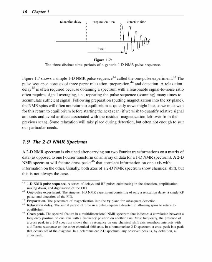
Figure 1.7 shows a simple 1-D NMR pulse sequence42 called the one-pulse experiment.43 The

pulse sequence consists of three parts: relaxation, preparation,44 and detection. A relaxation

delay45 is often required because obtaining a spectrum with a reasonable signal-to-noise ratio

often requires signal averaging, i.e., repeating the pulse sequence (scanning) many times to

accumulate sufficient signal. Following preparation (putting magnetization into the xy plane),

the NMR spins will often not return to equilibrium as quickly as we might like, so we must wait

for this return to equilibrium before starting the next scan (if we wish to quantify relative signal

amounts and avoid artifacts associated with the residual magnetization left over from the

previous scan). Some relaxation will take place during detection, but often not enough to suit

our particular needs.

1.9 The 2-D NMR Spectrum

A 2-D NMR spectrum is obtained after carrying out two Fourier transformations on a matrix of

data (as opposed to one Fourier transform on an array of data for a 1-D NMR spectrum). A 2-D

NMR spectrum will feature cross peaks46 that correlate information on one axis with

information on the other. Usually, both axes of a 2-D NMR spectrum show chemical shift, but

this is not always the case.

Figure 1.7:The three distinct time periods of a generic 1-D NMR pulse sequence.

42 1-D NMR pulse sequence. A series of delays and RF pulses culminating in the detection, amplification,mixing down, and digitization of the FID.

43 One-pulse experiment. The simplest 1-D NMR experiment consisting of only a relaxation delay, a single RFpulse, and detection of the FID.

44 Preparation. The placement of magnetization into the xy plane for subsequent detection.45 Relaxation delay. The initial period of time in a pulse sequence devoted to allowing spins to return to

equilibrium.46 Cross peak. The spectral feature in a multidimensional NMR spectrum that indicates a correlation between a

frequency position on one axis with a frequency position on another axis. Most frequently, the presence ofa cross peak in a 2-D spectrum shows that a resonance on one chemical shift axis somehow interacts witha different resonance on the other chemical shift axis. In a homonuclear 2-D spectrum, a cross peak is a peakthat occurs off of the diagonal. In a heteronuclear 2-D spectrum, any observed peak is, by definition, across peak.

16 Chapter 1

The pulse sequence used to collect a 2-D NMR data set differs only slightly (at this level of

abstraction) from the 1-D NMR pulse sequence. Figure 1.8 shows a generic 2-D NMR pulse

sequence. The 2-D pulse sequence contains four parts instead of three. The four parts of the

2-D pulse sequence are relaxation, evolution, mixing, and detection. The careful reader will

note that preparation has been split into two parts: evolution and mixing. Many 2-D

experiments are carried out with a significantly reduced relaxation delay, meaning that

equilibrium net magnetization vectors are not achieved at the start of the evolution period of the

pulse sequence.

Evolution involves imparting phase character47 to the spins in the sample. Mixing48 involves

having the phase-encoded spins pass their phase information to other spins. Evolution usually

occurs prior to mixing and is termed t1 (not to be confused with the relaxation time T1!), but in

some 2-D NMR pulse sequences the distinction between evolution and mixing is blurred, e.g.,

in the correlation spectroscopy (COSY) experiment. Evolution often starts with a pulse to put

some magnetization into the xy plane. Once in the xy plane, the magnetization will precess or

evolve (hence the name “evolution”) and, depending on the t1 evolution time,49 will precess

a certain number of degrees from its starting point. How far each set of chemically distinct

spins evolves is a function of the t1 evolution time and each spin set’s precession frequency

relative to a reference frequency. The precession frequency, therefore, depends on chemical

environment. Thus, a series of passes through the pulse sequence using different t1’s will

Figure 1.8:The four distinct time periods of a generic 2-D NMR pulse sequence.

47 Phase character. The absorptive or dispersive nature of a spectral peak. The angle by which magnetizationprecesses in the xy plane over a given time interval.

48 Mixing. The time interval in a 2-D NMR pulse sequence wherein t1-encoded phase information is passed fromspin to spin.

49 Evolution time, t1. The time period(s) in a 2-D pulse sequence during which a net magnetization is allowed toprecess in the xy plane prior to (separate mixing and) detection. In the case of the COSY experiment, theevolution and mixing times occur simultaneously. Variation of the t1 delay in a 2-D pulse sequence generatesthe t1 time domain.

Introduction 17

encode each chemically distinct set of spins with a unique array of phases in the xy plane.

During the mixing time, the phase-encoded spins are allowed to mix with each other or with

other spins. The nature of the mixing that takes place during a 2-D pulse sequence varies

widely and includes mechanisms involving through-space relaxation, through-bond

perturbations (scalar coupling), and other interactions.

During the detection period50 denoted t2 (not the relaxation time T2!), the NMR signal is

captured electronically and stored in a computer for subsequent workup. Although

detection occurs after evolution, the first Fourier transformation is applied to the time

domain data detected during the t2 detection period to generate the f2 frequency axis; that

is, the t2 time domain is converted using the Fourier transformation into the f2 frequency

domain51 before the t1 time domain is converted to the f1 frequency domain.52 This

ordering may seem counterintuitive, but recall that t1 and t2 get their names from the order

in which they occur in the pulse sequence, and not from the order in which the axes of the

data set are processed.

Following conversion of t2 to f2, we have a half-processed NMR data matrix called an

interferogram.53 The interferogram is not a particularly useful thing in and of itself, but

performing a Fourier transformation to convert the t1 time domain to the f1 frequency domain

renders a data matrix with two frequency axes (f154 and f2

55) that will (hopefully) allow the

extraction of meaningful data pertaining to our sample. Examination of the interferogram can

reveal if RF heating of the sample has occurred during the course of the data acquisition,

however, by showing that one or more resonances has shifted its position over time (this leads

to terrible artifacts in the processed 2-D spectrum).

1.10 Information Content Available Using NMR Spectroscopy

NMR spectroscopy can provide a wealth of information about the nature of solute molecules

and solute-solvent interactions. At this point, it is best to highlight the simplest and most

50 Detection period. The time period in the pulse sequence during which the FID is digitized. For a 1-D pulsesequence, this time period is denoted t1. For a 2-D pulse sequence, this time period is denoted t2.

51 f2 frequency domain. The frequency domain generated following the Fourier transformation of the t2 timedomain. The f2 frequency domain is almost exclusively used for 1H chemical shifts.

52 f1 frequency domain. The frequency domain generated following the Fourier transformation of the t1 timedomain. The f1 frequency domain most often used for 1H or 13C chemical shifts.

53 Interferogram. A 2-D data matrix that has only undergone Fourier transformation along one axis to convertthe t2 time domain to the f2 frequency domain. An interferogram will therefore show the f2 frequency domainon one axis and the t1 time domain on the other axis.

54 F1 axis, f1 axis. Syn. f1 frequency axis. The reference scale applied to the f1 frequency domain. The f1 axismay be labeled with either ppm or Hz.

55 F2 axis, f2 axis. Syn. f2 frequency axis. The reference scale applied to the f2 frequency domain. The f2 axismay be labeled with either ppm or Hz.

18 Chapter 1

basic features present in typical solution state NMR spectra, especially those of proton NMR

spectra.

• NMR provides chemical shifts (denoted d) for atoms in differing chemical environments.

For example, an aldehyde proton will show a different chemical shift than a methyl proton.

• NMR also can give the relative population of spins in each chemical environment through

peak area determination (integration).56

• NMR shows how one spin may be near (in terms of number of bonds distant) another spin

through scalar coupling or J-coupling.

• NMR also can show, through the nuclear Overhauser effect (NOE), how one atom in

a molecule may be nearby (in space) to another atom in the same or even a different

molecule.

• NMR shows, through the J-coupling of spins only a few bonds distant or through the NOE ,

how a molecule may be folded or bent.

• NMR can reveal how molecular dynamics and chemical exchange may be taking place

over a wide range of time scales.

If we acquire a reasonable grasp of the items above as a result of reading this book and

working its problems, then we will have done well. As with many disciplines (perhaps all

except particle physics), we have to accept limits to understanding, accept the notion of the

black box wherein some behavior goes in and something happens as a result that is

unfathomed (but not unfathomable), and relegate the particulars to others more well versed in

the particular field in question. Being simply aware of the realm of molecular dynamics and

knowing whom we might ask is probably a good start. In general, this quest begins with us

consulting our local NMR authority. If we are fortunate, that person will be a distinguished

faculty member, senior scientist, or the manager of the NMR facility in our institution. The

author can personally attest to the helpfulness of the Association of Managers of Magnetic

Resonance Laboratories (AMMRL), and while membership is limited, there are ways to query

the group (perhaps through someone we may know in the group) and obtain possible

suggestions and answers to delicate NMR problems. The NMR vendors monitor AMMRL

e-mail traffic and often make it a point of pride to address issues raised relating to their

own products in a timely manner.

Problems for Chapter One

Problem 1.1 What magnetic field would be required to have the RF tuned to the 1H Larmor

frequency have a wavelength of 500 nm, such that visible light would induce

transitions between allowed spin states?

56 Integration. The measurement of the area of one or more resonances in a 1-D spectrum, or the measurement ofthe volume of a cross peak in a 2-D spectrum.

Introduction 19

Problem 1.2 How many 13C spins are present in the 0.7 mL sample of 10 mM chloroform

(CHCl3)?

Problem 1.3 In an 11.74 T magnetic field, what fraction of the 13C spins will reside in the

lower energy spin state?

Problem 1.4 For an isolated methine (CH) group at a given magnetic field strength, how much

smaller is the 13C net magnetization vector compared to that of the 1H net

magnetization vector?

Problem 1.5 Neglecting line broadening effects, which of the following two samples will show

a stronger 1H NMR signal? A 15 mM sample at 20 �C or an 18 mM sample at

60 �C?

20 Chapter 1