1

C H A P T E R 1

IntroductionAfter reading this chapter, you will be able to:

• define Computer-Aided-Engineering (CAE);

• discuss different types of numerical methods;

• explain Finite Element Analysis (FEA);

• identify the importance and benefits of finite element analysis; and

• discuss ANSYS software modules/capabilities.

1.1 OVERVIEWis chapter provides an introduction to computer-aided-engineering (CAE) analysis using thefinite element method. Computer-Aided-Design (CAD) analysis examples as well as salient fea-tures of the finite element method are presented to illustrate the design analysis process. An intro-duction to ANSYS software and its capabilities and major features is provided. ANSYS softwaregraphical user interface is also briefly described.

1.2 COMPUTER-AIDEDENGINEERINGComputers are commonly used in engineering for simulating optimal prototype designs that bestmeet established performance criteria. Several mathematical and computer science-based tools arefrequently used in the construction, evaluation, and testing of design objectives and specifications.It is anticipated that in the very near future, computer modeling methods and tools will merelyrequire a formal description of the desired behavior or structure to enable automatic simulationfor product evaluation.

CAE is a technology that uses computers to analyze CAD geometry, which allows thedesigner to simulate and study how the product will function and behave so that the design can berefined and optimized. CAE software can help perform some of the steps in the design process,especially steps related to geometric modeling, analysis and synthesis. CAE tools/systems areavailable for a wide range of analyses. ese include dynamics analysis, FEA, general purpose, andothers. e dynamics analysis includes the kinematics of bodies and deals with motion and forceconcepts. Several CAE analysis packages such as ANSYS, ABAQUS, COMSOL, and otherscan calculate the resultant stresses of a design assembly with complex geometry by specifying the

2 1. INTRODUCTION

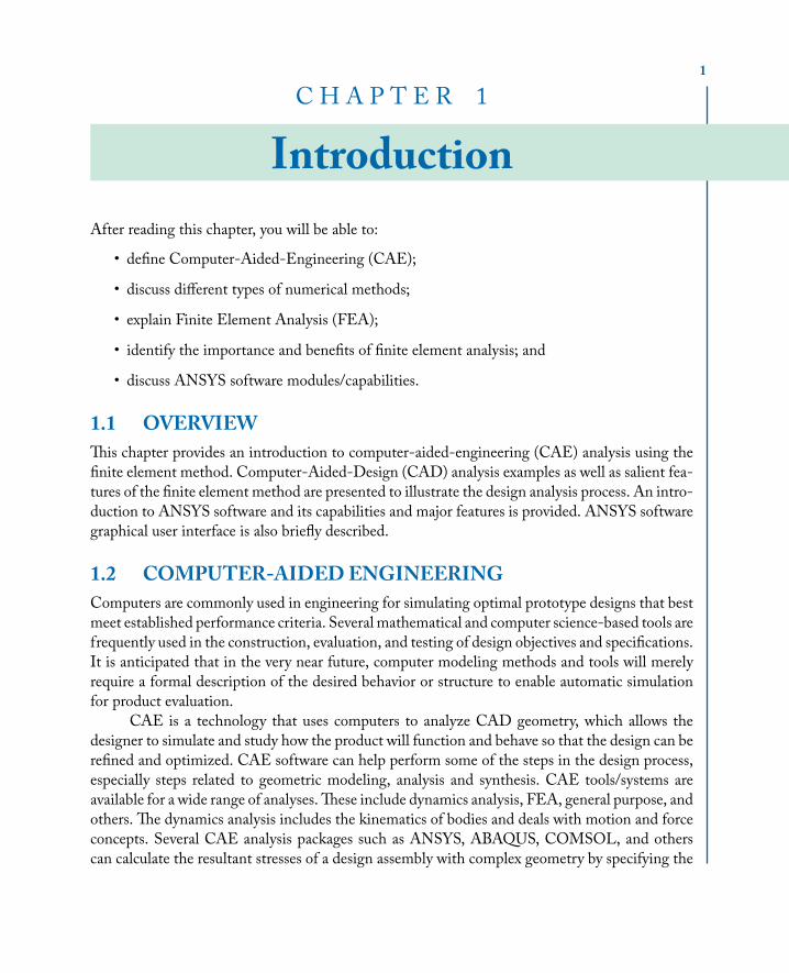
loads and using fundamental equations of statics and numerical methods. ese packages can beused for design analysis of heat transfer, fluid flow, electromagnetics, piezoelectric, and multi-physics problems. en, the structural deformation/stresses can be displayed using simulationmodels. Figure 1.1 shows the overall procedure for CAE and outlines the analysis results used toredesign the part. Design analysis techniques using various types of numerical methods are brieflydescribed in the next section.

CAD

CAE

Product

Concept

CAD

CAE

Product

ConceptConcept

CAD

CAE

Product

Figure 1.1: CAE approach to product design analysis and synthesis (source: http://www.lozik.h1.ru/).

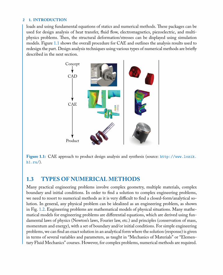
1.3 TYPESOFNUMERICALMETHODSMany practical engineering problems involve complex geometry, multiple materials, complexboundary and initial conditions. In order to find a solution to complex engineering problems,we need to resort to numerical methods as it is very difficult to find a closed-form/analytical so-lution. In general, any physical problem can be idealized as an engineering problem, as shownin Fig. 1.2. Engineering problems are mathematical models of physical situations. Many mathe-matical models for engineering problems are differential equations, which are derived using fun-damental laws of physics (Newton’s laws, Fourier law, etc.) and principles (conservation of mass,momentum and energy), with a set of boundary and/or initial conditions. For simple engineeringproblems, we can find an exact solution in an analytical formwhere the solution (response) is givenin terms of several variables and parameters, as taught in “Mechanics of Materials” or “Elemen-tary Fluid Mechanics” courses. However, for complex problems, numerical methods are required.

1.4. FINITEELEMENTANALYSIS 3

ese include the Finite Difference Method (FDM), where derivatives are replaced by differenceequations and the Finite Element Method (FEM) and the Boundary Element method (BEM)which use integral formulations to create a system of algebraic equations. In FEM, the wholedomain/geometry is discretized whereas in the BEM, the boundary of the domain/geometry isdiscretized. e finite element design analysis techniques are discussed in the next section.

Physical Problem Engineering Problem

Laws ofPhysics Governing Di!erential

Equation

Apply B.C/I.C → SOLUTION

Analytical Numerical

Behavior/Response

1. Finite Di!erence Method (FDM)

2. Finite Element Method (FEM)3. Boundary Element Method (BEM)

Figure 1.2: An overview of solutions to a physical problem.

1.4 FINITEELEMENTANALYSISFinite element analysis (FEA) is a general numerical method capable of solving a variety of en-gineering problems and the underlying theory is more than 100 years old, dating back to early1900s. Major companies including Boeing, Ford, General Electric, Intel, IBM, Apple, and oth-ers employ general purpose computer software to efficiently complete daily engineering analysistasks.

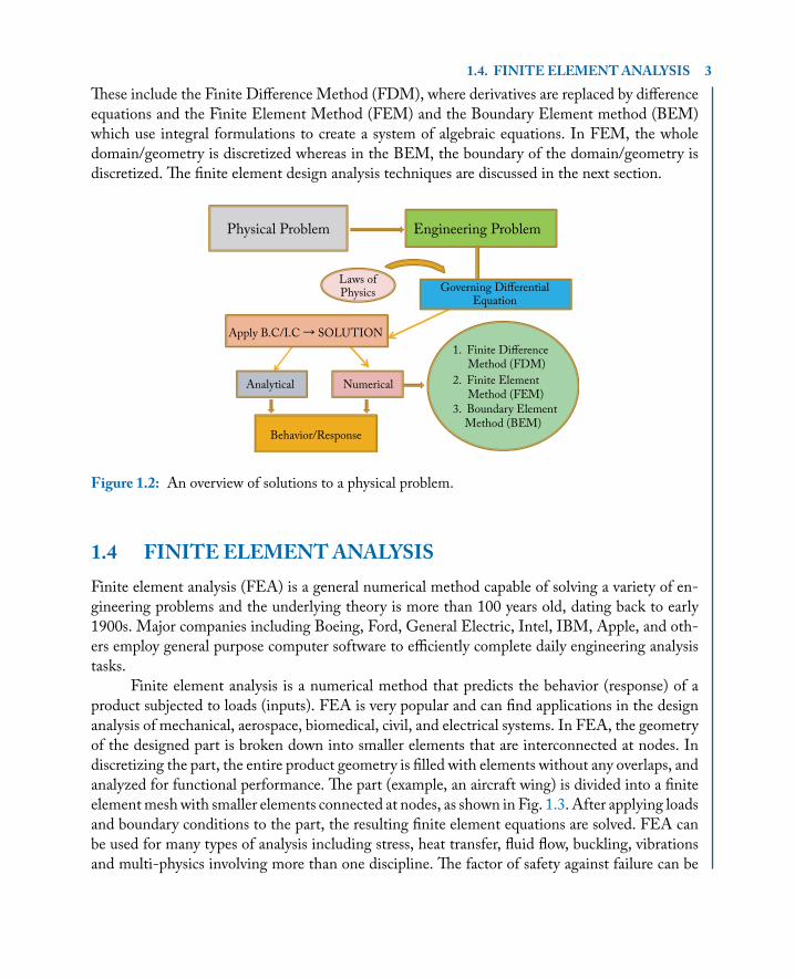
Finite element analysis is a numerical method that predicts the behavior (response) of aproduct subjected to loads (inputs). FEA is very popular and can find applications in the designanalysis of mechanical, aerospace, biomedical, civil, and electrical systems. In FEA, the geometryof the designed part is broken down into smaller elements that are interconnected at nodes. Indiscretizing the part, the entire product geometry is filled with elements without any overlaps, andanalyzed for functional performance. e part (example, an aircraft wing) is divided into a finiteelementmeshwith smaller elements connected at nodes, as shown in Fig. 1.3. After applying loadsand boundary conditions to the part, the resulting finite element equations are solved. FEA canbe used for many types of analysis including stress, heat transfer, fluid flow, buckling, vibrationsand multi-physics involving more than one discipline. e factor of safety against failure can be

4 1. INTRODUCTION

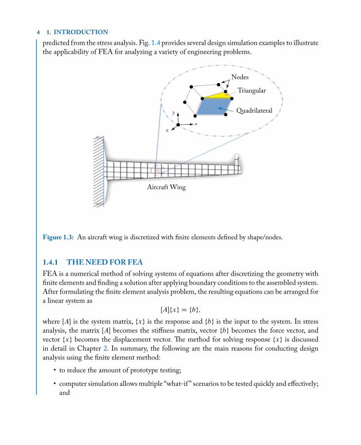
predicted from the stress analysis. Fig. 1.4 provides several design simulation examples to illustratethe applicability of FEA for analyzing a variety of engineering problems.

y

xz

Aircraft Wing

y

xz

Aircraft Wing

Nodes

Triangular

Quadrilateral

Figure 1.3: An aircraft wing is discretized with finite elements defined by shape/nodes.

1.4.1 THENEEDFORFEAFEA is a numerical method of solving systems of equations after discretizing the geometry withfinite elements and finding a solution after applying boundary conditions to the assembled system.After formulating the finite element analysis problem, the resulting equations can be arranged fora linear system as

ŒA�fxg D fbg;

where ŒA� is the system matrix, fxg is the response and fbg is the input to the system. In stressanalysis, the matrix ŒA� becomes the stiffness matrix, vector fbg becomes the force vector, andvector fxg becomes the displacement vector. e method for solving response fxg is discussedin detail in Chapter 2. In summary, the following are the main reasons for conducting designanalysis using the finite element method:

• to reduce the amount of prototype testing;

• computer simulation allowsmultiple “what-if ” scenarios to be tested quickly and effectively;and

1.4. FINITEELEMENTANALYSIS 5

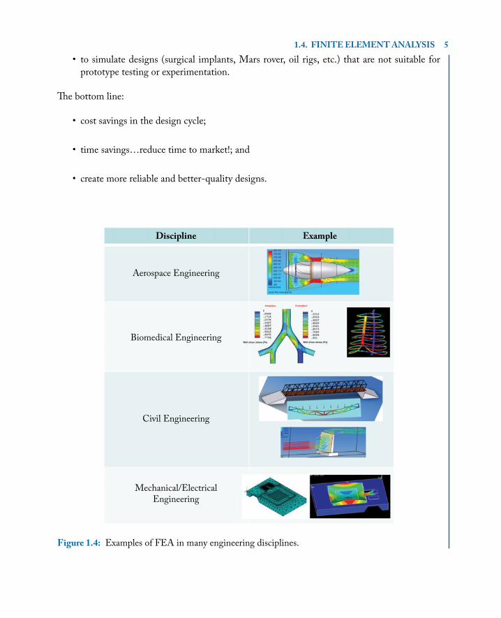
• to simulate designs (surgical implants, Mars rover, oil rigs, etc.) that are not suitable forprototype testing or experimentation.

e bottom line:

• cost savings in the design cycle;

• time savings…reduce time to market!; and

• create more reliable and better-quality designs.

Discipline Example

Aerospace Engineering

Biomedical Engineering

Civil Engineering

Mechanical/ElectricalEngineering

Figure 1.4: Examples of FEA in many engineering disciplines.

6 1. INTRODUCTION

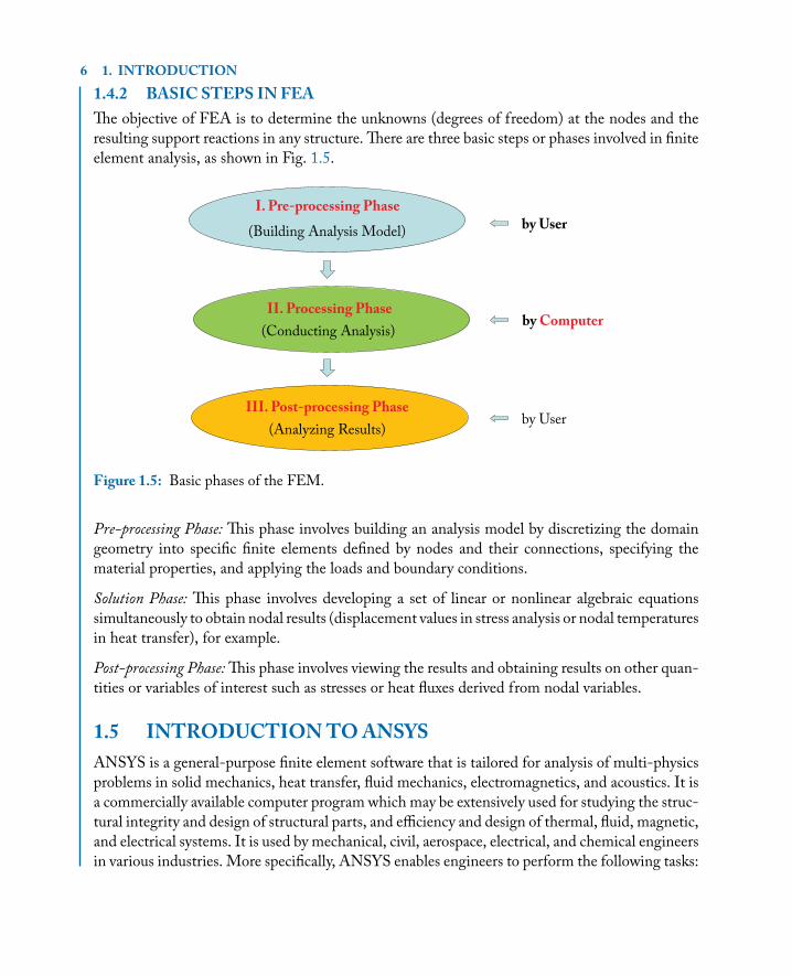
1.4.2 BASIC STEPS IN FEAe objective of FEA is to determine the unknowns (degrees of freedom) at the nodes and theresulting support reactions in any structure. ere are three basic steps or phases involved in finiteelement analysis, as shown in Fig. 1.5.

(Building Analysis Model)

(Conducting Analysis)

(Analyzing Results)

by User

by User

by Computer

I. Pre-processing Phase

III. Post-processing Phase

II. Processing Phase

Figure 1.5: Basic phases of the FEM.

Pre-processing Phase: is phase involves building an analysis model by discretizing the domaingeometry into specific finite elements defined by nodes and their connections, specifying thematerial properties, and applying the loads and boundary conditions.

Solution Phase: is phase involves developing a set of linear or nonlinear algebraic equationssimultaneously to obtain nodal results (displacement values in stress analysis or nodal temperaturesin heat transfer), for example.

Post-processing Phase:is phase involves viewing the results and obtaining results on other quan-tities or variables of interest such as stresses or heat fluxes derived from nodal variables.

1.5 INTRODUCTIONTOANSYSANSYS is a general-purpose finite element software that is tailored for analysis of multi-physicsproblems in solid mechanics, heat transfer, fluid mechanics, electromagnetics, and acoustics. It isa commercially available computer program which may be extensively used for studying the struc-tural integrity and design of structural parts, and efficiency and design of thermal, fluid, magnetic,and electrical systems. It is used by mechanical, civil, aerospace, electrical, and chemical engineersin various industries. More specifically, ANSYS enables engineers to perform the following tasks:

1.5. INTRODUCTIONTOANSYS 7

• Build computer models or transfer CAD models of structures, products, components, orsystems.

• Apply operating loads or design performance conditions.

• Study the physical responses, such as stress levels, temperature distributions, or the impactof electromagnetic fields.

• Optimize a design early in the development process to reduce production costs.

• Perform prototype testing in environments where it otherwise would be undesirable or im-possible (for example biomedical applications).

e ANSYS software has a comprehensive graphical user interface that gives users easy,interactive access to program functions, commands, documentation, and reference material.

1.5.1 ANSYSMODULESANSYS software has the following modules.

ANSYS/Multiphysics. is is a most comprehensive product which includes all other ANSYSmodules. Capabilities include structural, thermal, fluid, electromagnetic, and acoustic anal-yses. Coupling between structural, acoustic, electromagnetic, fluid, and thermal fields is alsopossible.

ANSYS/Structural. is module includes structural analysis capabilities for static and dynamicstress analysis of structures including the buckling and geometrical/material nonlinearitiesencountered in certain structures.

ANSYS/Mechanical. is module includes ANSYS/Structural with additional capabilities forlinear/nonlinear and steady/transient heat transfer and acoustics analysis capabilities. Cou-pled thermal-structural and acoustic-structural analyses can also be performed.

ANSYS/LinearPlus. is module is restricted to linear static and dynamic analysis of structures.

ANSYS/ermal. ismodule is restricted to steady/transient and linear/nonlinear heat transferanalysis of solids.

ANSYS/Emag. is module is designed for electromagnetics and electrostatics analysis of, elec-trical systems, motors, alternators, radars, etc.

ANSYS/Flotran. is Computational Fluid Dynamics Module (CFD) analyzes viscous, turbu-lent, incompressible and compressible fluid flow problems with and without heat transfer,including models for multi-species.

8 1. INTRODUCTION

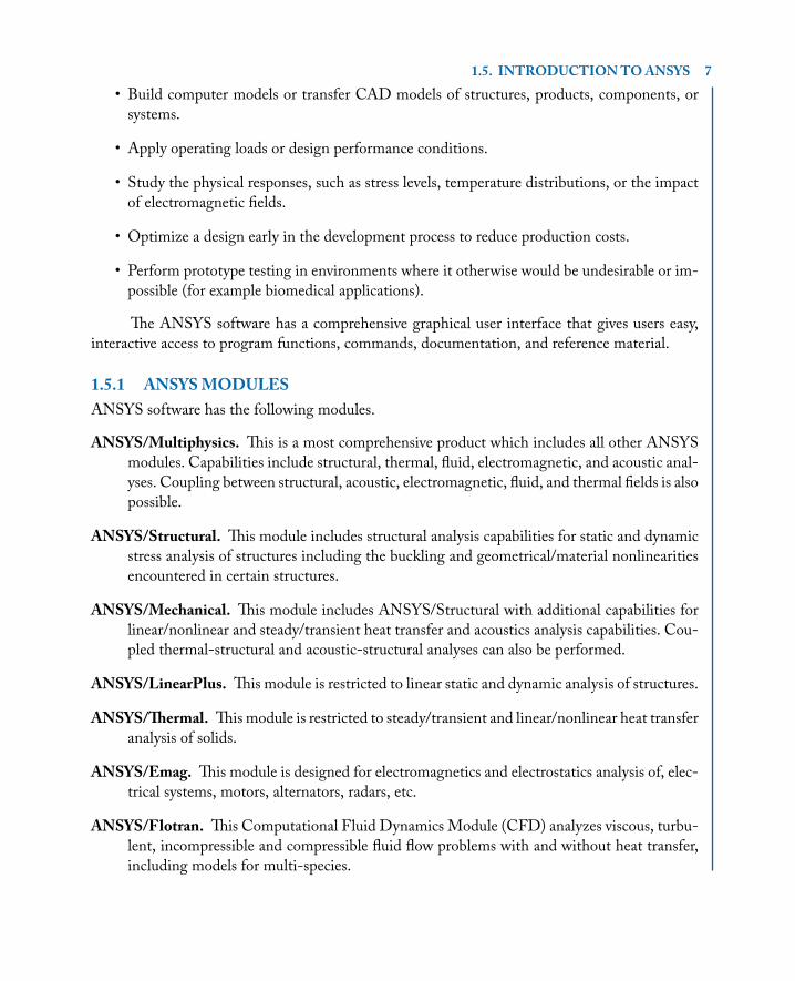
1.5.2 USINGANSYSe simplest way to enter the ANSYS program is through the ANSYS Launcher, as shown inFig. 1.6. e launcher has a menu containing push buttons that provide the choices you need torun the ANSYS program and other auxiliary programs.

Figure 1.6: e ANSYS Launcher dialog box.

When using the Launcher to enter ANSYS, follow these basic steps:

• From the Start menu select Programs ! ANSYS 14.0 ! Mechanical APDL ProductLauncher.

• e ANSYS Launcher dialog box will appear, containing interactive entry options.

Working directory. is directory is the one in which the ANSYS run will be executed. If thedirectory displayed is not the one you want to work in pick the “Browse…” button to the rightof the directory name and specify the desired directory. Note the directories you can use on en-gineering computers are on your home directory, H:, and USB flash drive E:.

Jobname. e jobname is the one that will be used as the prefix of the file name for all files gen-erated by the ANSYS run. Type the desired jobname in this field of the dialog box (the extensionfor the file names will be .DB).

GUI configuration. is command brings up a dialog box that allows you to choose the desiredmenu layout and font size. Do not change the default settings, but simply press OK on thisdialog box so that the proper settings file is created for the terminal you are using. is step isonly required the first time you enter ANSYS.

A typical analysis in ANSYS involves three distinct steps.

1.5. INTRODUCTIONTOANSYS 9

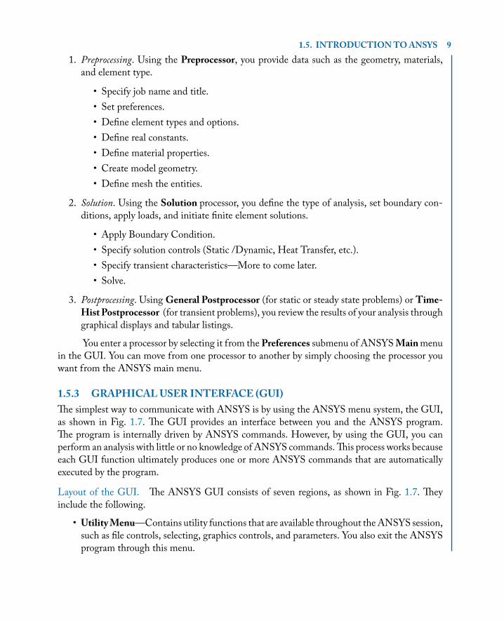
1. Preprocessing. Using the Preprocessor, you provide data such as the geometry, materials,and element type.

• Specify job name and title.• Set preferences.• Define element types and options.• Define real constants.• Define material properties.• Create model geometry.• Define mesh the entities.

2. Solution. Using the Solution processor, you define the type of analysis, set boundary con-ditions, apply loads, and initiate finite element solutions.

• Apply Boundary Condition.• Specify solution controls (Static /Dynamic, Heat Transfer, etc.).• Specify transient characteristics—More to come later.• Solve.

3. Postprocessing. Using General Postprocessor (for static or steady state problems) or Time-HistPostprocessor (for transient problems), you review the results of your analysis throughgraphical displays and tabular listings.

You enter a processor by selecting it from the Preferences submenu of ANSYSMainmenuin the GUI. You can move from one processor to another by simply choosing the processor youwant from the ANSYS main menu.

1.5.3 GRAPHICALUSER INTERFACE (GUI)e simplest way to communicate with ANSYS is by using the ANSYS menu system, the GUI,as shown in Fig. 1.7. e GUI provides an interface between you and the ANSYS program.e program is internally driven by ANSYS commands. However, by using the GUI, you canperform an analysis with little or no knowledge of ANSYS commands.is process works becauseeach GUI function ultimately produces one or more ANSYS commands that are automaticallyexecuted by the program.

Layout of the GUI. e ANSYS GUI consists of seven regions, as shown in Fig. 1.7. eyinclude the following.

• UtilityMenu—Contains utility functions that are available throughout theANSYS session,such as file controls, selecting, graphics controls, and parameters. You also exit the ANSYSprogram through this menu.

10 1. INTRODUCTION

• Command Input Area—Allows you to type in commands directly. All previously typed incommands can be viewed using the drop down arrow to the right of the command inputarea.

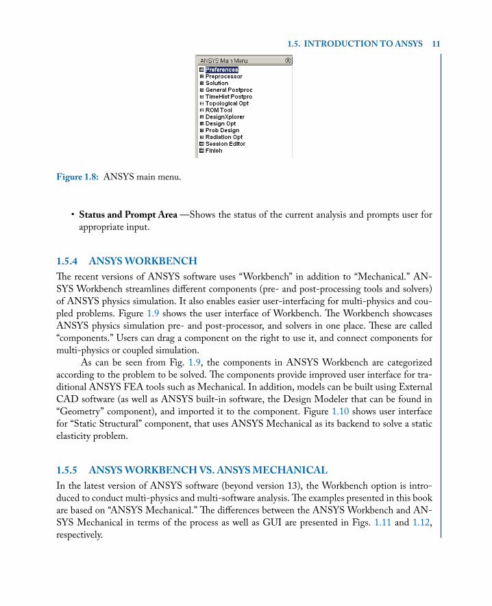
• Main Menu—Contains the primary ANSYS functions, organized by processors (prepro-cessor, solution, general postprocessor, design optimizer, etc.), as shown in Fig. 1.8.

• OutputWindow—Receives text output from the program. It is usually positioned behindthe other windows, but you can bring it to the front when necessary.

• Toolbar—Contains push buttons that execute commonly used ANSYS commands andfunctions. You may add your own push buttons by defining abbreviations.

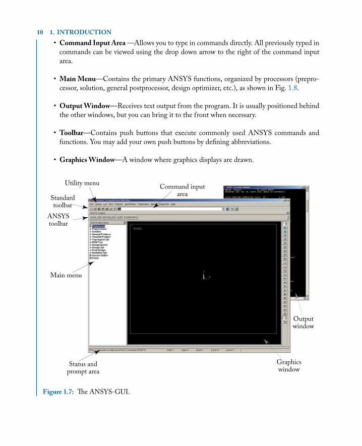
• GraphicsWindow—A window where graphics displays are drawn.

Command inputarea

Utility menu

Standardtoolbar

ANSYStoolbar

Main menu

Status andprompt area

Graphicswindow

Outputwindow

Figure 1.7: e ANSYS-GUI.

1.5. INTRODUCTIONTOANSYS 11

Figure 1.8: ANSYS main menu.

• Status and Prompt Area —Shows the status of the current analysis and prompts user forappropriate input.

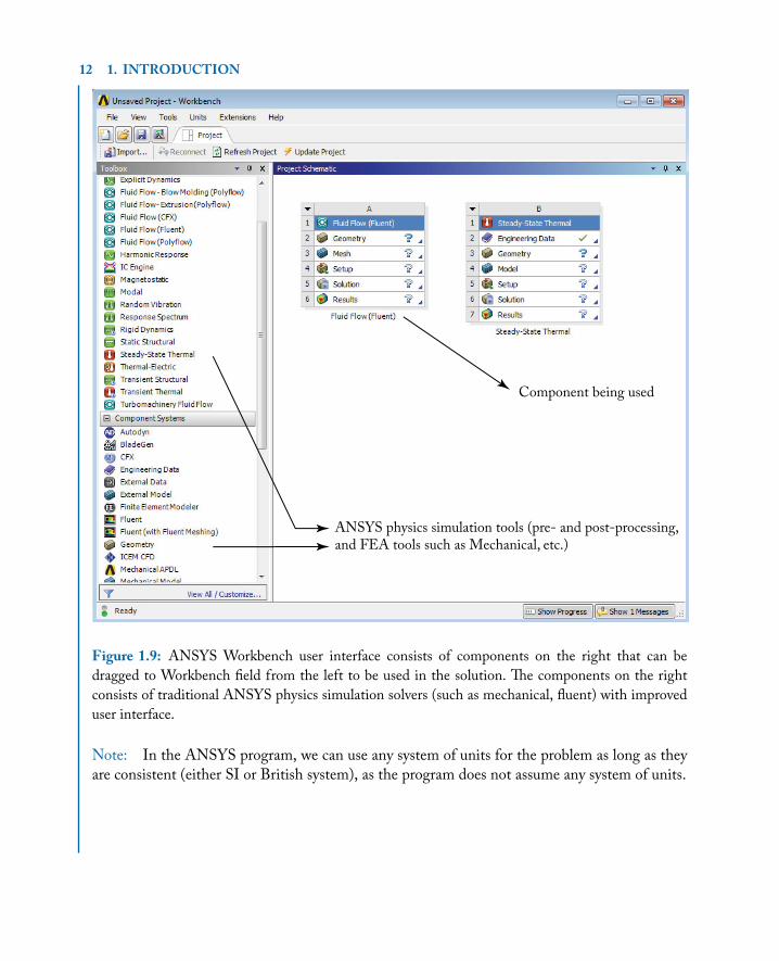
1.5.4 ANSYSWORKBENCHe recent versions of ANSYS software uses “Workbench” in addition to “Mechanical.” AN-SYS Workbench streamlines different components (pre- and post-processing tools and solvers)of ANSYS physics simulation. It also enables easier user-interfacing for multi-physics and cou-pled problems. Figure 1.9 shows the user interface of Workbench. e Workbench showcasesANSYS physics simulation pre- and post-processor, and solvers in one place. ese are called“components.” Users can drag a component on the right to use it, and connect components formulti-physics or coupled simulation.

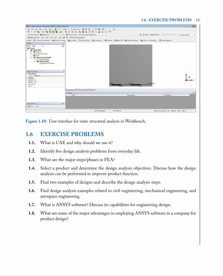
As can be seen from Fig. 1.9, the components in ANSYS Workbench are categorizedaccording to the problem to be solved. e components provide improved user interface for tra-ditional ANSYS FEA tools such as Mechanical. In addition, models can be built using ExternalCAD software (as well as ANSYS built-in software, the Design Modeler that can be found in“Geometry” component), and imported it to the component. Figure 1.10 shows user interfacefor “Static Structural” component, that uses ANSYS Mechanical as its backend to solve a staticelasticity problem.

1.5.5 ANSYSWORKBENCHVS. ANSYSMECHANICALIn the latest version of ANSYS software (beyond version 13), the Workbench option is intro-duced to conduct multi-physics and multi-software analysis. e examples presented in this bookare based on “ANSYS Mechanical.” e differences between the ANSYS Workbench and AN-SYS Mechanical in terms of the process as well as GUI are presented in Figs. 1.11 and 1.12,respectively.

12 1. INTRODUCTION

Component being used

ANSYS physics simulation tools (pre- and post-processing,and FEA tools such as Mechanical, etc.)

Figure 1.9: ANSYS Workbench user interface consists of components on the right that can bedragged to Workbench field from the left to be used in the solution. e components on the rightconsists of traditional ANSYS physics simulation solvers (such as mechanical, fluent) with improveduser interface.

Note: In the ANSYS program, we can use any system of units for the problem as long as theyare consistent (either SI or British system), as the program does not assume any system of units.

1.6. EXERCISE PROBLEMS 13

Figure 1.10: User interface for static structural analysis in Workbench.

1.6 EXERCISE PROBLEMS1.1. What is CAE and why should we use it?

1.2. Identify five design analysis problems from everyday life.

1.3. What are the major steps/phases in FEA?

1.4. Select a product and determine the design analysis objectives. Discuss how the designanalysis can be performed to improve product function.

1.5. Find two examples of designs and describe the design analysis steps.

1.6. Find design analysis examples related to civil engineering, mechanical engineering, andaerospace engineering.

1.7. What is ANSYS software? Discuss its capabilities for engineering design.

1.8. What are some of the major advantages in employing ANSYS software in a company forproduct design?

14 1. INTRODUCTION

Workbench Mechanical

Build Model Pre-ProcessingBuild Model/Mesh

Apply Material Properties

Apply BoundaryConditions

Assign Material Properties

Generate Mesh

Solver Solution

Post-Procrssing

Determine the solvercomponent(s) necessary

Apply appropriateBoundary Conditions

Generate resultsvisualization

P Design Modeler(Geometrycomponent)

P SolidWorks/AutoDesk

(a) (b)

ANYSYS CFX (for !uidand structural)

Tasks accomplished foranalysis within thecomponents:

P Transient/Steady

State Structural

P Transient/Steady

"ermal

P Fluent

P Explicit Dynamics

P Vibration

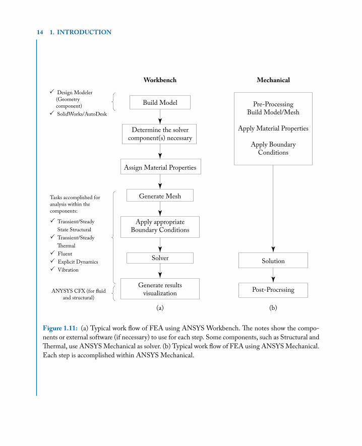
Figure 1.11: (a) Typical work flow of FEA using ANSYS Workbench. e notes show the compo-nents or external software (if necessary) to use for each step. Some components, such as Structural andermal, use ANSYS Mechanical as solver. (b) Typical work flow of FEA using ANSYS Mechanical.Each step is accomplished within ANSYS Mechanical.

1.6. EXERCISE PROBLEMS 15

Build ModelManage Material Properties

Mesh, Boundary Condition,Solution, and Post-Processing

Pre-ProcessingBuild Model/MeshMaterial Properties

Post-Processing

Solution

(a) (b)

Workbench Mechanical

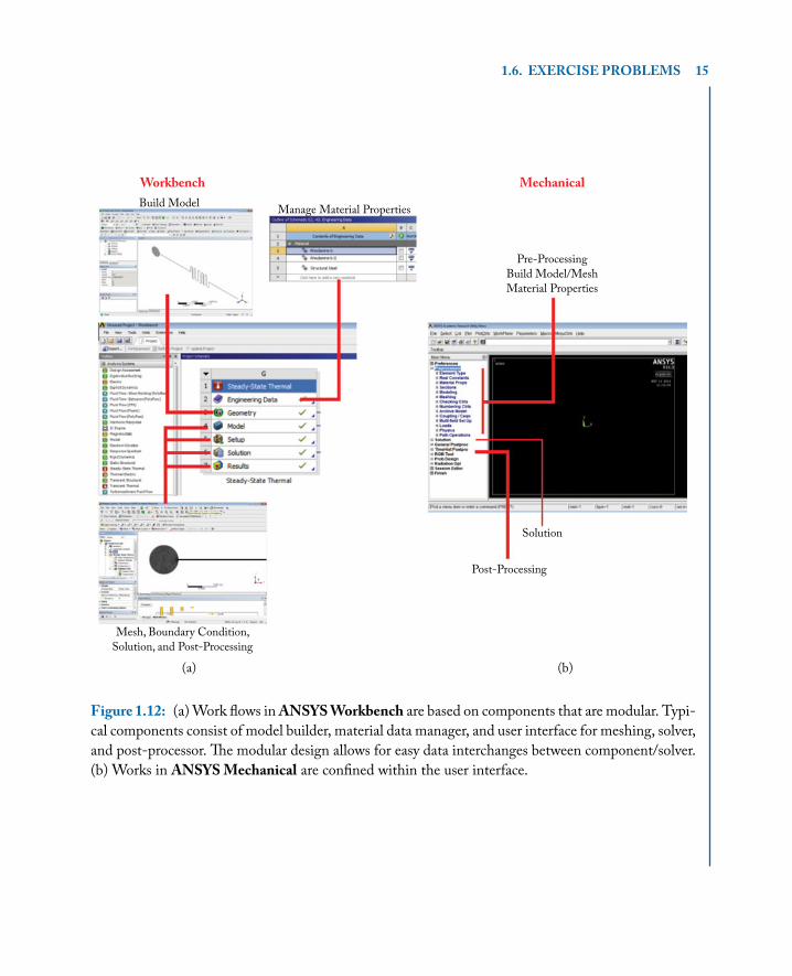
Figure 1.12: (a) Work flows inANSYSWorkbench are based on components that are modular. Typi-cal components consist of model builder, material data manager, and user interface for meshing, solver,and post-processor. e modular design allows for easy data interchanges between component/solver.(b) Works in ANSYSMechanical are confined within the user interface.

17

C H A P T E R 2

Mathematical PreliminariesAfter reading this chapter, you will be able to:

• explain matrices and their basic operations;

• find a solution to a matrix system of equations;

• find eigenvalues and eigenvectors of a matrix/system;

• evaluate an integral numerically; and

• use MATLAB to solve matrix algebra problems.

2.1 OVERVIEW

is chapter introduces matrix algebra, and discusses example procedures for solving matrix sys-tems of equations and eigenvalue problems. An introduction to numerical integration is also pre-sented as it is commonly used in finite element analysis. MATLAB instructions for carrying outmatrix operations are also presented.

2.2 MATRIXALGEBRA

FEA uses matrix algebra and vector calculus extensively, therefore an introduction to matrix alge-bra is presented in this chapter. Also, a matrix is a convenient way to represent engineering data.Here, we review a set of matrix operations and functions that apply to finite element analysis.

Row Vector: e row vector is a collection of elements (scalars) arranged in a row that has manycolumns .n/. See for example, row vector fAg as shown below:

fAg D elements that are arranged .1xn/ as;fAg1xn D fa1; a2; : : : : : : ::ang :

18 2. MATHEMATICAL PRELIMINARIES

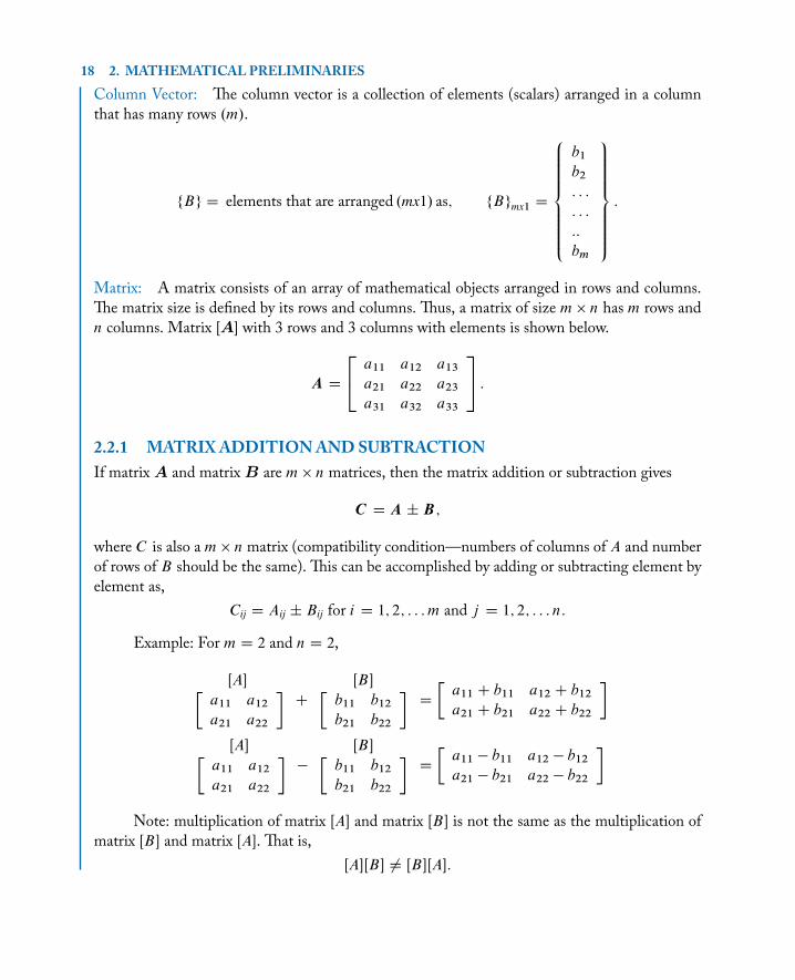
Column Vector: e column vector is a collection of elements (scalars) arranged in a columnthat has many rows .m/.

fBg D elements that are arranged .mx1/ as; fBgmx1 D

8̂̂̂̂ˆ̂̂<̂ˆ̂̂̂̂̂:

b1

b2

: : :

: : :

::

bm

9>>>>>>>=>>>>>>>;:

Matrix: A matrix consists of an array of mathematical objects arranged in rows and columns.e matrix size is defined by its rows and columns. us, a matrix of size m � n has m rows andn columns. Matrix ŒA� with 3 rows and 3 columns with elements is shown below.

A D

24 a11 a12 a13

a21 a22 a23

a31 a32 a33

35 :

2.2.1 MATRIXADDITIONANDSUBTRACTIONIf matrix A and matrix B are m � n matrices, then the matrix addition or subtraction gives

C D A ˙ B;

where C is also a m � n matrix (compatibility condition—numbers of columns of A and numberof rows of B should be the same). is can be accomplished by adding or subtracting element byelement as,

Cij D Aij ˙ Bij for i D 1; 2; : : : m and j D 1; 2; : : : n:

Example: For m D 2 and n D 2,

ŒA��a11 a12

a21 a22

�C

ŒB��b11 b12

b21 b22

�D

�a11 C b11 a12 C b12

a21 C b21 a22 C b22

�ŒA��

a11 a12

a21 a22

��

ŒB��b11 b12

b21 b22

�D

�a11 � b11 a12 � b12

a21 � b21 a22 � b22

�Note: multiplication of matrix ŒA� and matrix ŒB� is not the same as the multiplication of

matrix ŒB� and matrix ŒA�. at is,ŒA�ŒB� ¤ ŒB�ŒA�:

2.2. MATRIXALGEBRA 19

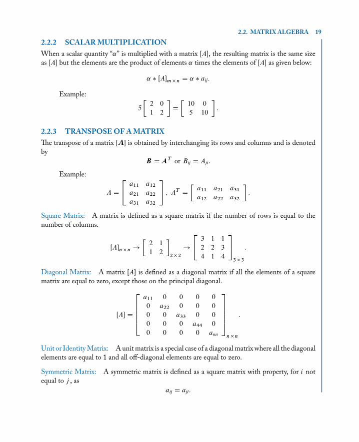
2.2.2 SCALARMULTIPLICATIONWhen a scalar quantity “˛” is multiplied with a matrix ŒA�, the resulting matrix is the same sizeas ŒA� but the elements are the product of elements ˛ times the elements of ŒA� as given below:

˛ � ŒA�m � n D ˛ � aij:

Example:

5

�2 0

1 2

�D

�10 0

5 10

�:

2.2.3 TRANSPOSEOFAMATRIXe transpose of a matrix ŒA� is obtained by interchanging its rows and columns and is denotedby

B D AT or Bij D Aji:

Example:

A D

24 a11 a12

a21 a22

a31 a32

35 ; ATD

�a11 a21 a31

a12 a22 a32

�:

Square Matrix: A matrix is defined as a square matrix if the number of rows is equal to thenumber of columns.

ŒA�n � n !

�2 1

1 2

�2 � 2

!

24 3 1 1

2 2 3

4 1 4

353 � 3

:

Diagonal Matrix: A matrix ŒA� is defined as a diagonal matrix if all the elements of a squarematrix are equal to zero, except those on the principal diagonal.

ŒA� D

266664a11 0 0 0 0

0 a22 0 0 0

0 0 a33 0 0

0 0 0 a44 0

0 0 0 0 ann

377775n � n

:

Unit or IdentityMatrix: A unitmatrix is a special case of a diagonalmatrix where all the diagonalelements are equal to 1 and all off-diagonal elements are equal to zero.

Symmetric Matrix: A symmetric matrix is defined as a square matrix with property, for i notequal to j , as

aij D aji:

20 2. MATHEMATICAL PRELIMINARIES

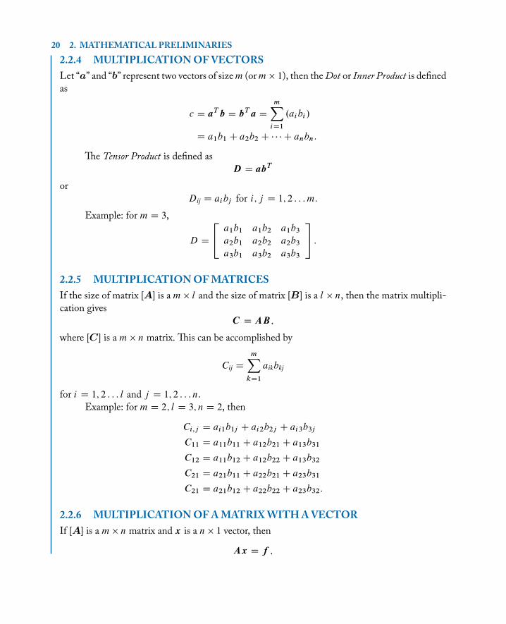
2.2.4 MULTIPLICATIONOFVECTORSLet “a” and “b” represent two vectors of size m (or m � 1), then theDot or Inner Product is definedas

c D aT b D bT a D

mXiD1

.aibi /

D a1b1 C a2b2 C � � � C anbn:

e Tensor Product is defined asD D abT

orDij D aibj for i; j D 1; 2 : : : m:

Example: for m D 3,

D D

24 a1b1 a1b2 a1b3

a2b1 a2b2 a2b3

a3b1 a3b2 a3b3

35 :

2.2.5 MULTIPLICATIONOFMATRICESIf the size of matrix ŒA� is a m � l and the size of matrix ŒB� is a l � n, then the matrix multipli-cation gives

C D AB;

where ŒC� is a m � n matrix. is can be accomplished by

Cij D

mXkD1

aikbkj

for i D 1; 2 : : : l and j D 1; 2 : : : n.Example: for m D 2; l D 3; n D 2, then

Ci;j D ai1b1j C ai2b2j C ai3b3j

C11 D a11b11 C a12b21 C a13b31

C12 D a11b12 C a12b22 C a13b32

C21 D a21b11 C a22b21 C a23b31

C21 D a21b12 C a22b22 C a23b32:

2.2.6 MULTIPLICATIONOFAMATRIXWITHAVECTORIf ŒA� is a m � n matrix and x is a n � 1 vector, then

Ax D f ;