chapter 1 introduction to matlab - computer sciencegilbert/cs290ispr2003/molermatlabintro.pdfchapter...
TRANSCRIPT
Chapter 1
Introduction to MATLAB
This book is an introduction to two subjects, numerical computing and MatlabThis first chapter introduces Matlab by presenting several sample programs thatinvestigate elementary, but hopefully interesting, mathematical problems. We hopethat you can see how Matlab works by studying these sample programs.
You should have a copy of Matlab close at hand so you can run the sampleprograms as you read about them. All of the programs used in this book have beencollected in a directory (or folder) named
NCM
(The directory name is an acronym for the book title). You can either start Matlabin this directory, or add the directory to the Matlab path.
1.1 The Golden RatioWhat is the world’s most interesting number? Perhaps you like 17, or π, or e?Many people would vote for φ, the golden ratio, computed here by our first Matlabstatement
phi = (1 + sqrt(5))/2
This produces
phi =1.6180
Let’s see more digits.
format longphi
phi =1.61803398874989
1

2 Chapter 1. Introduction to MATLAB
This didn’t recompute φ, it just displayed 15 significant digits instead of five.The golden ratio shows up in many places in mathematics; we’ll see several in
this book. It gets its name from the golden rectangle, the rectangle with the perfectaspect ratio. It has the property that removing a square leaves a smaller rectanglewith the same shape. Here it is.
φ
φ − 1
1
1
Equating the aspect ratios of the rectangles gives a defining equation for φ.
1φ
=φ− 1
1
This equation says that you can compute the reciprocal of φ by simply subtractingone. How many numbers have that property?
Multiplying the aspect ratio equation by φ produces a polynomial equation
φ2 − φ− 1 = 0
The roots of this equation are given by the quadratic formula.
φ =1±√5
2
The positive root is the golden ratio. The negative root, which is actually equal to1 − φ, has no meaning in the golden rectangle, but it will show up later in othercontexts.
If you have forgotten the quadratic formula, you can ask Matlab to findthe roots of the polynomial. Matlab represents a polynomial by the vector of itscoefficients, in descending order. So the vector
p = [1 -1 -1]
represents the polynomial
p(x) = x2 − x− 1
The roots are computed by the roots function.
r = roots(p)

1.1. The Golden Ratio 3
produces
r =-0.618033988749891.61803398874989
These two numbers are the only numbers whose reciprocal can be computed bysubtracting one.
You can use the Symbolic Toolbox, which connects Matlab to Maple, tosolve the aspect ratio equation without converting it to a polynomial. The equationis represented by a character string. The solve function finds two solutions.
r = solve(’1/x = x-1’)
produces
r =[ 1/2*5^(1/2)+1/2][ 1/2-1/2*5^(1/2)]
The pretty function displays the results in a way that resembles typeset mathe-matics.
pretty(r)
produces
[ 1/2 ][1/2 5 + 1/2][ ][ 1/2][1/2 - 1/2 5 ]
The variable r is a vector with two components, the symbolic forms of the twosolutions. You can pick off the first component with
phi = r(1)
which produces
phi =1/2*5^(1/2)+1/2
This expression can be converted to a numerical value in a couple of different ways.It can be evaluated to any number of digits using variable-precision arithmetic withthe vpa function.
vpa(phi,50)
produces 50 digits
1.6180339887498948482045868343656381177203091798058

4 Chapter 1. Introduction to MATLAB
It can also be converted to double-precision floating-point, which is the principalway that Matlab represents numbers, with the double function.
phi = double(phi)
produces
phi =1.61803398874989
The aspect ratio equation is simple enough to have closed form symbolic so-lutions. More complicated equations have to be solved approximately. The inlinefunction is a quick way to convert character strings to objects that can be argumentsto the Matlab functions that operate on other functions.
f = inline(’1/x - (x-1)’);
defines f(x) = 1/x− (x− 1) and produces
f =Inline function:f(x) = 1/x - (x-1)
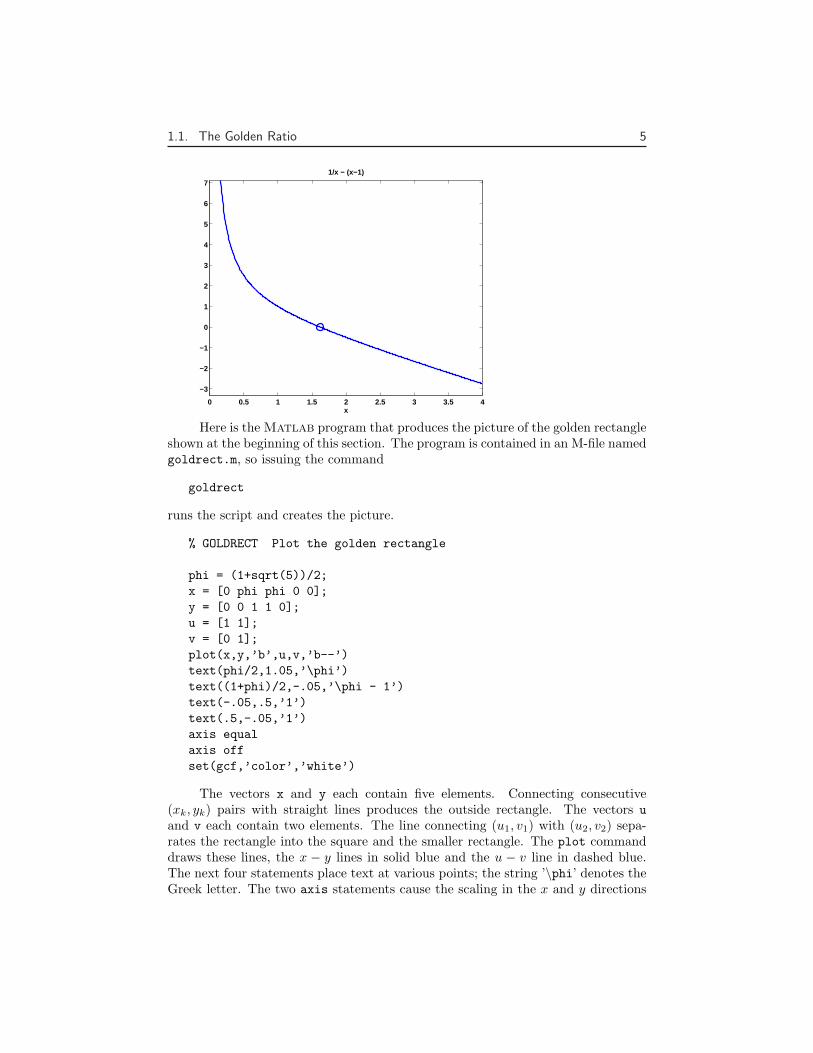
A graph of f(x) over the interval 0 ≤ x ≤ 4 is obtained with
ezplot(f,0,4)
The name ezplot stands for easy plot, although some of the English-speaking worldwould pronounce it as “e-zed plot”. Even though f(x) becomes infinite as x → 0,ezplot automatically picks a reasonable vertical scale.
The statement
phi = fzero(f,1)
looks for a zero of f(x) near x = 1. It produces an approximation to φ that isaccurate to almost full precision. The result can be inserted in the ezplot graphwith
hold onplot(phi,0,’o’)
1.1. The Golden Ratio 5
0 0.5 1 1.5 2 2.5 3 3.5 4
−3
−2
−1
0
1
2
3
4
5
6
7
x
1/x − (x−1)
Here is the Matlab program that produces the picture of the golden rectangleshown at the beginning of this section. The program is contained in an M-file namedgoldrect.m, so issuing the command
goldrect
runs the script and creates the picture.
% GOLDRECT Plot the golden rectangle
phi = (1+sqrt(5))/2;x = [0 phi phi 0 0];y = [0 0 1 1 0];u = [1 1];v = [0 1];plot(x,y,’b’,u,v,’b--’)text(phi/2,1.05,’\phi’)text((1+phi)/2,-.05,’\phi - 1’)text(-.05,.5,’1’)text(.5,-.05,’1’)axis equalaxis offset(gcf,’color’,’white’)
The vectors x and y each contain five elements. Connecting consecutive(xk, yk) pairs with straight lines produces the outside rectangle. The vectors uand v each contain two elements. The line connecting (u1, v1) with (u2, v2) sepa-rates the rectangle into the square and the smaller rectangle. The plot commanddraws these lines, the x − y lines in solid blue and the u − v line in dashed blue.The next four statements place text at various points; the string ’\phi’ denotes theGreek letter. The two axis statements cause the scaling in the x and y directions

6 Chapter 1. Introduction to MATLAB
to be equal and then turn off the display of the axes. The last statement sets thebackground color of gcf, which stands for get current figure, to white.
A continued fraction is an infinite expression of the form
a0 +1
a1 + 1a2+
1a3+...
If all the ak’s are equal to one, the continued fraction is another representation ofthe golden ratio.
φ = 1 +1
1 + 11+ 1
1+...
Here is a Matlab function that generates and evaluates truncated continued frac-tion approximations to φ. The code is stored in an M-file named goldfract.m.
function goldfract(n)% GOLDFRACT Golden ratio truncated continued fraction.% GOLDFRACT(n) displays n terms.
g = ’1’;for k = 1:n
g = [’1+1/(’ g ’)’];endg
g = 1;f = 1;for k = 1:n
s = g;g = g + f;f = s;
endg = sprintf(’%d/%d’,g,f)
format longg = eval(g)
format shorterr = (1+sqrt(5))/2 - g
The statement
goldfract(6)
produces
g =1+1/(1+1/(1+1/(1+1/(1+1/(1+1/(1))))))

1.1. The Golden Ratio 7
g =21/13
g =1.61538461538462
err =0.0026
The three g’s are all different representations of the same approximation to φ.The first g is the continued fraction truncated to six terms. There are six
right parentheses. This g is a string generated by starting with a single ’1’ (that’sgoldfract(0)) and repeatedly inserting the string ’1+1/(’ in front and the string ’)’in back. No matter how long this string becomes, it is a valid Matlab expression.
The second g is an “ordinary” fraction with a single integer numerator anddenominator obtained by collapsing the first g. The basis for the reformulation is
1 +1gf
=g + f
g
So the iteration starts with11
and repeatedly replaces the fractiong
f
by
g + f
g
The statement
g = sprintf(’%d/%d’,g,f)
prints the final fraction by formatting g and f as decimal integers and placing a ’/’between them.
The third g is the same number as the first two g’s, but is represented asa conventional decimal expansion, obtained by having the Matlab eval functionactually do the division expressed in the second g.
The final quantity err is the difference between g and φ. With only six terms,the approximation is accurate to less than three digits. How many terms does ittake to get 10 digits of accuracy?
As the number of terms n increases, the truncated continued fraction gener-ated by goldfract(n) theoretically approaches φ. But limitations on the size ofthe integers in the numerator and denominator, as well as roundoff error in theactual floating-point division, eventually intervene. One of the exercises asks youto investigate the limiting accuracy of goldfract(n).

8 Chapter 1. Introduction to MATLAB
1.2 Fibonacci NumbersLeonardo Pisano Fibonacci was born around 1170 and died around 1250 in Pisa inwhat is now Italy. He traveled extensively in Europe and Northern Africa. He wroteseveral mathematical texts that, among other things, introduced Europe to theHindu-Arabic notation for numbers. Even though his books had to be transcribedby hand, they were still widely circulated. In his best known book, Liber Abaci,published in 1202, he posed the following problem.
A man put a pair of rabbits in a place surrounded on all sides by a wall.How many pairs of rabbits can be produced from that pair in a year if itis supposed that every month each pair begets a new pair which from thesecond month on becomes productive?
Today the solution to this problem is known as the Fibonacci sequence, orFibonacci numbers. There is a small mathematical industry based on Fibonaccinumbers. A search of the Internet for “Fibonacci” will find dozens of Web sites andhundreds of pages of material. There is even a Fibonacci Association that publishesa scholarly journal, the Fibonacci Quarterly.
If Fibonacci had not specified a month for the newborn pair to mature, hewould not have a sequence named after him. The number of pairs would simplydouble each month. After n months there would be 2n pairs of rabbits. That’s alot of rabbits, but not distinctive mathematics.
Let fn denote the number of pairs of rabbits after n months. The key fact isthat the number of rabbits at the end of a month is the number at the beginningof the month plus the number of births produced by the mature pairs.
fn = fn−1 + fn−2
The initial conditions are that in the first month there is one pair of rabbits and inthe second there are two pairs.
f1 = 1, f2 = 2
Here is a Matlab function, stored in the M-file fibonacci.m, that producesa vector containing the first n Fibonacci numbers.
function f = fibonacci(n)% FIBONACCI Fibonacci sequence% f = FIBONACCI(n) generates the first n Fibonacci numbers.f = zeros(n,1);f(1) = 1;f(2) = 2;for k = 3:n
f(k) = f(k-1) + f(k-2);end
With these initial conditions, the answer to Fibonacci’s original question about thesize of the rabbit population after one year is given by

1.2. Fibonacci Numbers 9
fibonacci(12)
This produces
12358
1321345589
144233
The answer is 233 pairs of rabbits. (It would be 4096 pairs if the number doubledevery month for 12 months.)
Let’s look carefully at fibonacci.m. It’s a good example of how to create aMatlab function. The first line is
function f = fibonacci(n)
The first word on the first line says this is a function M-file, not a script. Theremainder of the first line says this particular function produces one output result,f, and takes one input argument, n. The name of the function specified on the firstline is not actually used because Matlab looks for the name of the M-file, but itis common practice to have the two match.
The next two lines are comments that provide the text displayed when youask for help.
help fibonacci
produces
FIBONACCI Fibonacci sequencef = FIBONACCI(n) generates the first n Fibonacci numbers.
Here the name of the function is in uppercase because historically Matlab was caseinsensitive and ran on terminals with only a single font. The use of capital lettersmay be confusing to some first-time Matlab users, but the convention persists. Itis important to repeat the input and output arguments in these comments becausethe first line is not displayed when you ask for help on the function.
The next line
f = zeros(n,1);
creates an n-by-1 matrix containing all zeros and assigns it to f. In Matlab, amatrix with only one column is a column vector and a matrix with only one row isa row vector.
The next two lines
10 Chapter 1. Introduction to MATLAB
f(1) = 1;f(2) = 2;
provide the initial conditions.The last three lines are the for statement that does all the work.
for k = 3:nf(k) = f(k-1) + f(k-2);
end
We like to use three spaces to indent the body of for and if statements, but otherpeople prefer two, or four, spaces, or a tab. You can also put the entire constructionon one line if you provide a comma after the first clause.
This particular function looks a lot like functions in other programming lan-guages. It produces a vector, but it does not use any of the Matlab vector ormatrix operations. We will see some of these operations soon.
Here is another Fibonacci function, fibnum.m. Its output is simply the nthFibonacci number.
function f = fibnum(n)% FIBNUM Fibonacci number.% FIBNUM(n) generates the nth Fibonacci number.if n <= 1
f = 1;else
f = fibnum(n-1) + fibnum(n-2);end
The statement
fibnum(12)
produces
ans =233
The fibnum function is recursive. In fact, the term recursive is used in both amathematical and a computer science sense. The relationship fn = fn−1 + fn−2 isknown as a recursion relation and a function that calls itself is a recursive function.
A recursive program is elegant, but expensive. You can measure executiontime with tic and toc. Try
tic, fibnum(24), toc
Do not try
tic, fibnum(50), toc
Now compare the results produced by goldfract(6) and fibonacci(7). Thefirst contains the fraction 21/13 while the second ends with 13 and 21. This is notjust a coincidence. The continued fraction is collapsed by repeating the statement

1.2. Fibonacci Numbers 11
g = g + f;
while the Fibonacci numbers are generated by
f(k) = f(k-1) + f(k-2);
In fact, if we let φn denote the golden ratio continued fraction truncated at n terms,then
fn+1
fn= φn
In the infinite limit, the ratio of successive Fibonacci numbers approaches the goldenratio.
limn→∞
fn+1
fn= φ
To see this, compute 40 Fibonacci numbers:
n = 40;f = fibonacci(n);
Then compute their ratios:
f(2:n)./f(1:n-1)
This takes the vector containing f(2) through f(n) and divides it, element byelement, by the vector containing f(1) through f(n-1). The output begins with
2.000000000000001.500000000000001.666666666666671.600000000000001.625000000000001.615384615384621.619047619047621.617647058823531.61818181818182
and ends with
1.618033988749901.618033988749891.618033988749901.618033988749891.61803398874989
Do you see why we chose n = 40? Use the up arrow key on your keyboard to bringback the previous expression. Change it to
f(2:n)./f(1:n-1) - phi
12 Chapter 1. Introduction to MATLAB
and then press the Enter key. What is the value of the last element?The population of Fibonacci’s rabbit pen doesn’t double every month; it is
multiplied by the golden ratio every month.It is possible to find a closed form solution to the Fibonacci number recurrence
relation. The key is to look for solutions of the form
fn = cρn
for some constants c and ρ. The recurrence relation
fn = fn−1 + fn−2
becomes
ρ2 = ρ + 1
We’ve seen this equation before. There are two possible values of ρ, namely φ and1− φ. The general solution to the recurrence is
fn = c1φn + c2(1− φ)n
The constants c1 and c2 are determined by initial conditions, which are nowconveniently written
f0 = c1 + c2 = 1f1 = c1φ + c2(1− φ) = 1
An exercise will ask you to use the Matlab backslash operator to solve this 2-by-2system of simultaneous linear equations, but it is actually easier to solve the systemby hand.
c1 =φ
2φ− 1
c2 = − (1− φ)2φ− 1
Inserting these in the general solution gives
fn =1
2φ− 1(φn+1 − (1− φ)n+1)
This is an amazing equation. The right-hand side involves powers and quo-tients of irrational numbers, but the result is a sequence of integers. You can checkthis with Matlab, displaying the results in scientific notation.
format long en = (1:40)’;f = (phi.^(n+1) - (1-phi).^(n+1))/(2*phi-1)
The .^ operator is an element-by-element power operator. It is not necessary touse ./ for the final division because (2*phi-1) is a scalar quantity. The computedresult starts with

1.3. Fractal Fern 13
f =1.000000000000000e+0002.000000000000000e+0003.000000000000000e+0005.000000000000001e+0008.000000000000002e+0001.300000000000000e+0012.100000000000000e+0013.400000000000001e+001
and ends with
5.702887000000007e+0069.227465000000011e+0061.493035200000002e+0072.415781700000003e+0073.908816900000005e+0076.324598600000007e+0071.023341550000001e+0081.655801410000002e+008
Roundoff error prevents the results from being exact integers, but
f = round(f)
finishes the job.
1.3 Fractal FernThe M-file fern.m produces the “Fractal Fern” described by Michael Barnsley inhis book Fractals Everywhere, published by Academic Press in 1993. It generatesand plots a potentially infinite sequence of random, but carefully choreographed,points in the plane. The command
fern
runs forever, producing an increasingly dense picture.An accurate plot of the fractal fern contains at least a few hundred thousand
points and it is impractical to reproduce high resolution output in this book. Hereis a low resolution plot with 5000 points.

14 Chapter 1. Introduction to MATLAB
We have included a compressed version of a 1024-by-768 pixel plot containing250,000 points in the NCM collection. Find the file
fern.bmp.gz
Use WinZip or gunzip to uncompress the file. This produces a 2.25 megabytebitmap file, fern.bmp, that you can view with a browser or a paint program. If youhave access to the MATLAB Image Processing Toolbox, you can view the file with
imshow(imread(’fern.bmp’))
If you like the image, you might even choose to make it your desktop background“wallpaper”. However, you should really run fern on your own computer to see thedynamics of the emerging fern in high resolution.
The fern is generated by repeated transformations of a point in the plane. Letx be a vector with two components, x1 and x2, representing the point. There arefour different transformations, all of them of the form.
x → Ax + b
with different matrices A and vectors b. These are known as affine transformations.The most frequently used transformation has
A =(
.85 .04−.04 .85
), b =
(0
1.6
)
This transformation shortens and rotates x a little bit, then adds 1.6 to its secondcomponent. Repeated application of this transformation moves the point up and tothe right, heading towards the upper tip of the fern. Every once in a while, one ofthe other three transformations is picked at random. These transformations move
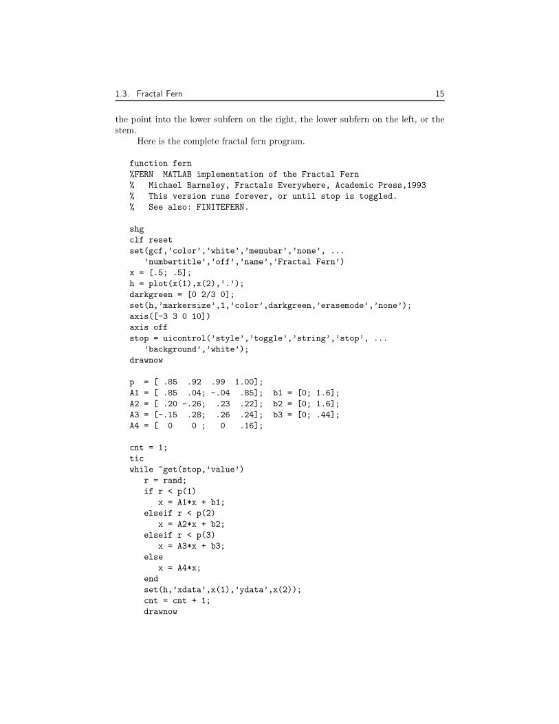
1.3. Fractal Fern 15
the point into the lower subfern on the right, the lower subfern on the left, or thestem.
Here is the complete fractal fern program.
function fern%FERN MATLAB implementation of the Fractal Fern% Michael Barnsley, Fractals Everywhere, Academic Press,1993% This version runs forever, or until stop is toggled.% See also: FINITEFERN.
shgclf resetset(gcf,’color’,’white’,’menubar’,’none’, ...
’numbertitle’,’off’,’name’,’Fractal Fern’)x = [.5; .5];h = plot(x(1),x(2),’.’);darkgreen = [0 2/3 0];set(h,’markersize’,1,’color’,darkgreen,’erasemode’,’none’);axis([-3 3 0 10])axis offstop = uicontrol(’style’,’toggle’,’string’,’stop’, ...
’background’,’white’);drawnow
p = [ .85 .92 .99 1.00];A1 = [ .85 .04; -.04 .85]; b1 = [0; 1.6];A2 = [ .20 -.26; .23 .22]; b2 = [0; 1.6];A3 = [-.15 .28; .26 .24]; b3 = [0; .44];A4 = [ 0 0 ; 0 .16];
cnt = 1;ticwhile ~get(stop,’value’)
r = rand;if r < p(1)
x = A1*x + b1;elseif r < p(2)
x = A2*x + b2;elseif r < p(3)
x = A3*x + b3;else
x = A4*x;endset(h,’xdata’,x(1),’ydata’,x(2));cnt = cnt + 1;drawnow
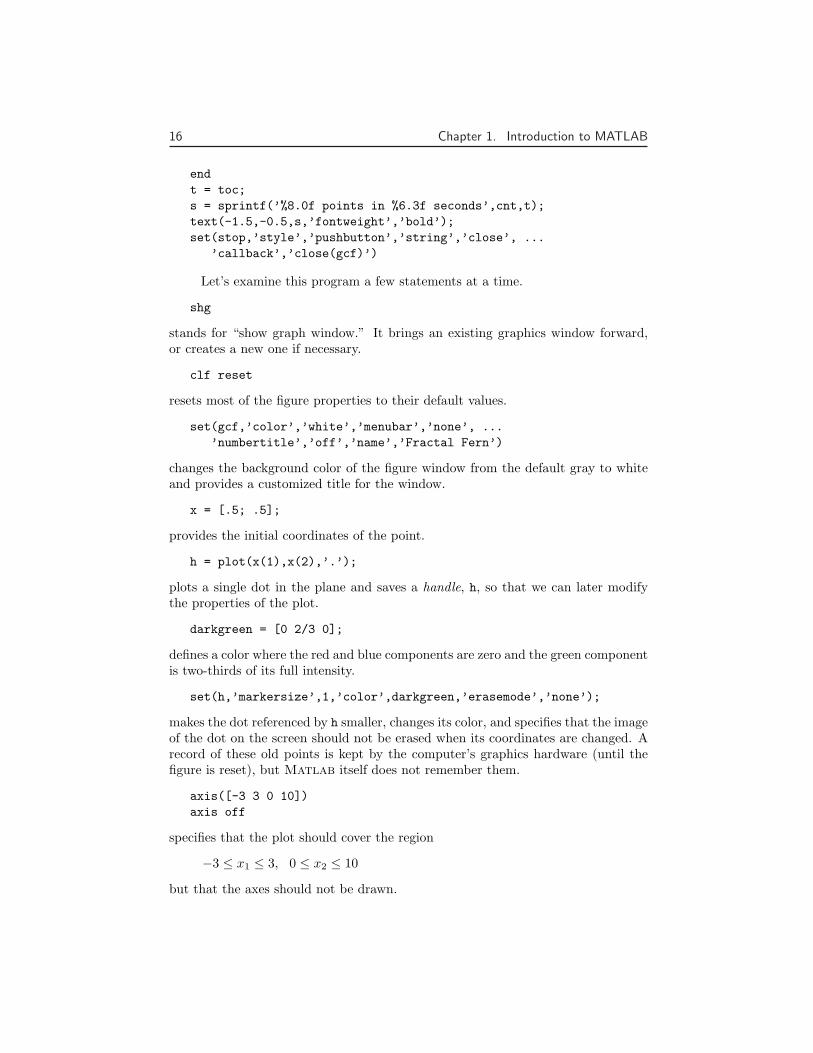
16 Chapter 1. Introduction to MATLAB
endt = toc;s = sprintf(’%8.0f points in %6.3f seconds’,cnt,t);text(-1.5,-0.5,s,’fontweight’,’bold’);set(stop,’style’,’pushbutton’,’string’,’close’, ...
’callback’,’close(gcf)’)
Let’s examine this program a few statements at a time.
shg
stands for “show graph window.” It brings an existing graphics window forward,or creates a new one if necessary.
clf reset
resets most of the figure properties to their default values.
set(gcf,’color’,’white’,’menubar’,’none’, ...’numbertitle’,’off’,’name’,’Fractal Fern’)
changes the background color of the figure window from the default gray to whiteand provides a customized title for the window.
x = [.5; .5];
provides the initial coordinates of the point.
h = plot(x(1),x(2),’.’);
plots a single dot in the plane and saves a handle, h, so that we can later modifythe properties of the plot.
darkgreen = [0 2/3 0];
defines a color where the red and blue components are zero and the green componentis two-thirds of its full intensity.
set(h,’markersize’,1,’color’,darkgreen,’erasemode’,’none’);
makes the dot referenced by h smaller, changes its color, and specifies that the imageof the dot on the screen should not be erased when its coordinates are changed. Arecord of these old points is kept by the computer’s graphics hardware (until thefigure is reset), but Matlab itself does not remember them.
axis([-3 3 0 10])axis off
specifies that the plot should cover the region
−3 ≤ x1 ≤ 3, 0 ≤ x2 ≤ 10
but that the axes should not be drawn.

1.3. Fractal Fern 17
stop = uicontrol(’style’,’toggle’,’string’,’stop’, ...’background’,’white’);
creates a toggle user interface control, labeled ’stop’ and colored white, in thedefault position near the lower left corner of the figure. The handle for the controlis saved in the variable stop.
drawnow
causes the initial figure, including the initial point, to actually be plotted on thecomputer screen.
The statement
p = [ .85 .92 .99 1.00];
sets up a vector of probabilities. The statements
A1 = [ .85 .04; -.04 .85]; b1 = [0; 1.6];A2 = [ .20 -.26; .23 .22]; b2 = [0; 1.6];A3 = [-.15 .28; .26 .24]; b3 = [0; .44];A4 = [ 0 0 ; 0 .16];
define the four affine transformations. The statements
cnt = 1;
initializes a counter that keeps track of the number of points plotted.
tic
initializes a stopwatch timer.
while ~get(stop,’value’)
begins a while loop that runs as long as the ’value’ property of the stop toggleis equal to zero. Clicking the stop toggle changes the value from zero to one andterminates the loop.
r = rand;
generates a pseudorandom value between zero and one. The compound if statement
if r < p(1)x = A1*x + b1;
elseif r < p(2)x = A2*x + b2;
elseif r < p(3)x = A3*x + b3;
elsex = A4*x;
end
18 Chapter 1. Introduction to MATLAB
picks one of the four affine transformations. Because p(1) is 0.85, the first trans-formation is chosen eighty-five percent of the time. The other three transformationsare chosen relatively infrequently.
set(h,’xdata’,x(1),’ydata’,x(2));
changes the coordinates of the point h to the new (x1, x2) and plots this new point.But, get(h,’erasemode’) is ’none’, so the old point also remains on the screen.
cnt = cnt + 1;
counts one more point.
drawnow
tells Matlab to take the time to redraw the figure, showing the new point alongwith all the old ones. Without this command nothing would be plotted until stopis toggled.
end
matches the while at the beginning of the loop. Finally
t = toc;
reads the timer.
s = sprintf(’%8.0f points in %6.3f seconds’,cnt,t);text(-1.5,-0.5,s,’fontweight’,’bold’);
displays the elapsed time since tic was called, and the final count of the numberof points plotted. Finally,
set(stop,’style’,’pushbutton’,’string’,’close’, ...’callback’,’close(gcf)’)
changes the uicontrol to a pushbutton that closes the window.
1.4 Magic SquaresMatlab stands for Matrix Laboratory. Over the years Matlab has evolved into ageneral purpose technical computing environment, but operations involving vectors,matrices, and linear algebra continue to be its most distinguishing feature.
Magic squares provide an interesting set of sample matrices. The commandshelp magic or helpwin magic tell us that
MAGIC(N) is an N-by-N matrix constructed from the integers1 through N^2 with equal row, column, and diagonal sums.Produces valid magic squares for all N > 0 except N = 2.

1.4. Magic Squares 19
Magic squares were known in China over two thousand years before the birthof Christ. The 3-by-3 magic square is known as lo-shu. Legend has it that lo-shuwas discovered on the shell of a turtle that crawled out of the Lo River in thetwenty-third century B.C. Lo-shu provides a mathematical basis for feng shui, theancient Chinese philosophy of balance and harmony. Matlab can generate lo-shuwith
A = magic(3)
which produces
A =8 1 63 5 74 9 2
The command
sum(A)
sums the elements in each column to produce
15 15 15
The command
sum(A’)’
transposes the matrix, sums the columns of the transpose, and then transposes theresults to produce the row sums
151515
The command
sum(diag(A))
sums the main diagonal of A, which runs from upper left to lower right, to produce
15
The opposite diagonal, that runs from upper right to lower left, is less important inlinear algebra, so finding its sum is a little trickier. One way to do it makes use ofthe function that “flips” a matrix “up-down”
sum(diag(flipud(A)))
produces
15
20 Chapter 1. Introduction to MATLAB
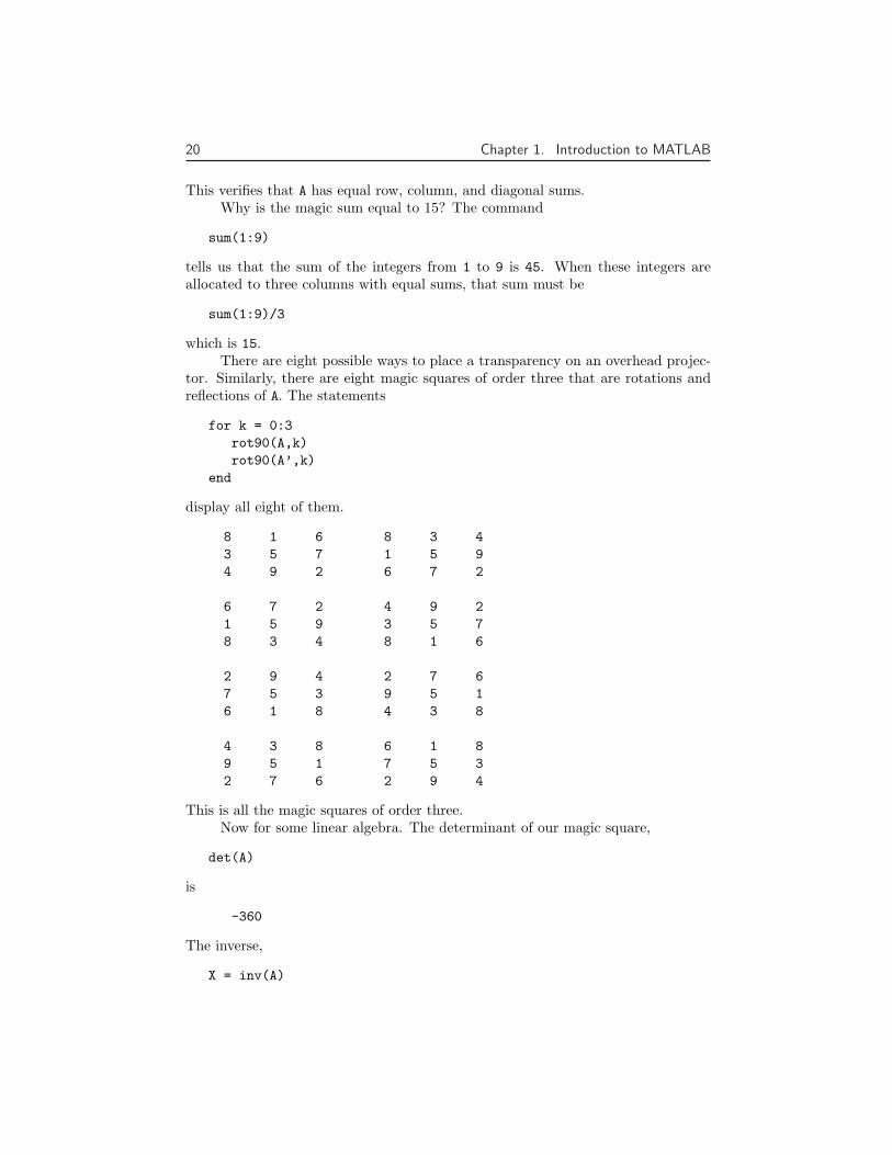
This verifies that A has equal row, column, and diagonal sums.Why is the magic sum equal to 15? The command
sum(1:9)
tells us that the sum of the integers from 1 to 9 is 45. When these integers areallocated to three columns with equal sums, that sum must be
sum(1:9)/3
which is 15.There are eight possible ways to place a transparency on an overhead projec-
tor. Similarly, there are eight magic squares of order three that are rotations andreflections of A. The statements
for k = 0:3rot90(A,k)rot90(A’,k)
end
display all eight of them.
8 1 6 8 3 43 5 7 1 5 94 9 2 6 7 2
6 7 2 4 9 21 5 9 3 5 78 3 4 8 1 6
2 9 4 2 7 67 5 3 9 5 16 1 8 4 3 8
4 3 8 6 1 89 5 1 7 5 32 7 6 2 9 4
This is all the magic squares of order three.Now for some linear algebra. The determinant of our magic square,
det(A)
is
-360
The inverse,
X = inv(A)

1.4. Magic Squares 21
is
X =0.1472 -0.1444 0.0639
-0.0611 0.0222 0.1056-0.0194 0.1889 -0.1028
The inverse looks better when it is displayed with a rational format.
format ratX
shows that the elements of X are fractions with det(A) in the denominator.
X =53/360 -13/90 23/360
-11/180 1/45 19/180-7/360 17/90 -37/360
The statement
format short
restores the output format to its default.Three other important quantities in computational linear algebra are matrix
norms, eigenvalues, and singular values. The statements
r = norm(A)e = eig(A)s = svd(A)
produce
r =15
e =15.00004.8990
-4.8990
s =15.00006.92823.4641
The magic sum occurs in all three because the vector of all ones is an eigenvector,and is also a left and right singular vector.
So far, all the computations in this section have been done using floating-pointarithmetic. This is the arithmetic used for almost all scientific and engineeringcomputation, especially for large matrices. But for a 3-by-3 matrix, it is easyto repeat the computations using symbolic arithmetic and the Symbolic Toolboxconnection to Maple. The statement

22 Chapter 1. Introduction to MATLAB
A = sym(A)
changes the internal representation of A to a symbolic form that displays as
A =[ 8, 1, 6][ 3, 5, 7][ 4, 9, 2]
Now commands like
sum(A), sum(A’)’, det(A), inv(A), eig(A), svd(A)
produce symbolic results. In particular, the eigenvalue problem for this matrix canbe solved exactly, and
e =[ 15][ 2*6^(1/2)][ -2*6^(1/2)]
A 4-by-4 magic square is one of several mathematical objects on display inMelancolia, a Renaissance etching by Albrect Durer. An electronic copy of theetching is available in a Matlab data file.
load durerwhos
produces
X 648x509 2638656 double arraycaption 2x28 112 char arraymap 128x3 3072 double array
The elements of the matrix X are indices into the gray-scale color map named map.The image is displayed with
image(X)colormap(map)axis image
Click the magnifying glass with a “+” in the toolbar and use the mouse to zoomin on the magic square in the upper right-hand corner. The scanning resolutionbecomes evident as you zoom in. The commands
load detailimage(X)colormap(map)axis image
display a higher resolution scan of the area around the magic square.The command

1.4. Magic Squares 23
A = magic(4)
produces a 4-by-4 magic square
A =16 2 3 135 11 10 89 7 6 124 14 15 1
The commands
sum(A), sum(A’), sum(diag(A)), sum(diag(flipud(A)))
produce enough 34’s to verify that A is indeed a magic square.The 4-by-4 magic square produced by Matlab is not the same as Durer’s
magic square. We need to interchange the second and third columns.
A = A(:,[1 3 2 4])
changes A to
A =16 3 2 135 10 11 89 6 7 124 15 14 1
Interchanging columns does not change the column sums or the row sums. It usuallychanges the diagonal sums, but in this case both diagonal sums are still 34. So nowour magic square matches the one in Durer’s etching. Durer probably chose thisparticular 4-by-4 square because the date he did the work, 1514, occurs in themiddle of the bottom row.
We have seen two different 4-by-4 magic squares. It turns out that there are880 different magic squares of order four and 275305224 different magic squares oforder five. Nobody knows how many different magic squares of order six or largerthere are.
The determinant of our 4-by-4 magic square, det(A), is zero. If we try tocompute its inverse
inv(A)
we get
Warning: Matrix is close to singular or badly scaled.Results may be inaccurate.
So, some magic squares represent singular matrices. Which ones? The rank of asquare matrix is the number of linearly independent rows or columns. An n-by-nmatrix is singular if and only if its rank is less than n.
The statements

24 Chapter 1. Introduction to MATLAB
for n = 1:24, r(n) = rank(magic(n)); end[(1:24)’ r’]
produce a table of order versus rank.

1.4. Magic Squares 25
1 12 23 34 35 56 57 78 39 9
10 711 1112 313 1314 915 1516 317 1718 1119 1920 321 2122 1323 2324 3
Look carefully at this table. Ignore n = 2 because magic(2) is not really a magicsquare. What patterns do you see? A bar graph makes the patterns easier to see.
bar(r)title(’Rank of magic squares’)
produces
0 5 10 15 20 250
5
10
15
20
25Rank of magic squares
26 Chapter 1. Introduction to MATLAB
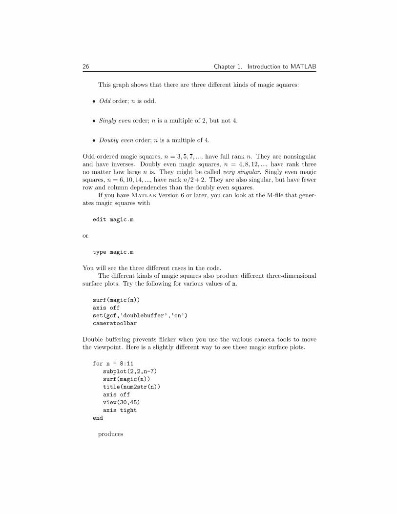
This graph shows that there are three different kinds of magic squares:
• Odd order; n is odd.
• Singly even order; n is a multiple of 2, but not 4.
• Doubly even order; n is a multiple of 4.
Odd-ordered magic squares, n = 3, 5, 7, ..., have full rank n. They are nonsingularand have inverses. Doubly even magic squares, n = 4, 8, 12, ..., have rank threeno matter how large n is. They might be called very singular. Singly even magicsquares, n = 6, 10, 14, ..., have rank n/2 + 2. They are also singular, but have fewerrow and column dependencies than the doubly even squares.
If you have Matlab Version 6 or later, you can look at the M-file that gener-ates magic squares with
edit magic.m
or
type magic.m
You will see the three different cases in the code.The different kinds of magic squares also produce different three-dimensional
surface plots. Try the following for various values of n.
surf(magic(n))axis offset(gcf,’doublebuffer’,’on’)cameratoolbar
Double buffering prevents flicker when you use the various camera tools to movethe viewpoint. Here is a slightly different way to see these magic surface plots.
for n = 8:11subplot(2,2,n-7)surf(magic(n))title(num2str(n))axis offview(30,45)axis tight
end
produces

1.5. Cryptography 27
8 9
10 11
1.5 CryptographyThis section uses a cryptography example to show how Matlab deals with text andcharacter strings. The cryptographic technique, which is known as a Hill cipher,involves arithmetic in a finite field.
Almost all modern computers use the ASCII character set to store basic text.ASCII stands for American Standard Code for Information Interchange. The char-acter set uses seven of the eight bits in a byte to encode 128 characters. The first 32characters are nonprinting control characters, such as tab, backspace and end-of-line. The 128th character is another nonprinting character that corresponds to thedelete key on your keyboard. In between these control characters are 95 printablecharacters, including a space, 10 digits, 26 lowercase letters, 26 uppercase lettersand 32 punctuation marks.
Matlab can easily display all the printable characters, in the order deter-mined by their ASCII encoding. Start with
x = reshape(32:127,32,3)’
This produces a 3-by-32 matrix.
x =32 33 34 ... 61 62 6364 65 66 ... 93 94 9596 97 98 ... 125 126 127
The char function converts numbers to characters. The statement
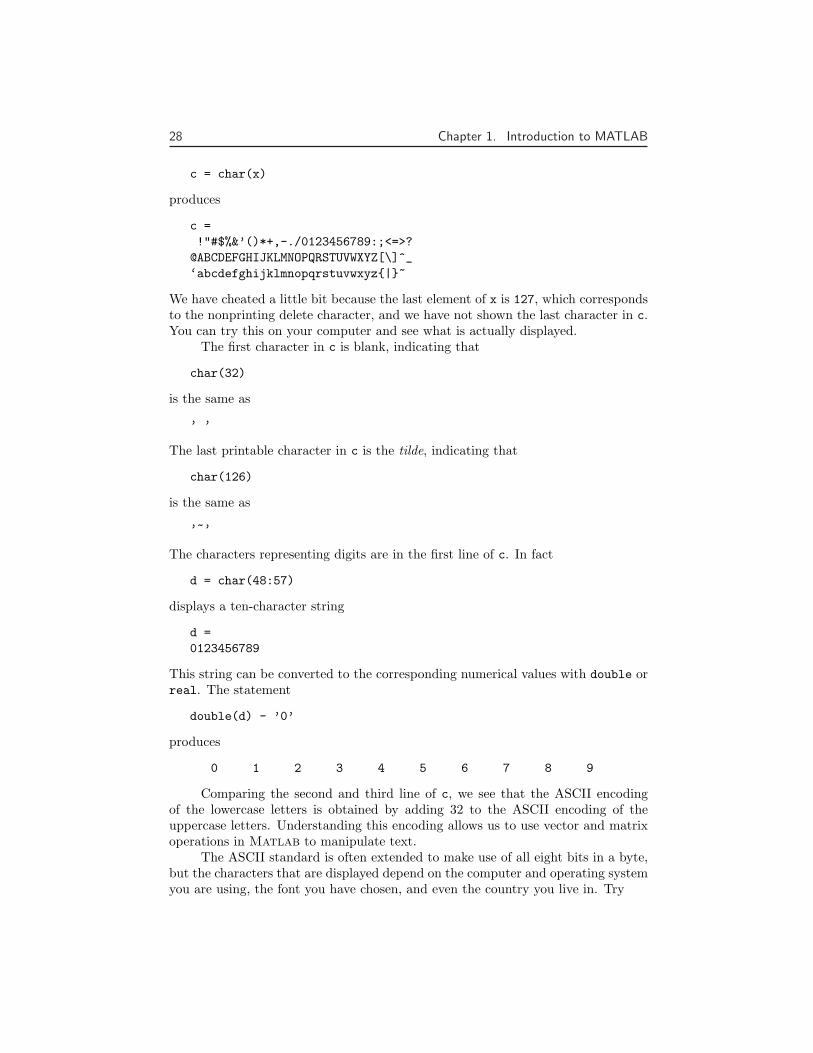
28 Chapter 1. Introduction to MATLAB
c = char(x)
produces
c =!"#$%&’()*+,-./0123456789:;<=>?
@ABCDEFGHIJKLMNOPQRSTUVWXYZ[\]^_‘abcdefghijklmnopqrstuvwxyz{|}~
We have cheated a little bit because the last element of x is 127, which correspondsto the nonprinting delete character, and we have not shown the last character in c.You can try this on your computer and see what is actually displayed.
The first character in c is blank, indicating that
char(32)
is the same as
’ ’
The last printable character in c is the tilde, indicating that
char(126)
is the same as
’~’
The characters representing digits are in the first line of c. In fact
d = char(48:57)
displays a ten-character string
d =0123456789
This string can be converted to the corresponding numerical values with double orreal. The statement
double(d) - ’0’
produces
0 1 2 3 4 5 6 7 8 9
Comparing the second and third line of c, we see that the ASCII encodingof the lowercase letters is obtained by adding 32 to the ASCII encoding of theuppercase letters. Understanding this encoding allows us to use vector and matrixoperations in Matlab to manipulate text.
The ASCII standard is often extended to make use of all eight bits in a byte,but the characters that are displayed depend on the computer and operating systemyou are using, the font you have chosen, and even the country you live in. Try

1.5. Cryptography 29
char(reshape(160:255,32,3)’)
and see what happens on your machine.Our encryption technique involves modular arithmetic. All the quantities in-
volved are integers and the result of any arithmetic operation is reduced by tak-ing the remainder or modulus with respect to a prime number, p. The functionsrem(x,y) and mod(x,y) both compute the remainder when x is divided by y. Theyproduce the same result when x and y have the same sign; the result also has thatsign. But if x and y have opposite signs, then rem(x,y) has the same sign as x,while mod(x,y) has the same sign as y. Here is a table.
x = [37 -37 37 -37]’;y = [10 10 -10 -10]’;r = [ x y rem(x,y) mod(x,y)]
produces
37 10 7 7-37 10 -7 337 -10 7 -3
-37 -10 -7 -7
We have chosen to encrypt text that uses the entire ASCII character set, notjust the letters. There are 95 such characters. The next larger prime number isp = 97, so we represent the p characters by the integers 0:p-1 and do arithmeticmod p.
The characters are encoded two at a time. Each pair of characters is repre-sented by a 2-vector, x. For example, suppose the text contains the pair of letters’TV’. The ASCII values for this pair of letters are 84 and 86. Subtracting 32 tomake the representation start at 0 produces the column vector
x =(
5254
)
The encryption is done with a 2-by-2 matrix-vector multiplication over theintegers mod p. The symbol ≡ is used to indicate that two integers have the sameremainder, modulo the specified prime.
y ≡ Ax, mod p
where A is the matrix
A =(
71 22 26
)
For our example, the product Ax is
Ax =(
38001508
)
When this is reduced mod p the result is
y =(
1753
)

30 Chapter 1. Introduction to MATLAB
Converting this back to characters by adding 32 produces ’1U’.Now comes the interesting part. Over the integers modulo p, the matrix A is
its own inverse. If
y ≡ Ax, mod p
then
x ≡ Ay, mod p
In other words, in arithmetic mod p, A2 is the identity matrix. You can check thiswith Matlab.
p = 97;A = [71 2; 2 26]I = mod(A^2,p)
produces
A =71 22 26
I =1 00 1
This means that the encryption process is its own inverse. One function can beused to both encrypt and decrypt a message.
Here is the preamble of the M-file crypto.m.
function y = crypto(x)% CRYPTO Cryptography example.% y = crypto(x) converts an ASCII text string into another% coded string. The function is its own inverse, so% crypto(crypto(x)) gives x back.% See also: ENCRYPT.
% Use a two-character Hill cipher with arithmetic% modulo 97, a prime.p = 97;
The conversion from characters to numerical values is done by
% Convert printable ASCII text to integers mod p.space = 32;delete = 127;k = find(x >= delete);x(k) = x(k)-delete;x = mod(real(x-space),p);

1.5. Cryptography 31
Prepare for the matrix-vector product by forming a matrix with two rows and lotsof columns.
% Reshape into a matrix with 2 rows and% floor(length(x)/2) columns.n = 2*floor(length(x)/2);X = reshape(x(1:n),2,n/2);
All this preparation has been so that we can do the actual finite field arithmeticquickly and easily.
% Encode with matrix multiplication modulo p.A = [71 2; 2 26];Y = mod(A*X,p);
Finally, convert the numbers back to printable characters.
% Reshape into a single row.y = reshape(Y,1,n);
% If length(x) is odd, encode the last character.if length(x) > n
y(n+1) = mod((p-1)*x(n+1),p);end
% Convert to printable ASCII characters.y = char(y+space);k = find(y >= delete);y(k) = y(k)+delete;
Let’s follow the computation of y = crypto(’Hello world’). We begin witha character string.
x = ’Hello world’
This is converted to an integer vector.
x =40 69 76 76 79 0 87 79 82 76 68
The length(x) is odd, so the reshaping temporarily ignores the last element.
X =40 76 79 87 8269 76 0 79 76
A conventional matrix-vector multiplication A*X produces an intermediate matrix.
2978 5548 5609 6335 59741874 2128 158 2228 2140
32 Chapter 1. Introduction to MATLAB
Then the mod(.,p) operation produces
Y =68 19 80 30 5731 91 61 94 6
This is rearranged to a row vector.
y =68 31 19 91 80 61 30 94 57 6
Now the last element of x is encoded by itself and attached to the end of y.
y =68 31 19 91 80 61 30 94 57 6 29
Finally, y is converted back to a character string to produce the encrypted result.
y = ’d?3{p]>~Y&=’
If we now compute crypto(y), we get back our original ’Hello world’.
1.6 The 3n + 1 sequenceHere is a famous unsolved problem in number theory. Start with any positive integern. Repeat the following steps:
• If n = 1, stop.
• If n is even, replace it with n/2.
• If n is odd, replace it with 3n + 1.
For example, starting with n = 7 produces
7, 22, 11, 34, 17, 52, 26, 13, 40, 20, 10, 5, 16, 8, 4, 2, 1
The sequence terminates after 17 steps. Note that whenever n reaches a power of2, the sequence terminates in log2 n more steps.
The unanswered question is, does the process always terminate? Or, is theresome starting value that causes the process to go on forever, either because thenumbers get larger and larger, or because some periodic cycle is generated?
This problem is known as the 3n + 1 problem. It has been studied by manyeminent mathematicians, including Collatz, Ulam, and Kakatani. A survey paperby Jeffrey Lagarias was published in the American Mathematical Monthly, Vol. 92(1985), pp. 3-23. The paper is also available on the Web at
http://www.cecm.sfu.ca/organics/papers/lagarias
Here is a Matlab code fragment that generates the sequence starting withany specified n.

1.6. The 3n + 1 sequence 33
y = n;while n > 1
if rem(n,2)==0n = n/2;
elsen = 3*n+1;
endy = [y n];
end
We don’t know ahead of time how long the resulting vector y is going to be. Butthe statement
y = [y n];
automatically increases length(y) each time it is executed.In principle, the unsolved mathematical problem is: can this code fragment
run forever? In actual fact, floating-point roundoff error causes the calculation tomisbehave whenever 3n + 1 becomes greater than 253, but it is still interesting toinvestigate modest values of n.
Let’s embed our code fragment in a GUI. The complete function is in M-filethreenplus1.m. For example, the statement
threenplus1(7)
produces
2 4 6 8 10 12 14 161
2
4
8
16
32
52n = 7
The M-file begins with a preamble containing the function header and thehelp information.
function threenplus1(n)% ‘‘Three n plus 1’’.% Study the 3n+1 sequence.% threenplus1(n) plots the sequence starting with n.

34 Chapter 1. Introduction to MATLAB
% threenplus1 with no arguments starts with n = 1.% uicontrols decrement or increment the starting n.% Is it possible for this to run forever?
The next section of code brings the current graphics window forward and resets it.Two pushbuttons, which are the default uicontrols, are positioned near the bottomcenter of the figure at pixel coordinates [260,5] and [300,5]. Their size is 25-by-22pixels and they are labeled with ’<’ and ’>’. When either button is subsequentlypushed, the ’callback’ string is executed, calling the function recursively with acorresponding ’-1’ or ’+1’ string argument. The ’tag’ property of the currentfigure, gcf, is set to a characteristic string that prevents this section of code frombeing reexecuted on subsequent calls.
if ~isequal(get(gcf,’tag’),’3n+1’)shgclf resetuicontrol( ...
’position’,[260 5 25 22], ...’string’,’<’, ...’callback’,’threenplus1(’’-1’’)’);
uicontrol( ...’position’,[300 5 25 22], ...’string’,’>’, ...’callback’,’threenplus1(’’+1’’)’);
set(gcf,’tag’,’3n+1’);end
The next section of code sets n. If nargin, the number of input arguments, iszero, then n is set to 1. If the input argument is either of the strings from thepushbutton callbacks, then n is retrieved from the ’userdata’ field of the figureand decremented or incremented. If the input argument is not a string, then it isthe desired n. In all situations, n is saved in ’userdata’ for use on subsequentcalls.
if nargin == 0n = 1;
elseif isequal(n,’-1’)n = get(gcf,’userdata’) - 1;
elseif isequal(n,’+1’)n = get(gcf,’userdata’) + 1;
endif n < 1, n = 1; endset(gcf,’userdata’,n)
We’ve seen the next section of code before; it does the actual computation.
y = n;while n > 1

1.7. Circle Generator 35
if rem(n,2)==0n = n/2;
elsen = 3*n+1;
endy = [y n];
end
The final section of code plots the generated sequence with dots connected bystraight lines, using a logarithmic vertical scale and customized tick labels.
semilogy(y,’.-’)axis tightymax = max(y);ytick = [2.^(0:ceil(log2(ymax))-1) ymax];if length(ytick) > 8, ytick(end-1) = []; endset(gca,’ytick’,ytick)title([’n = ’ num2str(y(1))]);
1.7 Circle GeneratorHere is an algorithm that was used to plot circles on some of the first computerswith graphical displays. At the time, there was no Matlab and no floating-pointarithmetic. Programs were written in machine language and arithmetic was doneon scaled integers. The circle generating program looked something like this:
x = 32768y = 0
L: load yshift right 5 bitsadd xstore in xchange signshift right 5 bitsadd ystore in yplot x ygo to L
Why does this generate a circle? In fact, does it actually generate a circle? Thereare no trig functions, no square roots, no multiplications or divisions. It’s all donewith shifts and additions.
The key to this algorithm is the fact that the new x is used in the computationof the new y. This was convenient on computers at the time because it meant youneeded only two storage locations, one for x and one for y. But, as we shall see, itis also why the algorithm comes close to working at all.
Here is a Matlab version of the same algorithm.

36 Chapter 1. Introduction to MATLAB
h = 1/32;x = 1;y = 0;while 1
x = x + h*y;y = y - h*x;plot(x,y,’.’)drawnow
end
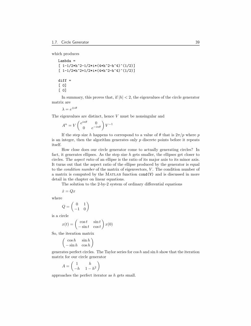
The M-file circlegen lets you experiment with various values of the step sizeh. It provides an actual circle in the background. Here is the output for the carefullychosen default value, h = .20906. It’s not quite a circle. However, circlegen(h)generates better circles with smaller values of h. Try circlegen(h) for various hyourself.
−1 −0.5 0 0.5 1
−1
−0.5
0
0.5
1
h = 0.20906
If we let (xn, yn) denote the nth point generated, then the iteration is
xn+1 = xn + hyn
yn+1 = yn − hxn+1
The key is the fact that xn+1 appears on the right in the second equation. Substi-tuting the first equation in the second gives
xn+1 = xn + hyn
yn+1 = −hxn + (1− h2)yn

1.7. Circle Generator 37
Let’s switch to matrix-vector notation. Let xn now denote the two-vectorspecifying the nth point and let A be the circle generator matrix
A =(
1 h−h 1− h2
)
With this notation, the iteration is simply
xn+1 = Axn
This immediately leads to
xn = Anx0
So, the question is, for various values of h, how do powers of the circle generatormatrix behave?
For most matrices A, the behavior of An is determined by the its eigenvalues.The Matlab statement
[V,E] = eig(A)
produces a diagonal eigenvalue matrix E and a corresponding eigenvector matrix Vso that
AV = V E
If V −1 exists, then
A = V EV −1
and
An = V EnV −1
Consequently, the powers An remain bounded if the eigenvector matrix is nonsin-gular and the eigenvalues λk, which are the diagonal elements of E, satisfy
|λk| ≤ 1
Here is an easy experiment. Enter the line
h = 2*rand, A = [1 h; -h 1-h^2], lambda = eig(A), abs(lambda)
Repeatedly press the up arrow key, then the Enter key. You should eventuallybecome convinced, at least experimentally, that
For any h in the interval 0 < h < 2, the eigenvalues of the circle generatormatrix A are complex numbers with absolute value 1.
The Symbolic Toolbox provides some assistance in actually proving this fact.
syms hA = [1 h; -h 1-h^2]lambda = eig(A)

38 Chapter 1. Introduction to MATLAB
creates a symbolic version of the iteration matrix and finds its eigenvalues.
A =[ 1, h][ -h, 1-h^2]
lambda =[ 1-1/2*h^2+1/2*(-4*h^2+h^4)^(1/2)][ 1-1/2*h^2-1/2*(-4*h^2+h^4)^(1/2)]
The statement
abs(lambda)
does not do anything useful, in part because we have not yet made any assumptionsabout the symbolic variable h.
We note that the eigenvalues will be complex whenever the quantity involvedin the square root is negative, that is, when |h| < 2. The determinant of a matrixshould be the product of its eigenvalues. This is confirmed with
d = det(A)
or
d = simple(prod(lambda))
Both produce
d =1
Consequently, when |h| < 2, the eigenvalues, λ, are complex and their product is 1,so they must satisfy |λ| = 1.
Because
λ = 1− h2/2± h√−1 + h2/4
it is plausible that, if we define θ by
cos θ = 1− h2/2
or
sin θ = h√
1− h2/4
then
λ = cos θ ± i sin θ
The Symbolic Toolbox confirms this with
theta = acos(1-h^2/2);Lambda = [cos(theta)-i*sin(theta); cos(theta)+i*sin(theta)]diff = simple(lambda-Lambda)
1.7. Circle Generator 39
which produces
Lambda =[ 1-1/2*h^2-1/2*i*(4*h^2-h^4)^(1/2)][ 1-1/2*h^2+1/2*i*(4*h^2-h^4)^(1/2)]
diff =[ 0][ 0]
In summary, this proves that, if |h| < 2, the eigenvalues of the circle generatormatrix are
λ = e±iθ
The eigenvalues are distinct, hence V must be nonsingular and
An = V
(einθ 00 e−inθ
)V −1
If the step size h happens to correspond to a value of θ that is 2π/p where pis an integer, then the algorithm generates only p discrete points before it repeatsitself.
How close does our circle generator come to actually generating circles? Infact, it generates ellipses. As the step size h gets smaller, the ellipses get closer tocircles. The aspect ratio of an ellipse is the ratio of its major axis to its minor axis.It turns out that the aspect ratio of the ellipse produced by the generator is equalto the condition number of the matrix of eigenvectors, V . The condition number ofa matrix is computed by the Matlab function cond(V) and is discussed in moredetail in the chapter on linear equations.
The solution to the 2-by-2 system of ordinary differential equations
x = Qx
where
Q =(
0 1−1 0
)
is a circle
x(t) =(
cos t sin t− sin t cos t
)x(0)
So, the iteration matrix(cosh sin h− sin h cosh
)
generates perfect circles. The Taylor series for cos h and sin h show that the iterationmatrix for our circle generator
A =(
1 h−h 1− h2
)
approaches the perfect iterator as h gets small.

40 Chapter 1. Introduction to MATLAB
1.8 Floating PointsSome people believe that
• Numerical analysis is the study of floating-point arithmetic.
• Floating-point arithmetic is unpredictable and hard to understand.
We intend to convince you that both of these assertions are false. Very little ofthis book is actually about floating-point arithmetic. But when the subject doesarise, we hope you will find floating-point arithmetic is not only computationallypowerful, but also mathematically elegant.
If you look carefully at the definitions of fundamental arithmetic operationslike addition and multiplication, you soon encounter the mathematical abstractionknown as the real numbers. But actual computation with real numbers is not verypractical because it involves limits and infinities. Instead, Matlab and most othertechnical computing environments use floating-point arithmetic, which involves afinite set of numbers with finite precision. This leads to the phenomena of roundofferror, underflow, and overflow. Most of the time, it is possible to use Matlabeffectively without worrying about these details, but every once in a while, it paysto know something about the properties and limitations of floating-point numbers.
Twenty years ago, the situation was far more complicated than it is today.Each computer had its own floating-point number system. Some were binary; somewere decimal. There was even a Russian computer that used trinary arithmetic.Among the binary computers, some used 2 as the base; others used 8 or 16. Andeverybody had a different precision. In 1985, the IEEE Standards Board and theAmerican National Standards Institute adopted the ANSI/IEEE Standard 754-1985for Binary Floating-Point Arithmetic. This was the culmination of almost a decadeof work by a 92-person working group of mathematicians, computer scientists, andengineers from universities, computer manufacturers, and microprocessor compa-nies.
All computers designed since 1985 use IEEE floating-point arithmetic. Thisdoesn’t mean that they all get exactly the same results, because there is someflexibility within the standard. But it does mean that we now have a machine-independent model of how floating-point arithmetic behaves.
Matlab uses the IEEE double-precision format. There is also a single-precision format that saves space but isn’t much faster on modern machines. And,there is an extended precision format, which is optional and therefore is one of thereasons for lack of uniformity among different machines.
Most nonzero floating-point numbers are normalized. This means they can beexpressed as
x = ±(1 + f) · 2e
where f is the fraction or mantissa and e is the exponent. The fraction satisfies
0 ≤ f < 1
1.8. Floating Points 41
and must be representable in binary using at most 52 bits. In other words, 252f isan integer in the interval
0 ≤ 252f < 252
The exponent e is an integer in the interval
−1022 ≤ e ≤ 1023
The finiteness of f is a limitation on precision. The finiteness of e is a limitationon range. Any numbers that don’t meet these limitations must be approximatedby ones that do.
Double precision floating-point numbers can be stored in a 64 bit word, with52 bits for f , 11 bits for e, and one bit for the sign of the number. The sign of eis accommodated by storing e + 1023, which is between 1 and 211 − 2. The twoextreme values for the exponent field, 0 and 211 − 1, are reserved for exceptionalfloating-point numbers that we will describe later.
The entire fractional part of a floating-point number is not f , but 1+f , whichhas 53 bits. However the leading 1 doesn’t need to be stored. In effect, the IEEEformat packs 65 bits of information into a 64 bit word.
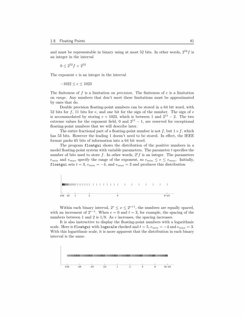
The program floatgui shows the distribution of the positive numbers in amodel floating-point system with variable parameters. The parameter t specifies thenumber of bits used to store f . In other words, 2tf is an integer. The parametersemin and emax specify the range of the exponent, so emin ≤ e ≤ emax. Initially,floatgui sets t = 3, emin = −4, and emax = 3 and produces this distribution
1/16 1/2 1 2 4 8−1/2
||||||||||||||||||||||||| | | | | | | | | | | | | | | | | | | | | | | | | | | | | | | |
Within each binary interval, 2e ≤ x ≤ 2e+1, the numbers are equally spaced,with an increment of 2e−t. When e = 0 and t = 3, for example, the spacing of thenumbers between 1 and 2 is 1/8. As e increases, the spacing increases.
It is also instructive to display the floating-point numbers with a logarithmicscale. Here is floatgui with logscale checked and t = 5, emin = −4 and emax = 3.With this logarithmic scale, it is more apparent that the distribution in each binaryinterval is the same.
1/16 1/8 1/4 1/2 1 2 4 8 16−1/4
||||||||||||||||||||||||||||||||||||||||||||||||||||||||||||||||||||||||||||||||||||||||||||||||||||||||||||||||||||||||||||||||||||||||||||||||||||||||||||||||||||||||||||||||||||||||||||||||||||||||||||||||||||||||||||||||||||||||||||||||||||||||||||||||
42 Chapter 1. Introduction to MATLAB
A very important quantity associated with floating-point arithmetic is high-lighted in red by floatgui. Matlab calls this quantity eps, which is short formachine epsilon.
eps is the distance from 1 to the next larger floating-point number.
For the floatgui model floating-point system, eps = 2^(-t).Before the IEEE standard, different machines had different values of eps.
Now, for IEEE double-precision,
eps = 2^(-52)
The approximate decimal value of eps is 2.2204 ·10−16. Either eps/2 or eps can becalled the roundoff level. The maximum relative error incurred when the result ofan arithmetic operation is rounded to the nearest floating-point number is eps/2.The maximum relative spacing between numbers is eps. In either case, you can saythat the roundoff level is about 16 decimal digits.
A frequent instance of roundoff error occurs with the simple Matlab state-ment
t = 0.1
The value stored in t is not exactly 0.1 because expressing the decimal fraction1/10 in binary requires an infinite series. In fact,
110
=124
+125
+026
+027
+128
+129
+0
210+
0211
+1
212+ ...
After the first term, the sequence of coefficients 1, 0, 0, 1 is repeated infinitely often.The floating-point number nearest 0.1 is obtained by terminating this series after53 terms. The infinite series beginning with the 54th term is larger than half a unitin the 53rd place, so the the last four coefficients are rounded up to binary 1010.Grouping the resulting terms together four at a time expresses the approximationas a base 16, or hexadecimal, series. So the resulting value of t is actually
t = (1 +916
+9
162+
9163
+ ... +9
1612+
101613
) · 2−4
The Matlab command
format hex
causes t to be displayed as
3fb999999999999a
The characters a through f represent the hexadecimal “digits” 10 through 15. Thefirst three characters, 3fb, give the hexadecimal representation of decimal 1019,which is the value of the biased exponent, e + 1023, when e is −4. The other 13characters are the hex representation of the fraction f .
In summary, the value stored in t is very close to, but not exactly equal to,0.1. The distinction is occasionally important. For example, the quantity

1.8. Floating Points 43
0.3/0.1
is not exactly equal to 3 because the actual numerator is a little less than 0.3 andthe actual denominator is a little greater than 0.1.
Ten steps of length t are not precisely the same as one step of length 1.Matlab is careful to arrange that the last element of the vector
0:0.1:1
is exactly equal to 1, but if you form this vector yourself by repeated additions of0.1, you will miss hitting the final 1 exactly.
What does the floating-point approximation to the golden ratio look like?
format hexphi = (1 + sqrt(5))/2
produces
phi =3ff9e3779b97f4a8
The first hex digit, 3, is 0011 in binary. The first bit is the sign of the floating-point number; 0 is positive, 1 is negative. So phi is positive. The remaining bitsof the first three hex digits contain e + 1023. In this example, 3ff in base 16 is3 · 162 + 15 · 16 + 15 = 1023 in decimal. So
e = 0
In fact, any floating-point number between 1.0 and 2.0 has e = 0, so its hex outputbegins with 3ff. The other 13 hex digits contain f . In this example,
f =916
+14162
+3
163+ ... +
101612
+8
1613
With these values of f and e
(1 + f)2e ≈ φ
Another example is provided by the following code segment.
format longx = 4/3 - 1y = 3*xz = 1 - y
The output produced is
x =0.33333333333333
y =1.00000000000000
z =2.220446049250313e-016
44 Chapter 1. Introduction to MATLAB
With exact computation, z would be 0. But in floating-point, the computed z isactually equal to eps. It turns out that the only roundoff error occurs in divisionin the first statement. The quotient cannot be exactly 4/3, except on that Russiantrinary computer. Consequently the value stored in x is close to, but not exactlyequal to, 1/3. Moreover, its last bit is zero. This means that the multiplication 3*xcan be done without any roundoff error. The value stored in y is not exactly equalto 1 and so the value stored in z is not 0. Before the IEEE standard, this code wasused as a quick way to estimate the roundoff level on various computers.
The roundoff level eps is sometimes called floating-point zero, but that’s amisnomer. There are many floating-point numbers much smaller than eps. Thesmallest positive normalized floating-point number has f = 0 and e = −1022. Thelargest floating-point number has f a little less than 1 and e = 1023. Matlabcalls these numbers realmin and realmax. Together with eps, they characterizethe standard system.
Binary Decimaleps 2^(-52) 2.2204e-16realmin 2^(-1022) 2.2251e-308realmax (2-eps)*2^1023 1.7977e+308
When any computation tries to produce a value larger than realmax, it is saidto overflow. The result is an exceptional floating-point value called infinity or Inf.It is represented by taking e = 1024 and f = 0 and satisfies relations like 1/Inf =0 and Inf+Inf = Inf.
When any computation tries to produce a value that is undefined even in thereal number system, the result is an exceptional value known as Not-a-Number, orNaN. Examples include 0/0 and Inf-Inf. NaN is represented by taking e = 1024and f nonzero.
When any computation tries to produce a value smaller than realmin, it issaid to underflow. This involves one of the optional, and controversial, aspects ofthe IEEE standard. Many, but not all, machines allow exceptional denormal or sub-normal floating-point numbers in the interval between realmin and eps*realmin.The smallest positive subnormal number is about 0.494e-323. Any results smallerthan this are set to zero. On machines without subnormals, any results less thanrealmin are set to zero. The subnormal numbers fill in the gap you can see inthe floatgui model system between zero and the smallest positive number. Theydo provide an elegant way to handle underflow, but their practical importance forMatlab style computation is very rare. Denormal numbers are represented bytaking e = −1023, so the biased exponent e + 1023 is zero.
Matlab uses the floating-point system to handle integers. Mathematically,the numbers 3 and 3.0 are the same, but many programming languages would usedifferent representations for the two. Matlab does not distinguish between them.We sometimes use the term flint to describe a floating-point number whose value isan integer. Floating-point operations on flints do not introduce any roundoff error,as long as the results are not too large. Addition, subtraction, and multiplication offlints produce the exact flint result, if it is not larger than 253. Division and squareroot involving flints also produce a flint when the result is an integer. For example,

1.8. Floating Points 45
sqrt(363/3) produces 11, with no roundoff error.Two Matlab functions that take apart and put together floating point num-
bers are log2 and pow2.
help log2help pow2
produces
[F,E] = LOG2(X) for each element of the real array X,returns an array F of real numbers, usually in the range0.5 <= abs(F) < 1, and an array E of integers, so thatX = F .* 2.^E. Any zeros in X produce F = 0 and E = 0.
X = POW2(F,E) for each element of the real array F andan integer array E computes X = F .* (2 .^ E). The resultis computed quickly by simply adding E to the floatingpoint exponent of F.
The quantities F and E used by log2 and pow2 predate the IEEE floating-pointstandard and so are slightly different from the f and e we are using in this section.In fact, f = 2*F-1 and e = E-1.
[F,E] = log2(phi)
produces
F =0.80901699437495
E =1
Then
phi = pow2(F,E)
gives back
phi =1.61803398874989
As an example of how roundoff error affects matrix computations, considerthe two-by-two set of linear equations
17x1 + 5x2 = 221.7x1 + 0.5x2 = 2.2
The obvious solution is x1 = 1, x2 = 1. But the Matlab statements
A = [17 5; 1.7 0.5]b = [22; 2.2]x = A\b

46 Chapter 1. Introduction to MATLAB
produce
x =-1.05888.0000
Where did this come from? Well, the equations are singular, but consistent. Thesecond equation is just 0.1 times the first. The computed x is one of infinitelymany possible solutions. But the floating-point representation of the matrix A isnot exactly singular because A(2,1) is not exactly 17/10.
The solution process subtracts a multiple of the first equation from the second.The multiplier is mu = 1.7/17, which turns out to be the floating-point numberobtained by truncating, rather than rounding, the binary expansion of 1/10. Thematrix A and the right-hand side b are modified by
A(2,:) = A(2,:) - mu*A(1,:)b(2) = b(2) - mu*b(1)
With exact computation, both A(2,2) and b(2) would become zero, but withfloating-point arithmetic, they both become nonzero multiples of eps.
A(2,2) = (1/4)*eps= 5.5511e-17
b(2) = 2*eps= 4.4408e-16
Matlab notices the tiny value of the new A(2,2) and displays a messagewarning that the matrix is close to singular. It then computes the solution of themodified second equation by dividing one roundoff error by another.
x(2) = b(2)/A(2,2)= 8
This value is substituted back into the first equation to give
x(1) = (22 - 5*x(2))/17= -1.0588
The details of the roundoff error lead Matlab to pick out one particular solutionfrom among the infinitely many possible solutions to the singular system.
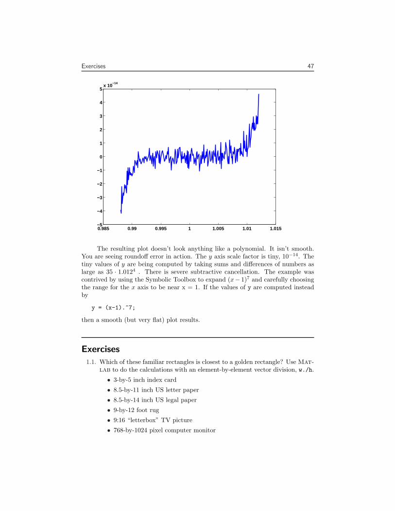
Our final example plots a seventh degree polynomial.
x = 0.988:.0001:1.012;y = x.^7-7*x.^6+21*x.^5-35*x.^4+35*x.^3-21*x.^2+7*x-1;plot(x,y)
Exercises 47
0.985 0.99 0.995 1 1.005 1.01 1.015−5
−4
−3
−2
−1
0
1
2
3
4
5x 10
−14
The resulting plot doesn’t look anything like a polynomial. It isn’t smooth.You are seeing roundoff error in action. The y axis scale factor is tiny, 10−14. Thetiny values of y are being computed by taking sums and differences of numbers aslarge as 35 · 1.0124 . There is severe subtractive cancellation. The example wascontrived by using the Symbolic Toolbox to expand (x− 1)7 and carefully choosingthe range for the x axis to be near x = 1. If the values of y are computed insteadby
y = (x-1).^7;
then a smooth (but very flat) plot results.
Exercises1.1. Which of these familiar rectangles is closest to a golden rectangle? Use Mat-
lab to do the calculations with an element-by-element vector division, w./h.
• 3-by-5 inch index card
• 8.5-by-11 inch US letter paper
• 8.5-by-14 inch US legal paper
• 9-by-12 foot rug
• 9:16 “letterbox” TV picture
• 768-by-1024 pixel computer monitor

48 Chapter 1. Introduction to MATLAB
1.2. ISO standard A4 paper is commonly used throughout the world, except inthe United States. Its dimensions are 210 by 297 millimeters. This is not agolden rectangle, but the aspect ratio is close to another familiar irrationalmathematical quantity. What is that quantity? If you fold a piece of A4paper in half, what is the aspect ratio of each of the halves? Modify theM-file goldrect.m to illustrate this property.
1.3. How many terms in the truncated continued fraction does it take to approx-imate φ with an error less than 10−10? As the number of terms increasesbeyond this, roundoff error eventually intervenes. What is the best accuracyyou can hope to achieve with double-precision floating-point arithmetic andhow many terms does it take?
1.4. Use the Matlab backslash operator to solve the 2-by-2 system of simultane-ous linear equations
c1 + c2 = 1c1φ + c2(1− φ) = 1
for c1 and c2. You can find out about the backslash operator by taking apeek at the next chapter of this book, or with the commands
help \help slash
1.5. The statement
semilogy(fibonacci(18),’-o’)
makes a logarithmic plot of Fibonacci numbers versus their index. The graphis close to a straight line. What is the slope of this line?
1.6. How does the execution time of fibnum(n) depend on the execution timefor fibnum(n-1) and fibnum(n-2)? Use this relationship to obtain an ap-proximate formula for the execution time of fibnum(n) as a function of n.Estimate how long it would take your computer to compute fibnum(50).Warning: you probably do not want to actually run fibnum(50).
1.7. What is the index of the largest Fibonacci number that can be representedexactly as a Matlab double-precision quantity without roundoff error? Whatis the index of the largest Fibonacci number that can be represented approx-imately as a Matlab double-precision quantity without overflowing?
1.8. Enter the statements
A = [1 1; 1 0]X = [1 0; 0 1]
Then enter the statement
X = A*X
Now repeatedly press the up arrow key, followed by the Enter key. Whathappens? Do you recognize the matrix elements being generated? How manytimes would you have to repeat this iteration before X overflows?

Exercises 49
1.9. Change the fern color scheme to use pink on a black background. Don’t forgetthe stop button.
1.10. What happens if you resize the figure window while the fern is being gener-ated? Why?
1.11. Flip the fern by interchanging its x and y coordinates.1.12. What happens to the fern if you change the only nonzero element in the
matrix A4?1.13. In the following statements, change how often to some reasonable value and
insert the statements in appropriate places in fern.m.
htitle = title(’0’);
if rem(cnt,how_often) == 0set(htitle,’string’,num2str(cnt))
end
1.14. What are the coordinates of the lower end of the fern’s stem?1.15. The coordinates of the point at the upper tip end of the fern can be computed
by solving a certain 2-by-2 system of simultaneous linear equations. What isthat system and what are the coordinates of the tip?
1.16. The M-file finitefern.m can be used to produce printed output of the fern.Explain why printing is possible with finitefern.m, but not with fern.m.
1.17. The fern algorithm involves repeated random choices from four differentformulas for advancing the point. When the kth formula is used repeat-edly by itself, without random choices, it defines a deterministic trajectory,Tk, k = 1, ..., 4, in the (x, y) plane. Modify finitefern.m so that plots ofeach of these four trajectories are superimposed on the plot of the fern. Eachtrajectory starts at ( 1
2 , 12 ) and approaches some limit point, zk. Compute
these limit points and plot a ’o’ there. You can superimpose several plotswith
plot(...)hold onplot(...)plot(...)hold off
1.18. Modify fern.m or finitefern.m so that it produces Sierpinski’s triangle.Start at
x =(
1/21/2
)
At each iterative step the current point x is replaced by Ax + b where thematrix A is always
A =(
1/2 00 1/2
)
50 Chapter 1. Introduction to MATLAB
and the vector b is chosen at random with equal probability from among thethree vectors
b =(
1/20
), b =
(0
1/2
), or b =
(00
)
1.19. A = magic(4) is singular. Its columns are linearly dependent. What donull(A), null(A,’r’), null(sym(A)), and rref(A) tell you about that de-pendence?
1.20. Let A = magic(n) for n = 3, 4, or 5. What does
p = randperm(n); q = randperm(n); A = A(p,q);
do to
sum(A)sum(A’)’sum(diag(A))sum(diag(flipud(A)))rank(A)
1.21. The character char(7) is a control character. What does it do?1.22. What does char([169 174]) display on your machine?1.23. What fundamental physical law is hidden in this string?
s = ’/b_t3{$H~MO6JTQI>v~#3Gieyjl(p,nF’
You should be able to enter most of the string with a cut and paste operation.Then set
s(25) = char(255)
1.24. Find the two files encrypt.m and gettysburg.dat. Use encrypt to encryptgettysburg.dat. Then decrypt the result. Use encrypt to encrypt itself.
1.25. If x is the character string consisting of just two blanks,
x = ’ ’
then crypto(x) is actually equal to x. Why does this happen? Are thereany other two-character strings that crypto does not change?
1.26. Find another 2-by-2 integer matrix A for which
mod(A*A,97)
is the identity matrix. Replace the matrix in crypto.m with your matrix andverify that the function still works correctly.
1.27. The function crypto works with 97 characters instead of 95, so it can pro-duce output, and correctly handle input, that contains two characters withASCII values greater than 127. What are these characters? Choose two othercharacters in the extended set and change crypto to use these two instead.
Exercises 51
1.28. Create a new crypto function that works with just 29 characters, the 26lowercase letters, plus blank, period, and comma. You will need to find a2-by-2 integer matrix A for which mod(A*A,29) is the identity matrix.
1.29. The graph of the 3n + 1 sequence has a particular characteristic shape if thestarting n is 5, 10, 20, 40, . . ., that is, n is five times a power of two. What isthis shape and why does it happen?
1.30. The graphs of the 3n+1 sequences starting at n = 108, 109, and 110 are verysimilar to each other. Why?
1.31. Let L(n) be the number of terms in the 3n + 1 sequence that starts with n.Write a Matlab function that computes L(n) without using any vectors orunpredictable amounts of storage. Plot L(n) for 1 ≤ n ≤ 1000. What is themaximum value of L(n) for n in this range, and for what value of n does itoccur? Use threenplus1 to plot the sequence that starts with this particularvalue of n.
1.32. How was the default value of the step size h for circlegen chosen?1.33. Modify circlegen so that both components of the new point are determined
from the old point, that is,
xn+1 = xn + hyn
yn+1 = yn − hxn
(This is the explicit Euler’s method for solving the circle ordinary differentialequation.) What happens to the “circles”? What is the iteration matrix?What are its eigenvalues?Modify circlegen so that the new point is determined by solving a 2-by-2system of simultaneous equations.
xn+1 − hyn+1 = xn
yn+1 + hxn+1 = yn
(This is the implicit Euler’s method for solving the circle ordinary differentialequation.) What happens to the “circles”? What is the iteration matrix?What are its eigenvalues?
1.34. Modify circlegen so that it keeps track of the maximum and minimumradius during the iteration and returns the ratio of these two radii as the valueof the function. Compare this computed aspect ratio with the eigenvectorcondition number, cond(V), for various values of h.
1.35. What happens with circlegen(sqrt(2))? (Don’t answer too quickly.)1.36. Modify circlegen so that you can investigate the behavior of the circle-
generating algorithm for√
2 < h < 2.1.37. What is the circle generator iteration matrix A when h = 2? How does An
behave? Can you explain this behavior using just the eigenvalues of A? Whatis the condition number of the eigenvector matrix, V ?
1.38. What happens with the circle-generating algorithm when h > 2?1.39. Modify floatgui.m by changing its last line from a comment to an executable
statement and changing the question mark to a simple expression that counts

52 Chapter 1. Introduction to MATLAB
the number of floating-point numbers in the model system.1.40. Explain the output produced by
t = 0.1n = 1:10e = n/10 - n*t
1.41. What does each of these programs do? How many lines out output does eachprogram produce? What are the last two values of x printed?
x = 1; while 1+x > 1, x = x/2, pause(.02), end
x = 1; while x+x > x, x = 2*x, pause(.02), end
x = 1; while x+x > x, x = x/2, pause(.02), end
1.42. Which familiar real numbers are approximated by floating-point numbersthat display the following values with format hex?
40590000000000003f847ae147ae147b3fe921fb54442d18
1.43. Let F be the set of all IEEE double precision floating point numbers, exceptNaNs and Infs, which have biased exponent 7ff(hex), and denormals, whichhave biased exponent 000(hex).(a) How many elements are there in F?(b) What fraction of the elements of F are in the interval 1 <= x < 2?(c) What fraction of the elements of F are in the interval 1/64 <= x < 1/32?(d) Determine by random sampling approximately what fraction of the ele-ments x of F satisfy the Matlab logical relation
x*(1/x) == 1
1.44. The classic quadratic formula says that the two roots of the quadratic equa-tion
ax2 + bx + c = 0
are
x1, x2 =−b±√b2 − 4ac
2a
Use this formula in Matlab to compute both roots when
a = 1, b = −100000000, c = 1
Compare your computed results with
roots([a b c])
Exercises 53
What happens if you try to compute the roots by hand or with a handcalculator?You should find that the classic formula is good for computing one root, butnot the other. So use it to compute one root accurately and then use the factthat
x1x2 =c
a
to compute the other.1.45. The power series for sin x is
sin x = x− x3
3!+
x5
5!− x7
7!+ ...
Here is a Matlab function that uses this series to compute sin x.
function s = powersin(x)% POWERSIN. Power series for sin(x).% POWERSIN(x) tries to compute sin(x) from a power seriess = 0;t = x;n = 1;while s+t ~= s;
s = s + t;t = -x.^2/((n+1)*(n+2)).*t;n = n + 2;
end
What causes the while loop to terminate?Answer each of the following questions for x = π/2, 11π/2, 21π/2, and 31π/2:
How accurate is the computed result?
How many terms are required?
What is the largest term in the series?
What do you conclude about the use of floating-point arithmetic and powerseries to evaluate functions?
1.46. In the Gregorian calendar, a year y is a leap year if and only if
(mod(y,4) == 0) & (mod(y,100) ~= 0) | (mod(y,400) == 0)
Thus, 2000 was a leap year, but 2100 will not be a leap year. This rule impliesthat the Gregorian calendar repeats itself every 400 years. In that 400 yearperiod, there are 97 leap years, 4800 months, 20871 weeks and 146097 days.The Matlab functions datenum, datevec, datestr, and weekday use thesefacts to facilitate computations involving calendar dates. For example, eitherof the statements
[d,w] = weekday(’Aug. 17, 2002’)

54 Chapter 1. Introduction to MATLAB
or
[d,w] = weekday(datenum([2002 8 17]))
tells me that my birthday was on a Saturday in 2002..Use Matlab to answer the following questions.(a) On what day of the week were you born?(b) In a 400 year Gregorian calendar cycle, which week day is the most likelyfor your birthday?(c) What is the probability that the 13th of any month falls on a Friday?The answer is close to, but not exactly equal to, 1/7.