chapter 1 introduction to optimization - sas...

Chapter 1Introduction to Optimization

Chapter Contents

OVERVIEW . . . . . . . . . . . . . . . . . . . . . . . . . . . . . . . . . . . 15

DATA FLOW . . . . . . . . . . . . . . . . . . . . . . . . . . . . . . . . . . . 16PROC LP . . . . . . . . . . . . . . . . . . . . . . . . . . . . . . . . . . . 17PROC NETFLOW . . . . . . . . . . . . . . . . . . . . . . . . . . . . . . . 17PROC INTPOINT . . . . . . . . . . . . . . . . . . . . . . . . . . . . . . . 19PROC NLP . . . . . . . . . . . . . . . . . . . . . . . . . . . . . . . . . . 20PROC QP (Experimental) . . . . . . . . . . . . . . . . . . . . . . . . . . . 21PROC TRANS . . . . . . . . . . . . . . . . . . . . . . . . . . . . . . . . . 22PROC ASSIGN . . . . . . . . . . . . . . . . . . . . . . . . . . . . . . . . 22Model Formats: PROC LP and PROC NETFLOW . . . . . . . . . . . . . . 23Model Formats: PROC ASSIGN and PROC TRANS . . . . . . . . . . . . 33

MODEL BUILDING . . . . . . . . . . . . . . . . . . . . . . . . . . . . . . 34

MATRIX GENERATION . . . . . . . . . . . . . . . . . . . . . . . . . . . . 36Exploiting Model Structure . . . . . . . . . . . . . . . . . . . . . . . . . . 38

REPORT WRITING . . . . . . . . . . . . . . . . . . . . . . . . . . . . . . 41The DATA Step . . . . . . . . . . . . . . . . . . . . . . . . . . . . . . . . 41Other Reporting Procedures . . . . . . . . . . . . . . . . . . . . . . . . . . 43

DECISION SUPPORT SYSTEMS . . . . . . . . . . . . . . . . . . . . . . . 44The Full-Screen Interface . . . . . . . . . . . . . . . . . . . . . . . . . . . 44Communicating with the Optimization Procedures . . . . . . . . . . . . . . 45

REFERENCES . . . . . . . . . . . . . . . . . . . . . . . . . . . . . . . . . . 45

14 � Chapter 1. Introduction to Optimization

Chapter 1Introduction to Optimization

Overview

This chapter describes how to use SAS/OR software to solve a wide variety of opti-mization problems. The basic optimization problem is that of minimizing or maxi-mizing an objective function subject to constraints imposed on the variables of thatfunction. The objective function and constraints can be linear or nonlinear; the con-straints can be bound constraints, equality or inequality constraints, or integer con-straints.

Traditionally, optimization problems are divided into linear programming (LP; allfunctions are linear) and nonlinear programming (NLP). Variations of LP prob-lems are assignment problems, network flow problems, and transportation problems.Nonlinear regression (fitting a nonlinear model to a set of data and the subsequent sta-tistical analysis of the results) is a special NLP problem. Since these applications areso common, SAS/OR software has separate procedures or facilities within proceduresfor solving each type of these problems. Model data are supplied in a form suited forthe particular type of problem. Another benefit is that an optimization algorithm canbe specialized for the particular type of problem, reducing solution times. Optimizerscan exploit some structure in problems such as embedded networks, special orderedsets, least squares, and quadratic objective functions.

SAS/OR software has seven procedures used for optimization:

• PROC ASSIGN for solving assignment problems

• PROC INTPOINT for network programming problems with side constraints,and linear programming problems solved by an interior point algorithm

• PROC LP for solving linear and mixed integer programming problems

• PROC NETFLOW for solving network programming problems with side con-straints

• PROC NLP for solving nonlinear programming problems

• PROC QP for solving quadratic programming problems

• PROC TRANS for solving transportation problems

SAS/OR procedures use syntax that is similar to other SAS procedures. In particular,all SAS retrieval, data management, reporting, and analysis can be used with SAS/ORsoftware. Each optimizer is designed to integrate with the SAS System to simplifymodel building, maintenance, solution, and report writing.

Data for models are supplied to SAS/OR procedures in SAS data sets. These data setscan be saved and easily changed and the problem can be solved. Because the models


are in SAS data sets, problem data that can represent pieces of a larger model can beconcatenated and merged. The SAS/OR procedures output SAS data sets containingthe solutions. These can then be used to produce customized reports. This structureallows decision support systems to be constructed using SAS/OR procedures andother tools in the SAS System as building blocks.

The following list suggests application areas where decision support systems havebeen used. In practice, models often contain elements of several applications listedhere.

• Product-Mix problems find the mix of products that generates the largest re-turn when there are several products that compete for limited resources.

• Blending problems find the mix of ingredients to be used in a product so thatit meets minimum standards at minimum cost.

• Time-Staged problems are models whose structure repeats as a function oftime. Production and inventory models are classic examples of time-stagedproblems. In each period, production plus inventory minus current demandequals inventory carried to the next period.

• Scheduling problems assign people to times, places, or tasks so as to optimizepeople’s preferences while satisfying the demands of the schedule.

• Multiple objective problems have multiple conflicting objectives. Typically,the objectives are prioritized and the problems are solved sequentially in a pri-ority order.

• Capital budgeting and project selection problems ask for the project or setof projects that will yield the greatest return.

• Location problems seek the set of locations that meets the distribution needsat minimum cost.

• Cutting stock problems find the partition of raw material that minimizeswaste.

Data Flow

The LP, NETFLOW, INTPOINT, NLP, QP, TRANS, and ASSIGN procedures takea model that has been saved in one or more SAS data sets, solve it, and save thesolution in other SAS data sets. Most of the procedures define a SAS macro variablethat contains a character string indicating whether or not the procedure terminatedsuccessfully and the status of the optimizer (for example, whether the optimum wasfound). This information is useful when the procedure is one of the steps in a largerprogram.

PROC NETFLOW � 17

PROC LP

The LP procedure solves linear and mixed integer programs. It can perform severaltypes of post-optimality analysis, including range analysis, sensitivity analysis, andparametric programming. The procedure can also be used interactively.

PROC LP requires a problem data set that contains the model. In addition, a primaland active data set can be used for warm starting a problem that has been partiallysolved previously.

Figure 1.1 illustrates all the input and output data sets that are possible with PROCLP. It also shows the macro variable –ORLP– that PROC LP defines.

Problem data

Primal data

Active data

�

Primal data

Dual data

Active data

Tableau data

�

�

�

�

PROCLP

–ORLP–�

Figure 1.1. Data Flow in PROC LP

The problem data describing the model can be in one of two formats: a sparse or adense format. The dense format represents the model as a rectangular matrix. Thesparse format represents only the nonzero elements of a rectangular matrix. Thesparse and dense input formats are described in more detail later in this chapter.

PROC NETFLOW

The NETFLOW procedure solves network flow problems with linear side constraintsusing either the network simplex algorithm or the interior point algorithm. In addi-tion, it can solve linear programming (LP) problems using the interior point algo-rithm.

Networks and the Network Simplex Algorithm

PROC NETFLOW’s network simplex algorithm solves pure network flow problemsand network flow problems with linear side constraints. The procedure accepts thenetwork specification in a format that is particularly suited to networks. Althoughnetwork problems could be solved by PROC LP, the NETFLOW procedure generallysolves network flow problems more efficiently than PROC LP.

Network flow problems, such as finding the minimum cost flow in a network, requiremodel representation in a format that is simpler than PROC LP. The network is rep-resented in two data sets: a node data set that names the nodes in the network andgives supply and demand information at them, and an arc data set that defines the arcs


in the network using the node names and gives arc costs and capacities. In addition,a side-constraint data set is included that gives any side constraints that apply to theflow through the network. Examples of these are found later in this chapter.

The NETFLOW procedure saves solutions in four data sets. Two of these store so-lutions for the pure network model, ignoring the restrictions imposed by the sideconstraints. The remaining two data sets contain the solutions to the network flowproblem when the side constraints apply.

Figure 1.2 illustrates the input and output data sets that are possible with PROCNETFLOW when using the network simplex method. It also shows the macro vari-able –ORNETFL that PROC NETFLOW defines.

Arc data

Node data

Constraint data

�

Unconstrained solution:Arcs

Unconstrained solution:Nodes

Constrained solution:Arcs and Nonarcs

Constrained solution:Nodes and Rows

�

�

�

�

PROCNETFLOW

–ORNETFL�

Figure 1.2. Data Flow in PROC NETFLOW: Simplex Algorithm

The constraint data can be specified in either the sparse or dense input formats. This isthe same format that is used by PROC LP; therefore, any model-building techniquesthat apply to models for PROC LP also apply to network flow models having sideconstraints.

Linear and Network Programs Solved by the Interior Point Algorithm

The data required by PROC NETFLOW for a linear program resembles the data fornonarc variables and constraints for constrained network problems. It is similar tothe data required by PROC LP.

The LP representation requires a data set that defines the variables in the LP usingvariable names, and gives objective function coefficients and upper and lower bounds.In addition, a constraint data set can be included that specifies any constraints.

Figure 1.3 illustrates the input and output data sets that are possible with PROCNETFLOW for solving linear programs using the interior point algorithm. It alsoshows the macro variable –ORNETFL that PROC NETFLOW defines.

PROC INTPOINT � 19

Variables data

Constraint data

� LP solution: Variables�PROCNETFLOW

–ORNETFL�

Figure 1.3. Data Flow in PROC NETFLOW: LP Problems

When solving a constrained network problem, you can specify the INTPOINT optionto indicate that the interior point algorithm is to be used. The input data is the samewhether the simplex or interior point method is used. The interior point method isoften faster when problems have many side constraints.

Figure 1.4 illustrates the input and output data sets that are possible with PROCNETFLOW for solving network problems using the interior point algorithm. It alsoshows the macro variable –ORNETFL that PROC NETFLOW defines.

Arc data

Node data

Constraint data

� Solution:Arcs and Nonarcs

�PROCNETFLOW

–ORNETFL�

Figure 1.4. Data Flow in PROC NETFLOW: Interior Point Algorithm

The constraint data can be specified in either the sparse or dense input format. Thisis the same format that is used by PROC LP; therefore, any model-building tech-niques that apply to models for PROC LP also apply to LP models solved by PROCNETFLOW.

PROC INTPOINT

The INTPOINT procedure solves the Network Program with Side Constraints(NPSC) problem and the more general Linear Programming (LP) problem using theinterior point algorithm.

The data required by PROC INTPOINT is similar to the data required by PROCNETFLOW when solving network flow models using the interior point algorithm.


Figure 1.5 illustrates the input and output data sets that are possible with PROCINTPOINT.

Arc data

Node data

Constraint data

� Solution�PROCINTPOINT

Figure 1.5. Data Flow in PROC INTPOINT

The constraint data can be specified in either the sparse or dense input format. Thisis the same format that is used by PROC LP and PROC NETFLOW; therefore, anymodel-building techniques that apply to models for PROC LP or PROC NETFLOWalso apply to PROC INTPOINT.

PROC NLP

The NLP procedure (NonLinear Programming) offers a set of optimization tech-niques for minimizing or maximizing a continuous nonlinear function subject to lin-ear and nonlinear, equality and inequality, and lower and upper bound constraints.Problems of this type are found in many settings ranging from optimal control tomaximum likelihood estimation.

Nonlinear programs can be input into the procedure in various ways. The objective,constraint, and derivative functions are specified using the programming statementsof PROC NLP. In addition, information in SAS data sets can be used to define thestructure of objectives and constraints, and to specify constants used in objectives,constraints, and derivatives.

PROC NLP uses data sets to input various pieces of information:

• The DATA= data set enables you to specify data shared by all functions in-volved in a least squares problem.

• The INQUAD= data set contains the arrays appearing in a quadratic program-ming problem.

• The INEST= data set specifies initial values for the decision variables, the val-ues of constants that are referred to in the program statements, and simpleboundary and general linear constraints.

• The MODEL= data set specifies a model (functions, constraints, derivatives)saved at a previous execution of the NLP procedure.

PROC NLP uses data sets to output various results:

• The OUTEST= data set saves the values of the decision variables, the deriva-tives, the solution, and the covariance matrix at the solution.

PROC QP (Experimental) � 21

• The OUT= output data set contains variables generated in the program state-ments defining the objective function, as well as selected variables of theDATA= input data set, if available.

• The OUTMODEL= data set saves the programming statements. It can be usedto input a model in the MODEL= input data set.

Figure 1.6 illustrates all the input and output data sets that are possible with PROCNLP.

DATA

INQUAD

INEST

MODEL

� PROCNLP

OUT

OUTEST

OUTMODEL

�

�

�

Figure 1.6. Data Flow in PROC NLP

As an alternative to supplying data in SAS data sets, some or all data for the modelcan be specified using SAS programming statements. These are similar to those usedin the SAS DATA step.

PROC QP (Experimental)

The experimental QP procedure solves Quadratic Programming (QP) problems andQuadratic Network Problems with Side Constraints (QNPSC).

The data required by PROC QP is similar to the data required by PROC INTPOINT,with the addition of a Hessian matrix that must be specified in a data set. Figure 1.7illustrates the input and output data sets that are possible with PROC QP.

Variables (or Arc) data

Node data

Constraint data

Hessian data

� PROCQP

Solution�

Figure 1.7. Data Flow in PROC QP

The constraint data can be specified in either the sparse or dense input format. This isthe same format that is used by PROC LP, PROC NETFLOW, and PROC INTPOINT;therefore, any model-building techniques that apply to these models also apply toPROC QP.


PROC TRANS

Transportation networks are a special type of network, called bipartite networks, thathave only supply and demand nodes and arcs directed from supply nodes to demandnodes. For these networks, data can be given most efficiently in a rectangular ormatrix form. The TRANS procedure takes cost, capacity, and lower bound data inthis form. The observations in these data sets correspond to supply nodes, and thevariables correspond to demand nodes. The solution is saved in a single output dataset.

Figure 1.8 illustrates the input and output data sets that are possible with PROCTRANS. It also shows the macro variable –ORTRANS that PROC TRANS defines.

Cost data

Capacity data

Lower bound data

� Solution�PROCTRANS

–ORTRANS�

Figure 1.8. Data Flow in PROC TRANS

PROC ASSIGN

The assignment problem is a special type of transportation problem, one having sup-ply and demand values of one unit. As with the transportation problem, the cost datafor this type of problem are saved in a SAS data set in rectangular form. The ASSIGNprocedure saves the solution in a SAS data set.

Figure 1.9 illustrates the input and output data sets that are possible with PROCASSIGN. It also shows the macro variable –ORASSIG that PROC ASSIGN defines.

Cost data � Solution�PROCASSIGN

–ORASSIG�

Figure 1.9. Data Flow in PROC ASSIGN

Model Formats: PROC LP and PROC NETFLOW � 23

Model Formats: PROC LP and PROC NETFLOW

Model generation and maintenance are often difficult and expensive aspects of ap-plying mathematical programming techniques. The flexible input formats for theoptimization procedures in SAS/OR software simplify this task.

A small product mix problem serves as a starting point for a discussion of differenttypes of model formats supported in SAS/OR software.

A candy manufacturer makes two products: chocolates and toffee. What combinationof chocolates and toffee should be produced in a day in order to maximize the com-pany’s profit? Chocolates contribute $0.25 per pound to profit, and toffee contributes$0.75 per pound. The decision variables are chocolates and toffee.

Four processes are used to manufacture the candy:

1. Process 1 combines and cooks the basic ingredients for both chocolates andtoffee.

2. Process 2 adds colors and flavors to the toffee, then cools and shapes the con-fection.

3. Process 3 chops and mixes nuts and raisins, adds them to the chocolates, thencools and cuts the bars.

4. Process 4 is packaging: chocolates are placed in individual paper shells; toffeeare wrapped in cellophane packages.

During the day, there are 7.5 hours (27,000 seconds) available for each process.

Firm time standards have been established for each process. For Process 1, mixingand cooking take 15 seconds for each pound of chocolate, and 40 seconds for eachpound of toffee. Process 2 takes 56.25 seconds per pound of toffee. For Process 3,each pound of chocolate requires 18.75 seconds of processing. In packaging, a poundof chocolates can be wrapped in 12 seconds, whereas 50 seconds are required for apound of toffee. These data are summarized below:

Available Required per PoundTime chocolates toffee

Process (sec) (sec) (sec)1 Cooking 27,000 15 402 Color/Flavor 27,000 56.253 Condiments 27,000 18.754 Packaging 27,000 12 50

The objective is to

Maximize: 0.25(chocolates) + 0.75(toffee)

which is the company’s total profit.

The production of the candy is limited by the time available for each process. Thelimits placed on production by Process 1 are expressed by the following inequality.


Process 1: 15(chocolates) + 40(toffee)≤ 27,000

Process 1 can handle any combination of chocolates and toffee that satisfies this in-equality.

The limits on production by other processes generate constraints described by thefollowing inequalities.

Process 2: 56.25(toffee) ≤ 27,000

Process 3: 18.75(chocolates) ≤ 27,000

Process 4: 12(chocolates) + 50(toffee) ≤ 27,000

This linear program illustrates the type of problem known as a product mix example.The mix of products that maximizes the objective without violating the constraints isthe solution. Two formats — dense or sparse — can be used to represent this model.

Dense Format

The following DATA step creates a SAS data set for this product mix problem. Noticethat the values of CHOCO and TOFFEE in the data set are the coefficients of thosevariables in the equations corresponding to the objective function and constraints.The variable –id– contains a character string that names the rows in the data set. Thevariable –type– is a character variable that contains keywords that describes the typeof each row in the problem data set. The variable –rhs– contains the right-hand-sidevalues.

data factory;input _id_ $ CHOCO TOFFEE _type_ $ _rhs_;datalines;

object 0.25 0.75 MAX .process1 15.00 40.00 LE 27000process2 0.00 56.25 LE 27000process3 18.75 0.00 LE 27000process4 12.00 50.00 LE 27000;

To solve this problem using the interior point algorithm of PROC NETFLOW, specify

proc netflow arcdata=factory condata=factory;

However, this example will be solved by the LP procedure. Because the specialvariables –id– , –type– , and –rhs– are used in the problem data set, there is no needto identify them to the LP procedure. Therefore, the following statement is all that isneeded to solve this problem.

proc lp;

The output from the LP procedure is in four sections.


Problem Summary

The first section of the output, the Problem Summary, describes the problem by iden-tifying the objective function (defined by the first observation in the data set used asinput), the right-hand-side variable, the type variable, and the density of the problem.The problem density describes the relative number of elements in the problem matrixthat are nonzero. The fewer zeros in the matrix, the higher the problem density. TheProblem Summary describes the problem, giving the number and type of variables inthe model and the number and type of constraints. The types of variables in the prob-lem are also identified. Variables are either structural or logical. Structural variablesare identified in the VAR statement when the dense format is used. They are the un-knowns in the equations defining the objective function and constraints. By default,PROC LP assumes that structural variables have the additional constraint that theymust be nonnegative. Upper and lower bounds to structural variables can be defined.

The LP Procedure

Problem Summary

Objective Function Max objectRhs Variable _rhs_Type Variable _type_Problem Density (%) 41.67

Variables Number

Non-negative 2Slack 4

Total 6

Constraints Number

LE 4Objective 1

Total 5

Figure 1.10. Problem Summary

The Problem Summary shows, for example, that there are two nonnegative decisionvariables, namely CHOCO and TOFFEE. It also shows that there are four con-straints of type LE.

After the procedure displays this information, it solves the problem and displays theSolution Summary.

Solution Summary

The Solution Summary (shown in Figure 1.11) gives information about the solu-tion that was found, including whether the optimizer terminated successfully, havingfound the optimum.

When PROC LP solves a problem, an iterative process is used. First, the procedurefinds a feasible solution that satisfies the constraints. The second phase finds the


optimal solution from the set of feasible solutions. The Solution Summary lists thenumber of iterations in each of these phases, the number of variables in the initialfeasible solution, the time the procedure used to solve the problem, and the numberof matrix inversions necessary.

The LP Procedure

Solution Summary

Terminated Successfully

Objective Value 475

Phase 1 Iterations 0Phase 2 Iterations 3Phase 3 Iterations 0Integer Iterations 0Integer Solutions 0Initial Basic Feasible Variables 6Time Used (seconds) 0Number of Inversions 3

Epsilon 1E-8Infinity 1.797693E308Maximum Phase 1 Iterations 100Maximum Phase 2 Iterations 100Maximum Phase 3 Iterations 99999999Maximum Integer Iterations 100Time Limit (seconds) 120

Figure 1.11. Solution Summary

After performing three Phase 2 iterations, the procedure terminated successfully withoptimal objective value of 475.

Variable Summary

The next section of the output is the Variable Summary, as shown in Figure 1.12. Foreach variable, the Variable Summary gives the value, objective function coefficient,status in the solution, and reduced cost.

The LP Procedure

Variable Summary

Variable ReducedCol Name Status Type Price Activity Cost

1 CHOCO BASIC NON-NEG 0.25 1000 02 TOFFEE BASIC NON-NEG 0.75 300 03 process1 SLACK 0 0 -0.0129634 process2 BASIC SLACK 0 10125 05 process3 BASIC SLACK 0 8250 06 process4 SLACK 0 0 -0.00463

Figure 1.12. Variable Summary


The Variable Summary contains details about each variable in the solution. TheActivity variable shows that optimum profitability is achieved when 1000 poundsof chocolate and 300 pounds of toffee are produced. The variables process1,process2, process3, and process4 correspond to the four slack variables in theProcess 1, Process 2, Process 3, and Process 4 constraints, respectively. Producing1000 pounds of chocolate and 300 pounds of toffee a day leaves 10,125 seconds ofslack time in Process 2 (where colors and flavors are added to the toffee), and 8,250seconds of slack time in Process 3 (where nuts and raisins are mixed and added to thechocolate).

Constraint Summary

The last section of the output is the Constraint Summary, as shown in Figure 1.13.The Constraint Summary gives the value of the objective function, the value of eachconstraint, and the dual activities.

The Activity variable gives the value of the right-hand side of each equation when theproblem is solved using the information given in the Variable Summary.

The Dual Activity variable reveals that each second in Process 1 (mixing-cooking)is worth approximately $.013, and each second in Process 4 (Packaging) is worthapproximately $.005. These figures (called shadow prices) can be used to decidewhether the total available time for Process 1 and Process 4 should be increased. If asecond can be added to the total production time in Process 1 for less than $.013, itwould be profitable to do so. The dual activities for Process 2 and Process 3 are zero,since adding time to those processes does not increase profits. Keep in mind that thedual activity gives the marginal improvement to the objective, and that adding timeto Process 1 changes the original problem and solution.

The LP Procedure

Constraint Summary

Constraint S/S DualRow Name Type Col Rhs Activity Activity

1 object OBJECTVE . 0 475 .2 process1 LE 3 27000 27000 0.0129633 process2 LE 4 27000 16875 04 process3 LE 5 27000 18750 05 process4 LE 6 27000 27000 0.0046296

Figure 1.13. Constraint Summary

For a complete description of the output from PROC LP, see Chapter 4, “The LPProcedure.”

Sparse Format

Typically, mathematical programming models are sparse. That is, few of the coef-ficients in the constraint matrix are nonzero. The dense problem format shown inthe previous section is an inefficient way to represent sparse models. The LP proce-dure also accepts data in a sparse input format. Only the nonzero coefficients must


be specified. It is consistent with the standard MPS sparse format, and much moreflexible; models using the MPS format can be easily converted to the LP format.

Although the factory example of the last section is not sparse, an example of thesparse input format for that problem is illustrated here. The sparse data set has fourvariables: a row type identifying variable (–type–), a row name variable (–row–), acolumn name variable (–col–), and a coefficient variable (–coef–).

data factory;format _type_ $8. _row_ $10. _col_ $10.;input _type_ $_row_ $ _col_ $ _coef_ ;datalines;

max object . .. object chocolate .25. object toffee .75le process1 . .. process1 chocolate 15. process1 toffee 40. process1 _RHS_ 27000le process2 . .. process2 toffee 56.25. process2 _RHS_ 27000le process3 . .. process3 chocolate 18.75. process3 _RHS_ 27000le process4 . .. process4 chocolate 12. process4 toffee 50. process4 _RHS_ 27000;

To solve this problem using the interior point algorithm of PROC NETFLOW, specify

proc netflow sparsecondata arcdata=factory condata=factory;

However, this example will be solved by the LP procedure.

Notice that the –type– variable contains keywords as for the dense format, the

–row– variable contains the row names in the model, the –col– variable containsthe column names in the model, and the –coef– variable contains the coefficients forthat particular row and column. Since the row and column names are the values ofvariables in a SAS data set, they are not limited to eight characters. This feature, aswell as the order independence of the format, simplifies matrix generation.

The SPARSEDATA option in the PROC LP statement tells the LP procedure that themodel in the problem data set is in the sparse format. This example also illustrateshow the solution of the linear program is saved in two output data sets: the primaldata set and the dual data set.


proc lpdata=factory sparsedataprimalout=primal dualout=dual;run;

The primal data set (shown in Figure 1.14) contains the information that is displayedin the Variable Summary, plus additional information about the bounds on the vari-ables.

Obs _OBJ_ID_ _RHS_ID_ _VAR_ _TYPE_ _STATUS_

1 object _RHS_ chocolate NON-NEG _BASIC_2 object _RHS_ toffee NON-NEG _BASIC_3 object _RHS_ process1 SLACK4 object _RHS_ process2 SLACK _BASIC_5 object _RHS_ process3 SLACK _BASIC_6 object _RHS_ process4 SLACK7 object _RHS_ PHASE_1_OBJECTIV OBJECT _DEGEN_8 object _RHS_ object OBJECT _BASIC_

Obs _LBOUND_ _VALUE_ _UBOUND_ _PRICE_ _R_COST_

1 0 1000 1.7977E308 0.25 0.0000002 0 300 1.7977E308 0.75 0.0000003 0 0 1.7977E308 0.00 -0.0129634 0 10125 1.7977E308 0.00 0.0000005 0 8250 1.7977E308 0.00 0.0000006 0 0 1.7977E308 0.00 -0.0046307 0 0 0 0.00 0.0000008 0 475 1.7977E308 0.00 0.000000

Figure 1.14. Primal Data Set

The dual data set (shown in Figure 1.15) contains the information that is displayedin the Constraint Summary, plus additional information about bounds on the rows.

Obs _OBJ_ID_ _RHS_ID_ _ROW_ID_ _TYPE_ _RHS_ _L_RHS_ _VALUE_ _U_RHS_ _DUAL_

1 object _RHS_ object OBJECT 475 475 475 475 .2 object _RHS_ process1 LE 27000 -1.7977E308 27000 27000 0.0129633 object _RHS_ process2 LE 27000 -1.7977E308 16875 27000 0.0000004 object _RHS_ process3 LE 27000 -1.7977E308 18750 27000 0.0000005 object _RHS_ process4 LE 27000 -1.7977E308 27000 27000 0.004630

Figure 1.15. Dual Data Set

Network Format

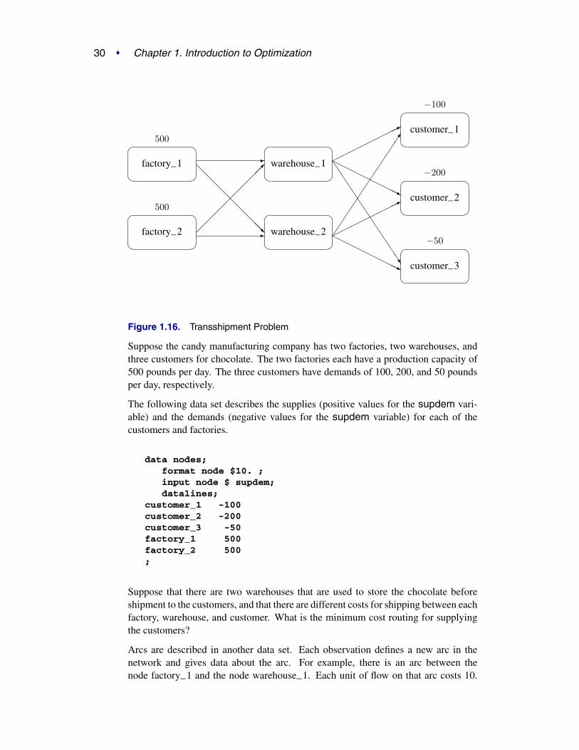
Network flow problems can be described by specifying the nodes in the network andtheir supplies and demands, and the arcs in the network and their costs, capacities,and lower flow bounds. Consider the simple transshipment problem in Figure 1.16 asan illustration.


�

�

�

�factory–2

�

�

�

�factory–1

�

�

�

�warehouse–2

�

�

�

�warehouse–1

�

�

�

�customer–3

�

�

�

�customer–2

�

�

�

�customer–1

�

��

��

��

��

��

��

��

��

��

�

��

��

��

��

��

�

��

��

500

500

−50

−200

−100

Figure 1.16. Transshipment Problem

Suppose the candy manufacturing company has two factories, two warehouses, andthree customers for chocolate. The two factories each have a production capacity of500 pounds per day. The three customers have demands of 100, 200, and 50 poundsper day, respectively.

The following data set describes the supplies (positive values for the supdem vari-able) and the demands (negative values for the supdem variable) for each of thecustomers and factories.

data nodes;format node $10. ;input node $ supdem;datalines;

customer_1 -100customer_2 -200customer_3 -50factory_1 500factory_2 500;

Suppose that there are two warehouses that are used to store the chocolate beforeshipment to the customers, and that there are different costs for shipping between eachfactory, warehouse, and customer. What is the minimum cost routing for supplyingthe customers?

Arcs are described in another data set. Each observation defines a new arc in thenetwork and gives data about the arc. For example, there is an arc between thenode factory–1 and the node warehouse–1. Each unit of flow on that arc costs 10.


Although this example does not include it, lower and upper bounds on the flow acrossthat arc can be listed here.

data network;format from $12. to $12.;input from $ to $ cost ;datalines;

factory_1 warehouse_1 10factory_2 warehouse_1 5factory_1 warehouse_2 7factory_2 warehouse_2 9warehouse_1 customer_1 3warehouse_1 customer_2 4warehouse_1 customer_3 4warehouse_2 customer_1 5warehouse_2 customer_2 5warehouse_2 customer_3 6;

You can use PROC NETFLOW to find the minimum cost routing. This proceduretakes the model as defined in the network and nodes data sets and finds the minimumcost flow.

proc netflow arcout=arc_savarcdata=network nodedata=nodes;

node node; /* node data set information */supdem supdem;tail from; /* arc data set information */head to;cost cost;run;

proc print;var from to cost _capac_ _lo_ _supply_ _demand_

_flow_ _fcost_ _rcost_;sum _fcost_;run;

PROC NETFLOW produces the following messages on the SAS log:

NOTE: Number of nodes= 7 .NOTE: Number of supply nodes= 2 .NOTE: Number of demand nodes= 3 .NOTE: Total supply= 1000 , total demand= 350 .NOTE: Number of arcs= 10 .NOTE: Number of iterations performed (neglecting

any constraints)= 7 .NOTE: Of these, 2 were degenerate.NOTE: Optimum (neglecting any constraints) found.NOTE: Minimal total cost= 3050 .NOTE: The data set WORK.ARC_SAV has 10 observations

and 13 variables.


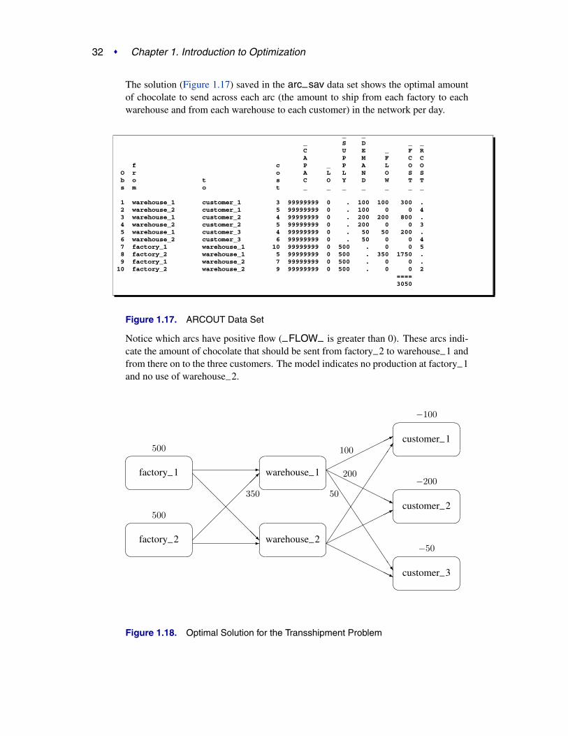
The solution (Figure 1.17) saved in the arc–sav data set shows the optimal amountof chocolate to send across each arc (the amount to ship from each factory to eachwarehouse and from each warehouse to each customer) in the network per day.

_ __ S D _ _C U E _ F RA P M F C C

f c P _ P A L O OO r o A L L N O S Sb o t s C O Y D W T Ts m o t _ _ _ _ _ _ _

1 warehouse_1 customer_1 3 99999999 0 . 100 100 300 .2 warehouse_2 customer_1 5 99999999 0 . 100 0 0 43 warehouse_1 customer_2 4 99999999 0 . 200 200 800 .4 warehouse_2 customer_2 5 99999999 0 . 200 0 0 35 warehouse_1 customer_3 4 99999999 0 . 50 50 200 .6 warehouse_2 customer_3 6 99999999 0 . 50 0 0 47 factory_1 warehouse_1 10 99999999 0 500 . 0 0 58 factory_2 warehouse_1 5 99999999 0 500 . 350 1750 .9 factory_1 warehouse_2 7 99999999 0 500 . 0 0 .10 factory_2 warehouse_2 9 99999999 0 500 . 0 0 2

====3050

Figure 1.17. ARCOUT Data Set

Notice which arcs have positive flow (–FLOW– is greater than 0). These arcs indi-cate the amount of chocolate that should be sent from factory–2 to warehouse–1 andfrom there on to the three customers. The model indicates no production at factory–1and no use of warehouse–2.

�

�

�

�factory–2

�

�

�

�factory–1

�

�

�

�warehouse–2

�

�

�

�warehouse–1

�

�

�

�customer–3

�

�

�

�customer–2

�

�

�

�customer–1

�

��

��

��

��

��

��

��

��

��

�

��

��

��

��

��

�

��

��

500

500

−50

−200

−100

350 50

100

200

Figure 1.18. Optimal Solution for the Transshipment Problem

Model Formats: PROC ASSIGN and PROC TRANS � 33

Model Formats: PROC ASSIGN and PROC TRANS

The transportation and assignment models are described in rectangular data sets.Suppose that instead of sending chocolate from factories to warehouses and then tothe customers, chocolate is sent directly from the factories to the customers.

Finding the minimum cost routing could be done using the NETFLOW procedure.However, since the network represents a transportation problem, the data for the prob-lem can be represented more simply.

data transprt;input source $ supply cust_1 cust_2 cust_3 ;datalines;

demand . 100 200 50factory1 500 10 9 7factory2 500 9 10 8;

This data set shows the source names as the values for the source variable, the supplyat each source node as the values for the supply variable, and the unit shipping costfor source to sink as the values for the sink variables cust–1 to cust–3. Notice thatthe first record contains the demands at each of the sink nodes.

The TRANS procedure finds the minimum cost routing. It solves the problem andsaves the solution in an output data set.

proc transnothrunet data=transprt out=transout;supply supply;id source;

proc print; run;

The optimum solution total (3050) is reported on the SAS log. The entire solution,saved in the output data set transout and shown in Figure 1.19, shows the amount ofchocolate to ship from each factory to each customer per day.

The transout data set contains the variables listed in the transprt data set, and anew variable called –DUAL– . The –DUAL– variable contains the marginal costs ofincreasing the supply at each origin point. The last observation in the transout dataset has the marginal costs of increasing the demand at each destination point. Thesevariables are called dual variables.

Obs source supply cust_1 cust_2 cust_3 _DUAL_

1 _DEMAND_ . 100 200 50 .2 factory1 500 0 200 50 03 factory2 500 100 0 0 04 _DUAL_ . 9 9 7 .

Figure 1.19. TRANSOUT Data Set


Model Building

It is often desirable to keep the data separate from the structure of the model. Thisis useful for large models with numerous identifiable components. The data are bestorganized in rectangular tables that can be easily examined and modified. Then,before the problem is solved, the model is built using the stored data. This process ofmodel building is known as matrix generation. In conjunction with the sparse format,the SAS DATA step provides a good matrix generation language.

For example, consider the candy manufacturing example introduced previously.Suppose that, for the user interface, it is more convenient to organize the data sothat each record describes the information related to each product (namely, the con-tribution to the objective function and the unit amount needed for each process). ADATA step for saving the data might look like this:

data manfg;format product $12.;input product $ object process1 - process4 ;datalines;

chocolate .25 15 0.00 18.75 12toffee .75 40 56.25 0.00 50licorice 1.00 29 30.00 20.00 20jelly_beans .85 10 0.00 30.00 10_RHS_ . 27000 27000 27000 27000;

Notice that there is a special record at the end having product –RHS–. This recordgives the amounts of time available for each of the processes. This information couldhave been stored in another data set. The next example illustrates a model where thedata are stored in separate data sets.

Building the model involves adding the data to the structure. There are as many waysto do this as there are programmers and problems. The following DATA step showsone way to use the candy data to build a sparse format model to solve the productmix problem.

data model;array process object process1-process4;format _type_ $8. _row_ $12. _col_ $12. ;keep _type_ _row_ _col_ _coef_;

set manfg; /* read the manufacturing data */

/* build the object function */

if _n_=1 then do;_type_=’max’; _row_=’object’; _col_=’ ’; _coef_=.;output;

end;

/* build the constraints */

Model Building � 35

do over process;if _i_>1 then do;

_type_=’le’; _row_=’process’||put(_i_-1,1.);end;else _row_=’object’;_col_=product; _coef_=process;output;

end;run;

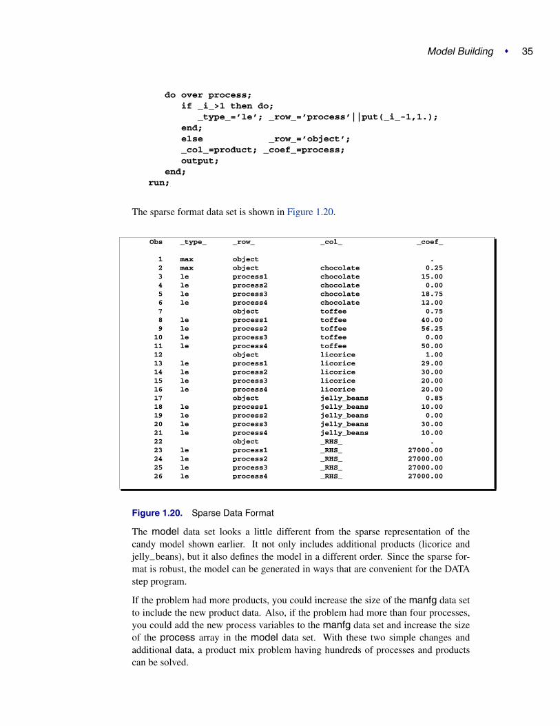
The sparse format data set is shown in Figure 1.20.

Obs _type_ _row_ _col_ _coef_

1 max object .2 max object chocolate 0.253 le process1 chocolate 15.004 le process2 chocolate 0.005 le process3 chocolate 18.756 le process4 chocolate 12.007 object toffee 0.758 le process1 toffee 40.009 le process2 toffee 56.2510 le process3 toffee 0.0011 le process4 toffee 50.0012 object licorice 1.0013 le process1 licorice 29.0014 le process2 licorice 30.0015 le process3 licorice 20.0016 le process4 licorice 20.0017 object jelly_beans 0.8518 le process1 jelly_beans 10.0019 le process2 jelly_beans 0.0020 le process3 jelly_beans 30.0021 le process4 jelly_beans 10.0022 object _RHS_ .23 le process1 _RHS_ 27000.0024 le process2 _RHS_ 27000.0025 le process3 _RHS_ 27000.0026 le process4 _RHS_ 27000.00

Figure 1.20. Sparse Data Format

The model data set looks a little different from the sparse representation of thecandy model shown earlier. It not only includes additional products (licorice andjelly–beans), but it also defines the model in a different order. Since the sparse for-mat is robust, the model can be generated in ways that are convenient for the DATAstep program.

If the problem had more products, you could increase the size of the manfg data setto include the new product data. Also, if the problem had more than four processes,you could add the new process variables to the manfg data set and increase the sizeof the process array in the model data set. With these two simple changes andadditional data, a product mix problem having hundreds of processes and productscan be solved.


Matrix Generation

It is desirable to keep data in separate tables, then automate model building andreporting. This example illustrates a problem that has elements of a product mixproblem and a blending problem. Suppose four kinds of ties are made; all silk, allpolyester, a 50-50 polyester-cotton blend, and a 70-30 cotton-polyester blend.

The data includes cost and supplies of raw material, selling price, minimum con-tract sales, maximum demand of the finished products, and the proportions of rawmaterials that go into each product. The product mix that maximizes profit is to befound.

The data are saved in three SAS data sets. The program that follows demonstrates oneway for these data to be saved. Alternatively, the full-screen editor PROC FSEDITcan be used to store and edit these data.

data material;format descpt $20.;input descpt $ cost supply;datalines;

silk_material .21 25.8polyester_material .6 22.0cotton_material .9 13.6;

data tie;format descpt $20.;input descpt $ price contract demand;datalines;

all_silk 6.70 6.0 7.00all_polyester 3.55 10.0 14.00poly_cotton_blend 4.31 13.0 16.00cotton_poly_blend 4.81 6.0 8.50;

data manfg;format descpt $20.;input descpt $ silk poly cotton;datalines;

all_silk 100 0 0all_polyester 0 100 0poly_cotton_blend 0 50 50cotton_poly_blend 0 30 70;

The following program takes the raw data from the three data sets and builds a linearprogram model in the data set called model. Although it is designed for the three-resource, four-product problem described here, it can be easily extended to includemore resources and products. The model-building DATA step remains essentially thesame; all that changes are the dimensions of loops and arrays. Of course, the datatables must increase to accommodate the new data.

Matrix Generation � 37

data model;array raw_mat {3} $ 20 ;array raw_comp {3} silk poly cotton;length _type_ $ 8 _col_ $ 20 _row_ $ 20 _coef_ 8 ;keep _type_ _col_ _row_ _coef_ ;

/* define the objective, lower, and upper bound rows */

_row_=’profit’; _type_=’max’; output;_row_=’lower’; _type_=’lowerbd’; output;_row_=’upper’; _type_=’upperbd’; output;_type_=’ ’;

/* the object and upper rows for the raw materials */

do i=1 to 3;set material;raw_mat[i]=descpt; _col_=descpt;_row_=’profit’; _coef_=-cost; output;_row_=’upper’; _coef_=supply; output;

end;

/* the object, upper, and lower rows for the products */

do i=1 to 4;set tie;_col_=descpt;_row_=’profit’; _coef_=price; output;_row_=’lower’; _coef_=contract; output;_row_=’upper’; _coef_=demand; output;

end;

/* the coefficient matrix for manufacturing */

_type_=’eq’;do i=1 to 4; /* loop for each raw material */

set manfg;do j=1 to 3; /* loop for each product */

_col_=descpt; /* % of material in product */_row_ = raw_mat[j];_coef_ = raw_comp[j]/100;output;

_col_ = raw_mat[j]; _coef_ = -1;output;

/* the right-hand-side */

if i=1 then do;_col_=’_RHS_’;_coef_=0;output;

end;


end;_type_=’ ’;

end;stop;

run;

The model is solved using PROC LP, which saves the solution in the PRIMALOUTdata set named solution. PROC PRINT displays the solution, shown in Figure 1.21.

proc lp sparsedata primalout=solution;

proc print ;id _var_;var _lbound_--_r_cost_;

run;

_VAR_ _LBOUND_ _VALUE_ _UBOUND_ _PRICE_ _R_COST_

all_polyester 10 11.800 14.0 3.55 0.000all_silk 6 7.000 7.0 6.70 6.490cotton_material 0 13.600 13.6 -0.90 4.170cotton_poly_blend 6 8.500 8.5 4.81 0.196polyester_material 0 22.000 22.0 -0.60 2.950poly_cotton_blend 13 15.300 16.0 4.31 0.000silk_material 0 7.000 25.8 -0.21 0.000PHASE_1_OBJECTIVE 0 0.000 0.0 0.00 0.000profit 0 168.708 1.7977E308 0.00 0.000

Figure 1.21. Solution Data Set

The solution shows that 11.8 units of polyester ties, 7 units of silk ties, 8.5 units ofthe cotton-polyester blend, and 15.3 units of the polyester-cotton blend should beproduced. It also shows the amounts of raw materials that go into this product mix togenerate a total profit of 168.708.

Exploiting Model Structure

Another example helps to illustrate how the model can be simplified by exploitingthe structure in the model when using the NETFLOW procedure.

Recall the chocolate transshipment problem discussed previously. The solution re-quired no production at factory–1 and no storage at warehouse–2. Suppose thissolution, although optimal, is unacceptable. An additional constraint requiring theproduction at the two factories to be balanced is required. Now, the production at thetwo factories can differ by, at most, 100 units. Such a constraint might look like

-100 <= (factory_1_warehouse_1 + factory_1_warehouse_2 -factory_2_warehouse_1 - factory_2_warehouse_2) <= 100

The network and supply and demand information are saved in two data sets.

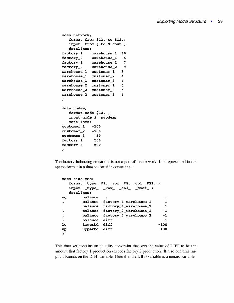
Exploiting Model Structure � 39

data network;format from $12. to $12.;input from $ to $ cost ;datalines;

factory_1 warehouse_1 10factory_2 warehouse_1 5factory_1 warehouse_2 7factory_2 warehouse_2 9warehouse_1 customer_1 3warehouse_1 customer_2 4warehouse_1 customer_3 4warehouse_2 customer_1 5warehouse_2 customer_2 5warehouse_2 customer_3 6;

data nodes;format node $12. ;input node $ supdem;datalines;

customer_1 -100customer_2 -200customer_3 -50factory_1 500factory_2 500;

The factory-balancing constraint is not a part of the network. It is represented in thesparse format in a data set for side constraints.

data side_con;format _type_ $8. _row_ $8. _col_ $21. ;input _type_ _row_ _col_ _coef_ ;datalines;

eq balance . .. balance factory_1_warehouse_1 1. balance factory_1_warehouse_2 1. balance factory_2_warehouse_1 -1. balance factory_2_warehouse_2 -1. balance diff -1lo lowerbd diff -100up upperbd diff 100;

This data set contains an equality constraint that sets the value of DIFF to be theamount that factory 1 production exceeds factory 2 production. It also contains im-plicit bounds on the DIFF variable. Note that the DIFF variable is a nonarc variable.


proc netflowconout=con_savarcdata=network nodedata=nodes condata=side_consparsecondata ;node node;supdem supdem;tail from;head to;cost cost;run;

proc print;var from to _name_ cost _capac_ _lo_ _supply_ _demand_

_flow_ _fcost_ _rcost_;sum _fcost_;run;

The solution is saved in the con–sav data set (Figure 1.22).

_ __ S D _ _

_ C U E _ F RN A P M F C C

f A c P _ P A L O OO r M o A L L N O S Sb o t E s C O Y D W T Ts m o _ t _ _ _ _ _ _ _

1 warehouse_1 customer_1 3 99999999 0 . 100 100 300 .2 warehouse_2 customer_1 5 99999999 0 . 100 0 0 1.03 warehouse_1 customer_2 4 99999999 0 . 200 75 300 .4 warehouse_2 customer_2 5 99999999 0 . 200 125 625 .5 warehouse_1 customer_3 4 99999999 0 . 50 50 200 .6 warehouse_2 customer_3 6 99999999 0 . 50 0 0 1.07 factory_1 warehouse_1 10 99999999 0 500 . 0 0 2.08 factory_2 warehouse_1 5 99999999 0 500 . 225 1125 .9 factory_1 warehouse_2 7 99999999 0 500 . 125 875 .10 factory_2 warehouse_2 9 99999999 0 500 . 0 0 5.011 diff 0 100 -100 . . -100 0 1.5

====3425

Figure 1.22. CON–SAV Data Set

Notice that the solution now has production balanced across the factories; the pro-duction at factory 2 exceeds that at factory 1 by 100 units.

The DATA Step � 41

�

�

�

�factory–2

�

�

�

�factory–1

�

�

�

�warehouse–2

�

�

�

�warehouse–1

�

�

�

�customer–3

�

�

�

�customer–2

�

�

�

�customer–1

�

��

��

��

��

��

��

��

��

��

�

��

��

��

��

��

�

��

��

500

500

−50

−200

−100

225

125

50

100

75

125

Figure 1.23. Constrained Optimum for the Transshipment Problem

Report Writing

The reporting of the solution is also an important aspect of modeling. Since theoptimization procedures save the solution in one or more SAS data sets, report writingcan be written using any of the tools in the SAS language.

The DATA Step

Use of the DATA step and PROC PRINT is the most general way to produce reports.For example, a table showing the revenue generated from the production and a tableof the cost of material can be produced with the following program.

data product(keep= _var_ _value_ _price_ revenue)material(keep=_var_ _value_ _price_ cost);

set solution;if _price_>0 then do;

revenue=_price_*_value_; output product;end;else if _price_<0 then do;

_price_=-_price_;cost = _price_*_value_; output material;

end;run;


/* display the product report */

proc print data=product;id _var_;var _value_ _price_ revenue ;sum revenue;title ’Revenue Generated from Tie Sales’;

run;

/* display the materials report */

proc print data=material;id _var_;var _value_ _price_ cost;sum cost;title ’Cost of Raw Materials’;

run;

This DATA step reads the solution data set saved by PROC LP and segregates therecords based on whether they correspond to materials or products, namely whetherthe contribution to profit is positive or negative. Each of these is then displayed toproduce Figure 1.24.

Revenue Generated from Tie Sales

_VAR_ _VALUE_ _PRICE_ revenue

all_polyester 11.8 3.55 41.890all_silk 7.0 6.70 46.900cotton_poly_blend 8.5 4.81 40.885poly_cotton_blend 15.3 4.31 65.943

=======195.618

Cost of Raw Materials

_VAR_ _VALUE_ _PRICE_ cost

cotton_material 13.6 0.90 12.24polyester_material 22.0 0.60 13.20silk_material 7.0 0.21 1.47

=====26.91

Figure 1.24. Tie Problem: Revenues and Costs

Other Reporting Procedures � 43

Other Reporting Procedures

The GCHART procedure can be a useful tool for displaying the solution to mathe-matical programming models. The con–solv data set that contains the solution to thebalanced transshipment problem can be effectively displayed using PROC GCHART.In Figure 1.25, the amount that is shipped from each factory and warehouse can beseen by submitting the following.

title;proc gchart data=con_sav;

hbar from / sumvar=_flow_;run;

Figure 1.25. Tie Problem: Throughputs

The horizontal bar chart is just one way of displaying the solution to a mathematicalprogram. The solution to the Tie Product Mix problem that was solved using PROCLP can also be illustrated using PROC GCHART. Here, a pie chart shows the relativecontribution of each product to total revenues.

proc gchart data=product;pie _var_ / sumvar=revenue;

title ’Projected Tie Sales Revenue’;run;


Figure 1.26. Tie Problem: Projected Tie Sales Revenue

The TABULATE procedure is another procedure that can help automate solution re-porting. Several examples in Chapter 4, “The LP Procedure,” illustrate its use.

Decision Support Systems

The close relationship between a SAS data set and the representation of the mathe-matical model makes it easy to build decision support systems.

The Full-Screen Interface

The ability to manipulate data using the full-screen tools in the SAS language fur-ther enhances the decision support capabilities. The several data set pieces that arecomponents of a decision support model can be edited using the full-screen editingprocedures FSEDIT and FSPRINT. The screen control language SCL directs dataediting, model building, and solution reporting through its menuing capabilities.

The compatibility of each of these pieces in the SAS System makes construction ofa full-screen decision support system based on mathematical programming an easytask.

References � 45

Communicating with the Optimization Procedures

The optimization procedures communicate with any decision support system throughthe various problem and solution data sets. However, there is a need for the systemto have a more intimate knowledge of the status of the optimization procedures. Thisis achieved through the use of macro variables defined by each of the optimizationprocedures.

References

Rosenbrock, H. H. (1960), “An Automatic Method for Finding the Greatest or LeastValue of a Function,” Computer Journal, 3, 175–184.

chapter 1 introduction to optimization - sas...

Documents