Chapter 1 Mathematical Programming:

an overview Companion slides of

Applied Mathematical Programming by Bradley, Hax, and Magnanti

(Addison-Wesley, 1977) prepared by

José Fernando Oliveira Maria Antónia Carravilla

FORMULATION OF SOME EXAMPLES

Charging a Blast Furnace

An iron foundry has an order to produce 1000 pounds of castings containing at least 0.45 % manganese and between 3.25 % and 5.50 % silicon. As these particular castings are a special order, there are no suitable castings in stock. The castings sell for $0.45 per pound. The foundry has three types of pig iron available in essentially unlimited amounts, with the following properties:

northernwall.blogspot.com

Pig iron is the intermediate product of smelting iron ore with a high-carbon fuel such as coke, usually with limestone as a flux. The term “pig iron” arose from the old method of casting blast furnace iron into moulds arranged in sand beds such that they could be fed from a common runner. The group of moulds resembled a litter of sucking pigs, the ingots being called “pigs” and the runner the “sow”.

Charging a Blast Furnace

Further, the production process is such that pure manganese can also be added directly to the melt. It costs 0.5 cents to melt down a pound of pig iron. Out of what inputs should the foundry produce the castings in order to maximize profits?

“Charging a Blast Furnace” LP Model

Tableau form

Chapter 2

Portfolio Selection

A portfolio manager in charge of a bank portfolio has $10 million to invest. The securities available for purchase, as well as their respective quality ratings, maturities, and yields, are shown in the following table:

Portfolio Selection The bank places the following policy limitations on the portfolio manager’s actions: 1. Government and agency bonds must total at least $4

million. 2. The average quality of the portfolio cannot exceed 1.4 on

the bank’s quality scale. (Note that a low number on this scale means a high-quality bond.)

3. The average years to maturity of the portfolio must not exceed 5 years.

Assuming that the objective of the portfolio manager is to maximize after-tax earnings and that the tax rate is 50 %, what bonds should he purchase? If it became possible to borrow up to $1 million at 5.5 % before taxes, how should his selection be changed?

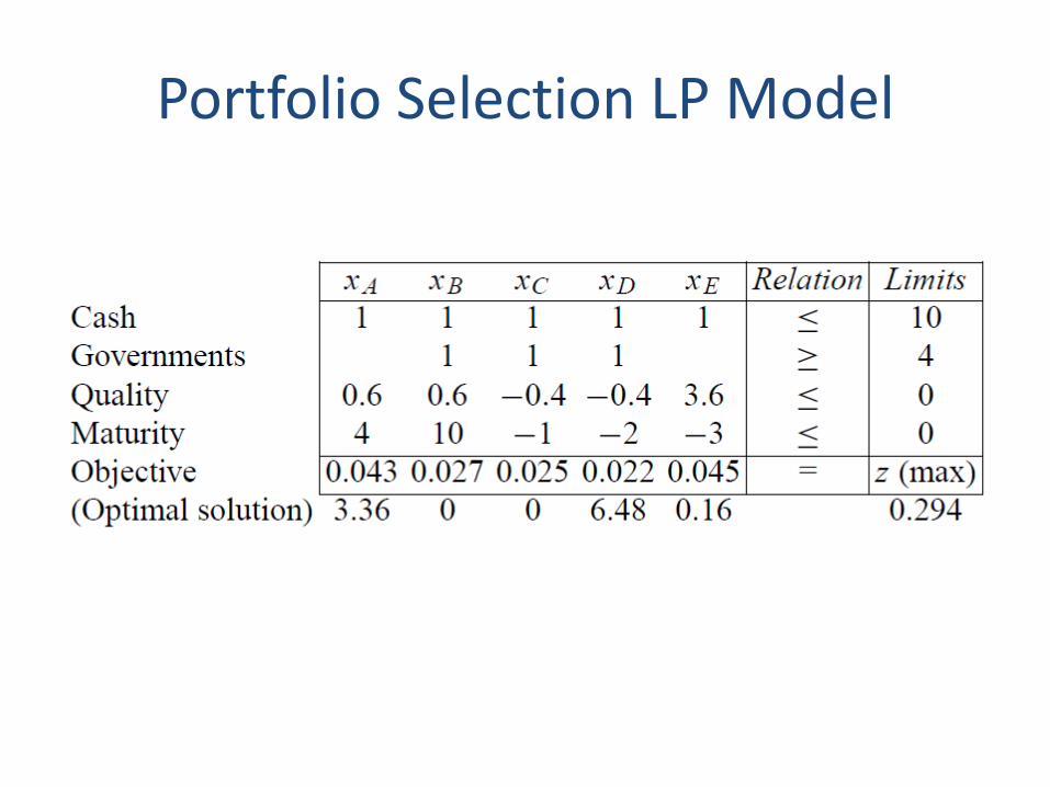
Portfolio Selection LP Model

Portfolio Selection (2nd part)

Now considering the additional possibility of being able to borrow up to $1 million at 5.5 % before taxes. Essentially, we can increase our cash supply above tem million by borrowing at an after-tax rate of 2.75 %:

Production and Assembly

A division of a plastics company manufactures three basic products: sporks, packets, and school packs. A spork is a plastic utensil which purports to be a combination spoon, fork, and knife. The packets consist of a spork, a napkin, and a straw wrapped in cellophane. The school packs are boxes of 100 packets with an additional 10 loose sporks included.

Production and Assembly

Production of 1000 sporks requires 0.8 standard hours of molding machine capacity, 0.2 standard hours of supervisory time, and $2.50 indirect costs. Production of 1000 packets, including 1 spork, 1 napkin, and 1 straw, requires 1.5 standard hours of the packaging-area capacity, 0.5 standard hours of supervisory time, and $4.00 indirect costs. There is an unlimited supply of napkins and straws. Production of 1000 school packs requires 2.5 standard hours of packaging-area capacity, 0.5 standard hours of supervisory time, 10 sporks, 100 packets, and $8.00 indirect costs.

Production and Assembly

Any of the three products may be sold in unlimited quantities at prices of $5.00, $15.00, and $300.00 per thousand, respectively. If there are 200 hours of production time in the coming month, what products, and how much of each, should be manufactured to yield the most profit?

Production and Assembly LP Model 1

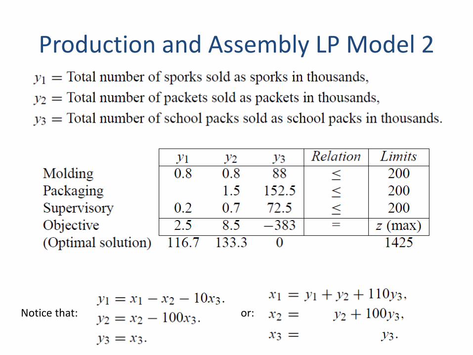
Production and Assembly LP Model 2

Notice that: or:

A GEOMETRIC PREVIEW

The problem Suppose that a custom molder has one injection-molding machine and two different dies to fit the machine. Due to differences in number of cavities and cycle times, with the first die he can produce 100 cases of six-ounce juice glasses in six hours, while with the second die he can produce 100 cases of ten-ounce fancy cocktail glasses in five hours. He prefers to operate only on a schedule of 60 hours of production per week. He stores the week’s production in his own stockroom where he has an effective capacity of 15,000 cubic feet. A case of six-ounce juice glasses requires 10 cubic feet of storage space, while a case of ten-ounce cocktail glasses requires 20 cubic feet due to special packaging.

The problem

The contribution of the six-ounce juice glasses is $5.00 per case; however, the only customer available will not accept more than 800 cases per week. The contribution of the ten-ounce cocktail glasses is $4.50 per case and there is no limit on the amount that can be sold. How many cases of each type of glass should be produced each week in order to maximize the total contribution?

Formulation of the problem

Graphical Representation of the Decision Space

The set of values of the decision variables x1 and x2 that simultaneously satisfy all the constraints indicated by the shaded area are the feasible production possibilities or feasible solutions to the problem.

Finding an optimal solution The optimal solution is at a corner point, or vertex, of the feasible region. This turns out to be a general property of linear programming: if a problem has an optimal solution, there is always a vertex that is optimal.

An optimal solution of a linear program in its simplest form gives the value of the criterion function, the levels of the decision variables, and the amount of slack or surplus in the constraints.

Shadow prices on the constraints

Solving a linear program usually provides more information about an optimal solution than merely the values of the decision variables. Associated with an optimal solution are shadow prices (also referred to as dual variables, marginal values, or pi values) for the constraints. The shadow price on a particular constraint represents the change in the value of the objective function per unit increase in the righthand-side value of that constraint.

Shadow prices on the constraints

For example, suppose that the number of hours of molding-machine capacity was increased from 60 hours to 61 hours. What is the change in the value of the objective function from such an increase?

Shadow prices on the constraints

Shadow prices associated with the non negativity constraints often are called the reduced costs and usually are reported separately from the shadow prices on the other constraints. However, they have the identical interpretation.

Objective and Righthand-Side Ranges

The data for a linear program may not be known with certainty or may be subject to change. When solving linear programs, then, it is natural to ask about the sensitivity of the optimal solution to variations in the data. For example, over what range can a particular objective-function coefficient vary without changing the optimal solution?

Changes in the Coefficients of the Objective Function

We will consider first the question of making one-at-a-time changes in the coefficients of the objective function. Suppose we consider the contribution per one hundred cases of six-ounce juice glasses, and determine the range for that coefficient such that the optimal solution remains unchanged.

Changes in the Coefficients of the Objective Function

We can determine the range on the coefficient of contribution from six-ounce juice glasses, which we denote by c1, by merely equating the respective slopes. Assuming the remaining coefficients and values in the problem remain unchanged, we must have:

Production slope ≤ Objective slope ≤ Storage slope

Changes in the Righthand-Side Values of the Constraints

Throughout our discussion of shadow prices, we assumed that the constraints defining the optimal solution did not change when the values of their righthand sides were varied. Over what range can a particular righthand-side value change without changing the shadow prices associated with that constraint? How much can the production capacity be increased and still give us an increase of $78 4/7 per hour of increase?

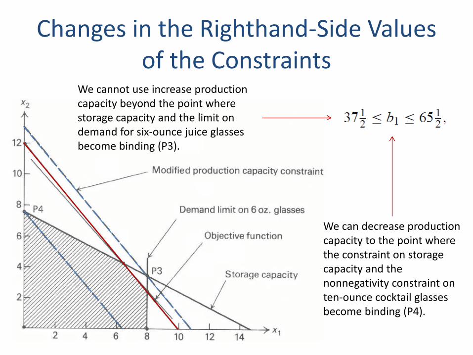
Changes in the Righthand-Side Values of the Constraints

We cannot use increase production capacity beyond the point where storage capacity and the limit on demand for six-ounce juice glasses become binding (P3).

We can decrease production capacity to the point where the constraint on storage capacity and the nonnegativity constraint on ten-ounce cocktail glasses become binding (P4).

Computational considerations

Until now we have described a number of the properties of an optimal solution to a linear program, assuming first that there was such a solution and second that we were able to find it. It could happen that a linear program has no feasible solution. An infeasible linear program might result from a poorly formulated problem, or from a situation where requirements exceed the capacity of the existing available resources.

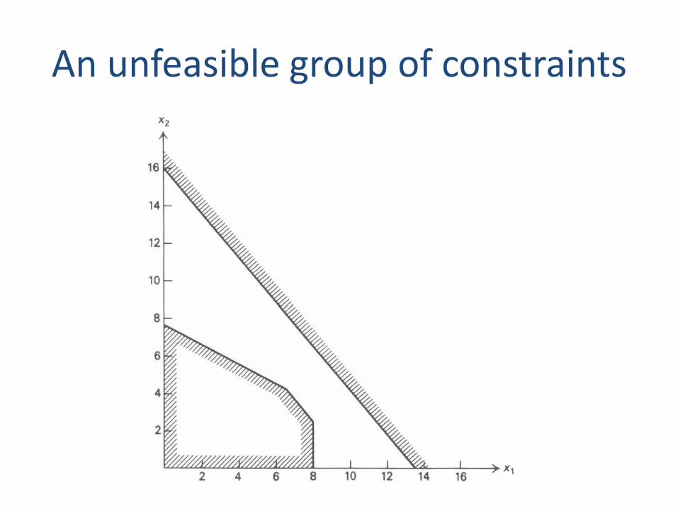
An unfeasible group of constraints

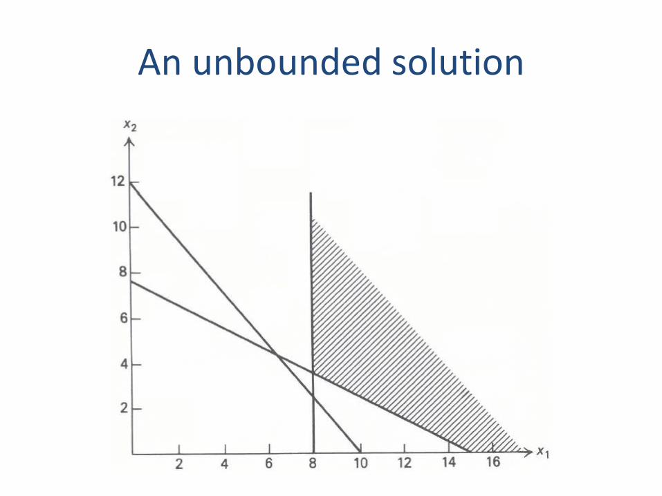
An unbounded solution

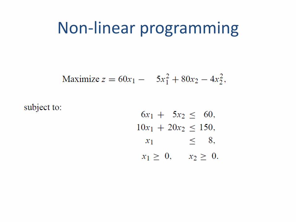
Non-linear programming

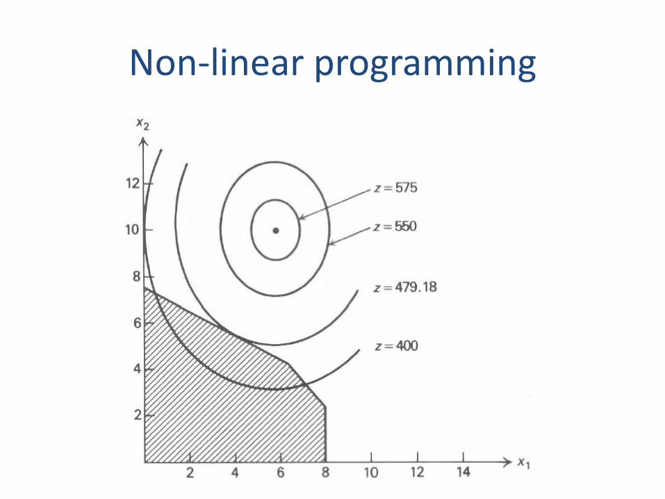
Non-linear programming