chapter 1 overview of the hydrological modeling of small ... · hydrological modeling of small...

CHAPTER 1

Overview of the hydrological modeling of small coastal watersheds on tropical islands

A. FaresCollege of Tropical Agriculture and Human Resources, University of Hawaii-Manoa, Honolulu, HI, USA.

Abstract

Increased population growth especially in coastal areas has resulted in substan-tial land use and land covers changes that in turn have generated concerns about the effects of such activities on their natural resources and especially on the qual-ity and quantity of water resources. Watershed models based upon sound physical theory and well calibrated can provide useful tools for assisting hydrologists and natural-resources managers to choose the best management practices for these sites. This chapter presents an overview of coastal-watershed modeling. It depicts the basic hydrological components of coastal watersheds; it also discusses the different governing equations implemented in the different models to describe the surface and subsurface water fl ow processes simulated by these models. In addition, governing equations for erosion and contaminant transport mechanisms were also presented for physically based and empirical modeling approaches. The chapter discusses the two main approaches (numerical and analytical) of solving the water fl ow and sediment transport governing equations models. Salt water intrusion as a result of natural disasters (Tsunami and hurricanes, e.g. Katrina) was also discussed. This chapter provides an overview of a few coastal-watershed hydrology case studies using different watershed models. By addressing various issues of coastal watershed modeling, this work is intended to assist resource managers, researchers, consultant groups and government agencies to select, use and evaluate different watershed models to be able to adopt sustainable watershed-management practices.

1 Introduction

Rapid growth of global population and changes in economic environment have triggered land-use change that can be linked to changes in climate, biodiversity, and

www.witpress.com, ISSN 1755-8336 (on-line) WIT Transactions on State of the Art in Science and Engineering, Vol 33, © 2008 WIT Press

doi:10.2495/978-1-84564-091-0/01

2 Coastal Watershed Management

water quantity and quality. The impacts of these changes have more pronounced effects on coastal watersheds, especially those of small islands, i.e. Caribbean Islands, Hawaiian Islands, and Pacifi c Islands. A watershed is defi ned as a geo-graphic area of land that drains water to a shared destination such as a river sys-tem or any other water body. The size of a watershed can be small, representing a single tributary within a larger system, or quite large and cover thousands of square kilometers. Small islands are characterized by a large number of small and steep watersheds with highly permeable volcanic rocks and soils. Rainfall is spatially and temporally variable resulting from a combination of both the location within the island and altitude. Tropical rainfall comprises more than two-thirds of the global rainfall [1]. Great variations of rainfall occur within small distances on tropical islands. For example, on the island of Kaua’i, Hawaii annual rainfall increases from 500 mm near Kekaha to over 11,000 mm at Mt. Wai’ale’ale, an average gradient of 0.42 mm/m [2]. This is caused mainly by orographic charac-teristics of rains, which are formed by humid air above oceans carried by trade winds from the sea over the steep and high terrain of the islands. These coastal watersheds contain some of the most productive and diverse natural systems. They comprise complex and highly specialized ecosystems, which extend from the mountains to the adjacent coastal areas that include estuaries, coral reefs, and stream delta, which are vital natural resources for different stakeholders. Intensive management practices in these relatively sensitive environments have generated concerns about the effects of land use/cover changes on the quality and quantity of surface water in adjacent coastal areas and groundwater of the whole system.

Hydrologists are often requested to describe, interpret the behavior of these complex systems. Although some conclusions can be made using best physical and biological science judgments, in many instances human reasoning alone is inadequate to synthesize the collection of factors involved in analyzing complex hydrological problems. Intensive fi eld experiments can be conducted to answer many of these practical management questions; however, such investigations are commonly site specifi c, dependent upon climatological and edaphic conditions, and costly in time and resources.

Hydrological watershed models based upon sound physical theory can provide practical management tools to assist natural-resources managers meet the chal-lenge of description and interpretation. Such management tools combine the sub-tlety of human judgment with the power of personal computers to allow more effective use of available data and account for more complexity. Watershed models have been successfully used to perform complex analyses and to make informed predictions concerning the consequences of proposed actions. They also increased the accuracy of estimates for alternative practices to a level beyond the best human judgment decisions.

1.1 Characteristics of small coastal watersheds on tropical islands

Many unique characteristics of coastal islands result from their isolation, small size and exposure to the marine environment. Most of the tropical islands are the


Hydrological Modeling of Small Coastal Watersheds 3

results of volcanic activities, which make them mountainous in nature, e.g. Hawaii. These islands are continuously exposed to winds, waves, tides, salts, animals, and human activities making them vulnerable to natural and man-made stresses. Generally, the larger the island, the more diverse is its ecosystem, the more varied and numerous are its plants and animals life, and the more tolerant it is to distur-bance. The tropical island climate is strongly moderated by the ocean. Island soils are acidic, infertile, and shallow, with a thin organic layer. Larger islands often contain marshes and bogs. Vegetative cover varies, depending on local conditions, soil type, and past clearing practices. Most of the larger islands are forested and mature softwood stands predominant on their landscapes.

Groundwater is the main source of freshwater on islands, but its depletion and contamination is limiting its use. In tropical islands, groundwater is generated entirely by rain on the island, which percolates into the aquifer. Most of the islands are highly rocky and have impervious soil layers that reduce water infi ltration, causing more surface runoff. Sometimes high groundwater demand under limited source causes saltwater intrusions into the groundwater supply [3]. A methodical understanding of hydrologic cycle components and characteristics of coastal watersheds on tropical islands is needed to select a hydrological model suitable for a particular scenario. This chapter covers the following aims: 1) to describe the main characteristics of hydrological models; 2) to give an overview of available hydrological models applicable to small island coastal watersheds; 3) to review major environmental problems in coastal watersheds; and 4) to present case studies on the application of hydrological models to coastal watersheds.

2 Classifi cation of models

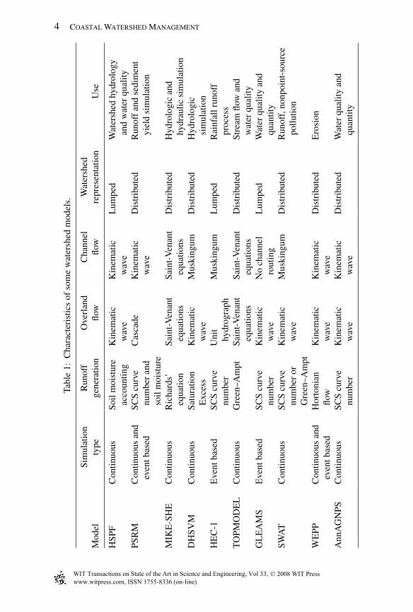
Models are simplifi ed representation of real systems and are often used to predict the response of the modeled system under the infl uence of different management scenarios. Models are classifi ed based on process description (deterministic vs. stochastic), timescale (single event vs. continuous), space scale (distribute vs. lumped), techniques of solution (analytical vs. numerical), and their use (watershed, groundwater) (Table 1).

Physical models are based on the mathematical-physics equations of mass and energy transfer intended to avoid and/or minimize the need for calibration. The phys-ical models are physical representations of a smaller- or larger-scale real system. A physical model is used to simulate some phenomenon on a large-scale by using a small-scale experiment either in a fi eld or a laboratory. Geometric and dynamic scales of physical models are important characteristics. Models can be also classifi ed as linear or nonlinear, deterministic or stochastic, steady state or transient, and lumped or distributed. A linear model is the one in which objective functions are expressed by linear equations. A steady-state model does not account for the element of time, while a transient model is one with an explicit time dimension. A deterministic model is one in which its variables do not vary randomly. Stochastic models have some ran-domness and uncertainty that are described by statistical properties, such as trend, seasonality, mean, variance, skewness, covariance, correlation, and variance function.



Tabl

e 1:

Cha

ract

eris

tics

of s

ome

wat

ersh

ed m

odel

s.

Mod

elSi

mul

atio

n ty

peR

unof

f ge

nera

tion

Ove

rlan

d fl o

wC

hann

el

fl ow

Wat

ersh

ed

repr

esen

tatio

nU

se

HSP

FC

ontin

uous

Soil

moi

stur

e a

ccou

ntin

gK

inem

atic

w

ave

Kin

emat

ic

wav

eL

umpe

dW

ater

shed

hyd

rolo

gy

and

wat

er q

ualit

yPS

RM

Con

tinuo

us a

nd

eve

nt b

ased

SCS

curv

e n

umbe

r an

d s

oil m

oist

ure

Cas

cade

Kin

emat

ic

wav

eD

istr

ibut

edR

unof

f an

d se

dim

ent

yie

ld s

imul

atio

n

MIK

E-S

HE

Con

tinuo

usR

icha

rds’

e

quat

ion

Sain

t-V

enan

t e

quat

ions

Sain

t-V

enan

t e

quat

ions

Dis

trib

uted

Hyd

rolo

gic

and

hyd

raul

ic s

imul

atio

nD

HSV

MC

ontin

uous

Satu

ratio

n E

xces

sK

inem

atic

w

ave

Mus

king

umD

istr

ibut

edH

ydro

logi

c s

imul

atio

n H

EC

-1E

vent

bas

edSC

S cu

rve

num

ber

Uni

t h

ydro

grap

hM

uski

ngum

Lum

ped

Rai

nfal

l run

off

pro

cess

TO

PMO

DE

LC

ontin

uous

Gre

en–A

mpt

Sain

t-V

enan

t e

quat

ions

Sain

t-V

enan

t e

quat

ions

Dis

trib

uted

Stre

am fl

ow a

nd

wat

er q

ualit

yG

LE

AM

SE

vent

bas

edSC

S cu

rve

num

ber

Kin

emat

ic

wav

eN

o ch

anne

l r

outin

gL

umpe

dW

ater

qua

lity

and

qua

ntity

SWA

TC

ontin

uous

SCS

curv

e n

umbe

r or

G

reen

–Am

pt

Kin

emat

ic

wav

eM

uski

ngum

Dis

trib

uted

Run

off,

non

poin

t-so

urce

p

ollu

tion

WE

PPC

ontin

uous

and

e

vent

bas

edH

orto

nian

fl

ow

Kin

emat

ic

wav

eK

inem

atic

w

ave

Dis

trib

uted

Ero

sion

Ann

AG

NPS

Con

tinuo

usSC

S cu

rve

num

ber

Kin

emat

ic

wav

eK

inem

atic

w

ave

Dis

trib

uted

Wat

er q

ualit

y an

d q

uant

ity



Some deterministic models may include stochastic processes to add the dimension of spatial and temporal variability to some of the subprocesses, such as infi ltration. A lumped model does not account for the spatial variability of inputs and outputs parameters, while a distributed model does.

3 Mathematical description of the components of hydrologic cycle

Hydrological models represent one or many components of the hydrological cycle, such as precipitation, infi ltration, evapotranspiration, and runoff. The main com-ponents of the watershed hydrological cycle are briefl y discussed in the following sections.

3.1 Precipitation

Precipitation (rain or snow) is generally one of the most important components of the hydrological cycle. In this text, precipitation and rainfall will be used inter-changeably. Rainfall is characterized by its total amount, duration, intensity and spatial distribution. Under tropical conditions, rainfall is the main form of pre-cipitation and causes most of the water-related disasters. Rainfall is modeled to estimate annual and seasonal water yield, design water-harvesting structures, and predict fl ood peaks, erosion and chemical transport from a given watershed. In most of the tropical islands, the rainfall is spatially and temporally variable, posing complications and challenges for modeling exercises. A stochastic approach has been used to analyze rainfall spatially and temporally. Details on stochastic rainfall model are provided by Loukas et al. [4].

Osborn and Lane [5] identifi ed three major directions in rainfall analysis: (a) determining the optimum sampling in time and space to answer specifi c questions, (b) determining the accuracy of rainfall estimates based on existing sampling sys-tems, and (c) simulating precipitation patterns in varying degree of complexity based on existing sampling system for input to hydrologic models. Loukas and Quick [6] developed an event based watershed response model that uses a linear reservoir-routing technique and simulates the fast runoff. The whole process is infi ltration controlled and they reported good simulation results of the watershed response [6]. Assuming a linear routing, Nash [7] related the storage factor, KF, to the lag time of the watershed as follows:

=1 ,t nKF (1)

where Nash’s n is the number of the linear reservoirs or the shape parameter of the Nash unit hydrograph. The time lag, t1, is defi ned as the time between the centroid of rainfall excess hydrograph and the hydrograph peak. Chuptha and Dooge [8] and Rosso [9] have shown that n is a function of only the geomorphology of the water-shed and KF is a function of the geomorphology and precipitation characteri stic of



the watershed. Yang et al. [10] and Sarino and Serrano [11] reported that KF is the most uncertain parameter of Nash’s model.

3.2 Evapotranspiration

Evapotranspiration is responsible for signifi cant water losses from a watershed. Types of vegetation and land use signifi cantly affect ET. Factors that affect ET include plant type, the plant’s growth stage or level of maturity, rooting depth, per cent soil cover, solar radiation, humidity, temperature, and wind speed. The amount of water transpired depends on the rooting depth of plants because water transpired through leaves is extracted by the roots from the soil in the root zone. Plants with deep-reaching roots can transpire more water than a similar plant with a shallow root system. Solar radiation is the major source of energy for ET and usually contributes from 80 to 100 per cent of the total ET.

Vapor pressure at saturation as a function of air temperature is described by the following equation:

−⎡ ⎤= °⎢ ⎥+⎣ ⎦16.78 116.9

exp for 0 < < 50 C,237.3s

Te T

T (2)

where es is saturation vapor pressure (kPa) and T is air temperature (ºC).Actual vapor pressure of the air (ea) is calculated by the following equation:

= ,

100s

ae RH

e

(3)

where RH is relative humidity.Advancements in the fi eld ET measurement have been signifi cant during the

past three decades. Now, there is a choice of models based on data type and quality, and suitability of fi eld conditions. Watershed models use different ET submodels, i.e. Penman [12], Priestly–Taylor [13], Thornthwaite [14]. Penman [12] mathe-matical model combines the vertical energy budget with horizontal wind effects. ET calculation/measurement has been determined using one of the following: (i) water budget, e.g. Fares and Alva, [15], (ii) mass transfer, e.g. Harbeck, [16], (iii) combination, e.g. Penman, [12], (iv) radiation, e.g. Priestley and Taylor, [13], and (v) temperature based, e.g. Thornthwaite, [14]. Detailed information on many of these methods is available in the literature, e.g. Jensen et al. [17]; and Morton, [18]. Penman model improvements and adaptations were made by many research-ers by including the direct net radiation estimates, improved wind profi le theory and effect of plants [19, 20]. The Penman–Monteith model is probably the most suitable ET model for watershed studies, particularly in tropical islands where high intensity winds have signifi cant effect on ET.

The Penman–Monteith [12] approach includes all parameters that govern energy exchange and the corresponding latent heat fl ux (evapotranspiration)



from uniform expansion of vegetation. It calculates evapotranspiration (mh–1) as follows:

( ) (( ) / ),

(1 ( / ))n a p s a a

s a

R G C e e rET

r r

rl

gΔ − + −

=Δ + +

(4)

where Rn is net radiation (MJ m–2 h–1), G is soil heat fl ux (MJ m–2 h–1), (es – ea) is vapor pressure defi cit of the air (kPa), ra is mean air density at constant pressure (kg m–3), Cp is specifi c heat capacity of the air (MJ m–3 °C–1), Δ is the slope of saturation vapor pressure–temperature relationship times air pressure (kPa °C–1), g is the psychometric constant (kPa °C–1), l is the latent heat of vaporization (MJ m–3), and rs and ra are the surface and aerodynamic resistances (s m–1).

3.3 Infi ltration and subsurface fl ow

Infi ltration is the rate of the downward entry of water into soil; it is one of the most important hydrological processes of the water cycle. Infi ltration is the process that partition water input, e.g. rainfall, irrigation, between the subsurface fl ow and the runoff. It is driven by matric and gravitational forces; thus, factors affecting infi l-tration include soil physical properties, initial water content, rainfall intensity, and soil surface sealing or crust. The infi ltration rate is usually expressed in units of length per unit time. Several efforts have been made to characterize infi ltration for fi eld application including a model based on a storage concept [21] that was later modifi ed by Holtan and Lopez [22]. An approximate model utilizing Darcy’s law was proposed by Green and Ampt [23] that was later modifi ed by several research-ers mainly Bouwer [24], and Chu [25] who applied the Green–Ampt equation for unsteady-state cases. Some of these efforts involved a simple concept that permits the infi ltration rate or cumulative infi ltration rate to be expressed mathematically in terms of time and some soil physical properties. Parameters in such models can be determined from soil water properties based on initial and boundary conditions. Below are a few of the infi ltration models that have been implemented in different watershed models.

Horton [21, 26] developed the following infi ltration model:

,( ) t

p c o cf f f f e b−= + −

(5)

where fp is infi ltration capacity (LT–1), fc is fi nal constant infi ltration rate (LT–1), fo is initial (t = 0) infi ltration rate (LT–1), b is a soil parameter that describes the rate of decrease of infi ltration, and t is time (T). The parameters of Horton’s model, fo, fc, and b are derived based on infi ltration tests.

The Green–Ampt model [23] was based upon a very simple physical model of the soil; it considers that the total saturation is behind the wetting front and the saturated water content is constant but not necessarily total porosity. The original



equation was derived for infi ltration from a ponded surface into a deep homoge-neous soil with uniform water content. Water is assumed to enter the soil as piston fl ow resulting in a sharply defi ned wetting front that separates a zone that has been wetted from totally unwetted zone. Infi ltration capacity (fp) is calculated as follows:

+= ,cw w

p sw

S Lf K

L (6)

where fp is the infi ltration capacity (LT–1), Ks is the saturated hydraulic conduc-tivity (LT–1), Scw is the soil suction at wetting front (L), and Lw is the depth of the wetting front from ground surface.

The depth of the wetting front (Lw) can be related to the cumulative amount of infi ltration, F(L) as follows:

q q= −( ) ,s i wF L (7)

where qs and qi are the saturated and initial soil-water content, respectively.The infi ltration rate f(t) becomes:

q q= + −( ) (1 ( ) / ) for > s cw s i pf t K S F t t

(8a)

=( ) for > ,pf t P t t

(8b)

where tp is the time the water begins to pond at the soil surface.

3.4 Surface fl ow

Surface runoff also known as surface fl ow is that portion of precipitation that, during and immediately following a storm event, ultimately appears as fl owing water in the drainage network of a watershed [27]. Surface fl ow is a major com-ponent of water cycle in coastal area and small-island watersheds where excess water gets much less time to infi ltrate and runs out quickly through streams into the sea. Surface runoff is infl uenced by soil type, rainfall intensity, topography of the watershed, and vegetation type. The theoretical hydrodynamic equations governing the overland fl ow are generally attributed to Barre de St. Venant and were formulated in the late 19th century [27]. The St. Venant equations are based on conservation of mass and conservation of momentum for a control volume. The basic continuity equation is given by:

r

∂=

∂∫∫ ∫∫∫ ,v dA v dVt

(9)

where r is the fl uid density, v is the velocity vector, A is the area vector, t is the time, and V is the volume.

The law of conservation of linear momentum may be expressed as:

r r r∂+ = +

∂∫∫∫ ∫∫ ∫∫∫( ) ,F B dV v v dA v dVt

(10)



where F is the sum of all surface forces on the control volume, and B is the sum of all internal forces per unit mass.

3.4.1 St. Venant equationsThe St. Venant equations are commonly used for prediction and control design for irrigation and drainage channels. This is one of the most commonly used physical-based models for predicting overland fl ow. The St. Venant continuity equation is given by:

∂ ∂ ∂+ =∂ ∂ ∂

0.A v h

v A bx x t

(11)

The dynamic, or momentum, equation is:

∂ ∂ ∂+ = −∂ ∂ ∂

( ),h v v

g v g i jx x t

(12)

where, A is the cross-sectional area of the section, h is the depth of fl ow at the sec-tion, v is the mean velocity at the section, b is the width of the top of the section, x is the position of the section measured from the upstream end, t is the time, g is the acceleration due to gravity, and j is the energy loss/unit length of the channel/ unit weight of fl uid.

The St. Venant equations cannot be solved explicitly except by making some unrealistic assumptions. Therefore, numerical techniques have to be used. The St. Venant equations work under following assumptions:

Flow is one-dimensional• Hydrostatic pressure prevails and vertical accelerations are negligible• Streamline curvature and the bottom slope of the channel are small• Manning’s equation is used to describe resistance effects• The fl uid is incompressible•

3.4.2 Kinematic equationLighthill and Whitham [28] proposed a quasi-steady approach known as the kine-matic wave approximation. The discharge Q after the replacement of the St. Venant equation by a much simpler kinematics wave equation is given by

a= ,mQ y (13)

where, � and m are parameters, and y is the depth of fl ow.The dynamic term in the momentum equation was ignored since it has negligi-

ble affect especially in cases where backwater effects were absent. Woolhiser and Liggett [29] showed that the effect of neglecting dynamic terms in the momentum equation could be assessed by the value defi ned as,

=

2,oS L

kHF

(14)



where, k is the dimensionless parameter is the length of the bed slope, H is the equilibrium fl ow depth at outlet, and F is the equilibrium Froude number for fl ow at the outlet.

3.4.3 SCS methodThe SCS curve number equation is an empirical equation that estimates runoff from small agricultural watersheds by a 24-h rainfall event. The curve number method [27] has been widely used to estimate direct runoff. Runoff (Q) is calcu-lated using the following equation:

−= >

− += ≤

2( )if

( )

0 if ,

aa

a

a

P IQ P I

P I S

Q P I

(15)

where P is the rainfall (in), S is the potential maximum retention after runoff begins (in), and Ia is the initial abstraction (in).

The initial abstraction (Ia) quantifi es the water losses before runoff begins. It is defi ned as a percentage of potential maximum retention (S):

= 0.2 .aI S (16)

The potential maximum retention is a function of curve number:

= −1000

10,SCN

(17)

where CN is the curve number, which ranges from 0 for completely permeable surface to 100 for an impermeable surface but practically ranges between 40 and 98.

The curve number is determined by the hydrologic soil group, cover type, hydrologic condition, and antecedent moisture condition. Although the method is designed for a single storm event, it can be scaled to predict average annual runoff values. For designing fl ood-control structures, the rational method is most com-monly used.

3.4.4 Rational methodSeveral empirical methods of similar form have been developed that require input of rainfall estimates for storms of given frequencies. Possibly the best known and widely used is the simple and aptly named rational formula [30]. The rational equation is an empirical equation that has been used for predicting the peak dis-charge from a small watershed and for design of fl ood-control structures. The peak discharge (ft3 h–1) in rational equation is described as:

= ,q CiA (18)

where C is a runoff coeffi cient, i is rainfall intensity in in h–1 for a given frequency and A is the area of the watershed in acres.



3.5 Subsurface and groundwater fl ow

Darcy [31] found that soil water movement in porous media (q) is directly propor-tional to the hydraulic gradient (i) as follows:

= − ,q Ki (19)

where q is fl ux or volume of water moving through the soil per unit area per unit time (LT–1), K is the hydraulic conductivity (LT–1), which is dependent on the properties of the fl uid and porous medium, i is hydraulic gradient (LL–1) expressed in the x-direction as follows:

= ∂ ∂/ ,i H x (20)

where H is the hydraulic head, which is the sum of the pressure head (h) and eleva-tion head (z).

For saturated soils, the hydraulic conductivity is constant with respect to h; whereas for unsaturated conditions, hydraulic conductivity can vary with time and space if the soil is heterogeneous or anisotropic. In unsaturated conditions, K becomes a function of pressure head (h), then the water fl ux is expressed as follows:

= ∂ ∂( ) / .q K h H x (21)

Water fl ow in variably saturated porous media is described by Richard’s equa-tion that combines the mass balance for an element volume of porous media with Darcy’s law. The 1D form of this equation for fl ow in the vertical direction is as follows:

⎡ ⎤∂ ∂ ∂⎛ ⎞= + ±⎜ ⎟⎢ ⎥⎝ ⎠∂ ∂ ∂⎣ ⎦( ) ( ) 1 ,w

h hC h K h S

t z z (22)

where Cw(h) is the water capacity function which is equal to the inverse slope of h(q), q is water content, and S is the source/sink term. This form of the Richard’s equation has been used to simulate both saturated and unsaturated subsurface fl ow for different initial and boundary conditions.

4 Contaminant transport

Water quality is important for sustainable development in watersheds. Water is the transport agent of energy, nutrient chemicals, and sediments. Increasing amounts of potentially hazardous chemicals released from various agricultural operations have been polluting soil–water ecosystems. Understanding the transport of these chemicals through surface and subsurface water fl ow is essential for the manage-ment of our natural resources to ensure sustainable crop production and minimize pollution of water resources. Farming and ranching have also allowed an excess of nutrients, sediment and chemicals to runoff [32]. Leaching of agrochemicals through the root zone of agricultural crops continues to endanger the long-term



groundwater quality in agricultural areas. Hubbard and Sheredan [33] documented that in many agricultural areas, nitrate-nitrogen (NO3–N) levels in drinking water were signifi cantly higher than the maximum contaminant level of 10 mg L–1 set by the US Environmental Protection Agency.

The fate of a pollutant, in soil, is determined by advection, diffusion and disper-sion processes. In this section different transport processes in saturated (ground-water) and unsaturated (vadose) zones are discussed.

4.1 Surface-water contamination

Surface-water contamination occurs when hazardous substances coming from different sources dissolve or mix with receiving water bodies, e.g. streams, lakes, and oceans. Because of the close relationship between sediments and surface water, contaminated sediments are often considered part of surface-water contamination. Sediments not only contaminate the water but also threat wetlands and streams by depositing pollutants on the bottom of streams, lakes, and oceans. Surface water can be contaminated by hazardous substances either coming from agricultural fi elds or fl owing from an outfall pipe or channel or by mixing with contaminated storm water runoff. Effl uent coming from industrial sources or from some older sewage systems that overfl ow during wet weather to streams can cause substantial amounts of water contamination. Stormwater runoff becomes contaminated when rain water mixes with contaminated soil and either dissolves the contamination held in the soil or carries contaminated soil particles. Surface water can also be contaminated when contaminated groundwater reaches the surface through a rising groundwater table in the rainy season or via a spring.

4.2 Soil erosion

Soil water erosion is the processes of soil detachment, deposition, and transport through a watershed. Erosion is a natural process that can be induced by human activities. There are three main types of soil water erosion: sheet and rill, gully and channel, and mass wasting. Sheet and rill erosion is caused primarily by the action of raindrops and surface-water movement. Raindrops have high energy and initially start the erosion process by splashing and loosening surface soil particles. Gully erosion occurs in well-defi ned channels. Mass wasting occurs when large masses of soil move at once as a result of a landslide, or more slowly over time. Human activities, such as building construction, road construction, timber harvest, grazing, and agriculture activities can accelerate soil-erosion processes.

Soil erosion is a two-stage process. First, sediment is detached, then it is trans-ported. Soil-particle detachment by rainfall is a function of the kinetic energy of the rainfall. After its detachment, suffi cient overland fl ow energy must be available for a soil particle’s transport or it will be deposited. Sediment transport occurs in two associated forms a suspended and a bedload. A suspended load is much more uni-formly distributed throughout the fl ow depth than a bedload. The transport capacity stays mostly in the vicinity of the deposition of suspended sediment due to the



small fall velocities. Bedload is that portion of the load that moves along the bottom of the fl ow by rolling, sliding and saltation. It is generally composed of the larger soil particles, and consequently is highly transport dependent. As such, a decrease in transport capacity causes instantaneous deposition of the excess bedload.

4.3 Modeling soil erosion

Modeling soil erosion has been achieved using physically based models, e.g. rill inter-rill erosion model [34] and empirical models, e.g. USLE [35] and its revised version RUSLE [36].

4.3.1 Empirical erosion modelsThe RUSLE is an empirical model that predicts annual soil water erosion (tons/acre/yr) resulting from sheet and rill erosion in croplands. It is the offi cial tool used for conservation planning in the US. Many other countries have also adapted this model. It is defi ned as follows:

,A = R * K * L * S* C* P (23)

where,A = Annual soil loss (tons acre–1 yr–1) resulting from sheet and rills.R = Rainfall – runoff erosivity factor; it has been mapped for the entire USA.K = Soil erodibility factor; it is a function of the inherent soil properties, including organic matter content, particle size, permeability, etc.L = Slope length factor. This factor accounts for the effects of slope length on the rate of erosion.S = Slope steepness factor; it accounts for the effects of slope angle on erosion rates.C = Cover management factor; it accounts for the infl uence of soil and cover man-agement, such as tillage practices, cropping types, crop rotation, and leaving areas fallow, on soil erosion rates.P = Supporting practices factor; it accounts for the infl uence of conservation prac-tices, e.g. contouring, strip cropping, and terracing.

Despite their wide use in many watershed models, USLE and RUSLE have some theoretical problems, such as interaction among the variables and water fl ow, on which soil loss is closely dependent, is underestimated in the models [37]. It is diffi cult to identify the events that most likely result in large-scale erosion because USLE/RUSLE are not event-responsive equations. They ignore the processes of rainfall-runoff as well as the heterogeneities in input such as vegetation cover and soil types [38]. They do not account for gully erosion, mass movement and sediment deposition [39].

Erosion estimated with these empirical models, e.g. USLE and RUSLE, is often higher than that measured at watershed outlets. The sediment-delivery ratio (SDR) is used to correct for this reduction effect. SDR is defi ned as the fraction of gross erosion that is transported for a given time interval. It is a measure of the sediment transport effi ciency, which accounts for the amount of sediment that is actually



transported from the eroding sources to a measurement point or watershed outlet compared to the total amount of soil that is detached over the same area above that point. In relatively large watersheds, most sediment is deposited within the water-shed and only a fraction of the soil that is eroded from the hillslope reaches the stream network or the watershed outlet.

Physically, SDR stands as a mechanism for compensating for areas of sediment deposition that becomes increasingly important with increasing watershed area. There are many factors that must be addressed when calculating the sediment-delivery ratio in any watershed. Some of the factors that infl uence the SDR include: hydrological inputs (mainly rainfall), landscape properties (e.g. vegetation, topography and soil properties) and their complex interactions at the land surface.

4.3.2 Physically based erosion modelsWater erosion prediction by physically based erosion models, e.g. WEPP [40] uses the physically based rill interrill concept to predict soil erosion [34]. A physically based model computes detachment and transport by raindrop impact, and detach-ment, transport and deposition by fl owing water. It also predicts sheet and rill ero-sion from the top of the hillslope to receiving channel; it also considers sediment deposition. The sediment continuity equation for overland fl ow used is as follows:

( ) ( ),i r

ch cqe e

t x

∂ ∂+ = +

∂ ∂ (24)

where c is total sediment concentration (kg m–3), h is the average, local overland fl ow depth (m), q is discharge per unit width (m2 s–1), x is distance in the direction of fl ow (m), ei is interrill erosion rate per unit area (kg s–1 m–2), and er is net rill erosion or deposition rate per unit area (kg s–1 m–2).

The sediment yield equation assumes constant rainfall [41] for a runoff event and is as follows:

= = + − − −( ) { / ( / )[1 exp( )]/ },s b i r rQ x QC Q B K K B K K x K x

(25)

where Qs is total sediment yield for the entire amount of runoff per unit width of the plane (kg m–1), Q is the total storm runoff volume per unit width (m3 m–1), Cb is mean sediment concentration over the entire hydrograph (kg m–3), Kr and B are rill coeffi cients, Ki is an interrill coeffi cient, K is a slope resistance coeffi cient, x is distance in the direction of fl ow (m), and the other variables are described earlier.

Lane et al. [42] extended this sediment-yield equation for a single plane to irreg-ular slopes approximated by a cascade of planes. From the input data, parameter estimation procedures derived from calibrating WEPP erosion model using rain-fall simulator data were used to compute the depth-discharge coeffi cient, interrill erodibility, rill erodibility, and sediment-transport coeffi cient [43].

4.4 Subsurface-water contamination

Subsurface-water contamination occurs when hazardous substances such as chem-ical fertilizer and pesticides from landfi ll, factory affl uent and agricultural farm



leach to groundwater. Several reviews of solute-transport modeling have been written, such as those by Mercer and Faust [44], Anderson and Woessner [45] and Zheng and Bennett [46]. Freeze and Cherry [47] cover many of the transport equations and offer clear descriptions of many transport mechanisms. Diffusion, dispersion, and advection are the basic processes by which solute moves from one place to another. Diffusion is a molecular-scale process, which causes the spread-ing of the solute due to concentration gradients and random motion. Diffusion causes a solute in water to move from an area of higher concentration to an area of lower concentration. This process continues as long as a concentration gradient exists. The mass of fl uid diffusing is proportional to the concentration gradient, which can be expressed using Fick’s fi rst law.

Dispersion is caused by heterogeneities in the medium that create variation in fl ow velocities and fl ow paths. This variation may occur due to a velocity diffe-rence from one channel to another, or due to variable path lengths. Dispersion is a function of average linear velocity and dispersivity of the medium. Dispersivity in a soil column is on the order of centimeters, while in the fi eld it is on the order of one to one thousand of meters. Mass transport due to dispersion can occur in both longitudinal (parallel to fl ow direction) as well as transverse (perpendicular to fl ow direction) directions. In most cases, transverse dispersivity is much smaller than the longitudinal dispersivity. Hydrodynamic dispersion is the process by which solutes spread out and are diluted compared to simple advection alone. It is defi ned as the sum of the molecular diffusion and mechanical dispersion.

4.5 Solution techniques

4.5.1 Analytical techniquesSeveral analytical models have been developed to solve the water fl ow and solute transport equations for specifi c boundary and initial conditions [48–50]. Analytical solutions are conceptually limited and so does their application to real problems. The geometry of the problem must be regular and simple, e.g. circular, rectan-gular; as such, they are not applicable to complex boundary conditions and are also limited to idealized conditions. Conceptually, analytical solutions are limited by several simplifying assumptions that were used to develop the solution. To overcome these limitations of analytical solution, a numerical approximating tech-nique has been used to solve the transport equations.

4.5.2 Numerical techniquesThese techniques are more fl exible than analytical solutions because they can describe complex systems with proper arrangements of grid cells. In general, these solution techniques break up the study fi eld into small grid cells of differ-ent shapes that best describe the system. These techniques have some limitations. The common numerical methods used to implement mathematical formulation of partial differential equations of fl ow and solute transport are fi nite-difference, fi nite-volume and fi nite-element, method of characteristics, collocation methods, and boundary-element methods as explained by Bedient et al. [51].



The fi nite element and fi nite-difference methods are the most common methods for simulating water fl ow and solute transport. Finite-difference methods are more simple, straightforward and easy to understand. A variety of algorithms were developed to solve fi nite-difference equations. Finite-difference methods represent the simulated system with a grid of square or rectangular shape cells. Partial dif-ferential equations governing water fl ow and solute transport can be approximated by differences and solved by iteration [44]. This approximation leads to errors that can be signifi cant [52]. The fi nite-element method operates by breaking the space in elements of different shapes and sizes that gives more fl exibility to describe irregular simulated systems and variable boundary conditions. The major disad-vantages of the fi nite-element method are its high computing requirement [53] and its diffi cult formulation process.

5 Integrating GIS with watershed models

Geographic information systems play a signifi cant role in facilitating spatial data preparation and analysis because of its ability to store, retrieve, manipulate, analyze, and map geographic data. Using GIS, hydrologists were able to readily produce high-quality maps incorporating model output and geographic entities, further enabling visual support during decision-making processes. Advanced analy-ses and interpretations were possible using several spatial analysis capabilities of the GIS.

Lumped watershed models simplify most of their input parameters and use spatial averaged values for them over the entire simulated watershed. Similarly their out-puts are also spatially averaged. These types of models have been used as great teaching tools; however, they were not embraced as research and management tools to evaluate real management scenarios and nonpoint-source pollution prob-lems. They are unable to determine critical areas of the watershed that are contribu-ting substantially to pollutant loads generated from the watershed of interest. In many nonpoint-source pollution problems, there is a lack of time and resources to conduct intensive fi eld work to identify the spatial contribution of different parts of watersheds to the sediment and pollutant loads leaving a watershed. Thus, use of distributed watershed models is the only viable option that can help manage many of these watersheds with reasonable investment of time and resource.

The use of distributed watershed models has been gaining momentum for the last few decades because of their capabilities in depicting the spatial distribution of water fl ow and erosion processes. However, from the start, their major obstacle was their requirements for large amounts of time and resources needed to assem-ble and manipulate the input and output data sets even for small watersheds. The amount of data increases substantial and consequently so does the time to analyze it as the size of the watershed increases and more heterogeneity is introduced. A logical step in helping watershed hydrologists use distributed watershed models is to interface these models with a practical data management scheme such as geo-graphic information systems (GIS) that would manage, help analyze and display spatially distributed data.



Distributed models create grid/mesh of the simulate watershed domains. These meshes are composed of cells, also know as units. The mesh is generated based on topographic characteristics from the digital elevation model (DEM) data. The water fl ow and sediment transport equations, are solved within each cell at each time step during the duration of simulations. The impact of grid size on the perfor-mance of watershed models is well reported in the literature. A sensitivity analysis that used different grid cell sizes (2, 4, 10, 30 and 90 m) reported signifi cant effects of the grid cell size on the computed topographic parameters and hydrographs [54]. Moore and Thompson [55] found that the slope and topographic index values varied with grid cell size for scales ranging from 20 m to 680 m in three 100 km² study areas in southeastern Australia.

6 Performance of hydrologic model

The performance and behavior evaluation of hydrological models is commonly made through comparison of different effi ciency criteria. To achieve adequate reli-ability of the simulation models, it is important that they are rigorously calibrated and validated before any analysis and/or management scenario analysis are con-ducted. It is highly recommended to do the sensitivity analysis of model param-eters before starting the calibration process. Model calibration and evaluation efforts are performed to achieve a reasonable correspondence between measured fi eld data and the output of the model.

6.1 Sensitivity analysis and model evaluation

Sensitivity analysis is the study of how the variation in the output of a model can be apportioned, qualitatively or quantitatively, to different sources of variation in input. It is the technique of identifying the parameters with little and high impact on the performance of the tested model. Parametric sensitivity is a vital part of most optimization techniques [56]. This modeling tool, if properly used, can pro-vide a better understanding of the correspondence between the model and physical process being modeled. McCuen [56] explained the sensitivity in mathematical form using the Taylor series expansion of the explicit function; thus, from the defi nition, sensitivity S can be given by:

0/ 1 2( , ) ( , , ......., ) / .i i j j i n i

i

FS x F F F x F F F F

F ≠∂ ⎡ ⎤= = + Δ − Δ⎣ ⎦∂

(26)

For parametric and component sensitivity, the factor F0 replaced by an output function (f) and Fi with a parameter under consideration (pi). Thus, the parametric sensitivity, Spi, can be given by:

.pi

i

Sp

∂=

∂f

(27)



Currently, there are several available methods for sensitivity analysis [57, 58]. The new Morris method, in addition to the overall sensitivity, offers estimates of the two factor interaction effects [59]. Several studies have addressed the problem of sensitivity analysis in land-surface schemes using different approaches. Bastidas et al. [60], using the BATS (biosphere-atmosphere transfer scheme) in two different climatic regions of the US showed that a sensitivity analysis performed before the calibration process reduces the number of parameters prompted for calibration. Their fi ndings suggest that the sensitivity analysis is effi cient in reduc-ing the computational time needed in the calibration.

Model evaluation is intimately related to model development. No matter whether models are physically based or conceptually based, they all have some empirical constraints, which could be due to lack of suffi cient observational evidence on some processes and/or limitations set by available computing resources [61]. The model evaluation is an essential process to evaluate the model performance and to assess how well the model represents the real physical system. The purpose of model evaluation is to lead the modeling system toward better results [61]. Model evaluation could be based on anything from accessibility of the model to the real data testing. In modeling terms, the goodness of fi t after calibration between the observed data and simulated data is one way to represent it. There are several ways to express the error between model prediction and real data; i.e. mean absolute error, root mean square error, average relative error and the coeffi cient of effi -ciency given by Nash and Sutcliffe [62].

6.2 Calibration and validation of models

An important part of any modeling exercise is the model calibration. Calibration is a process wherein certain parameters of the model are altered in a systematic fash-ion and the model is repeatedly run until the simulated results match fi eld-observed values within an acceptable level of accuracy. The process of model calibration is quite complex and limited by the model itself, input, and output data. Imperfect knowledge of watershed characteristics, mathematical structures of the hydrologi-cal processes and model limitations can cause error in calibration process. Before starting model calibration, fi eld conditions at the site should be properly charac-terized. Lack of proper site characterization may lead to a wrong representation of the simulated system. There are two primary parts in the model-calibration process [63]. The fi rst is to decide how to judge whether one set of parameters is preferred over another; second is to fi nd the preferred set of parameters. Model calibration can be performed either by trial and error or by automated techniques. Automated calibration can be performed by means of specifying an objective or a set of objective functions [63]. Uncertainty in models and data leads to uncer-tainty in model parameters and model predictions. To avoid these uncertainties, Bevin and Binley [64] proposed generalized likelihood uncertainty estimation (GLUE) that uses prior distributions of parameter sets and a method for updating these estimates as new calibration data becomes available. Automated parameter-estimation techniques for model calibration are accurate and rapid. Validation of



hydrologic models is a process of matching the simulated results with observed values without altering the calibrated parameters. General methodologies related to model calibration and validation has been considerably discussed [65]. How-ever, as noted by Hassanizadeh and Carrera [66] no consensus on methodology exists. Some efforts were made during the past three decades to develop methods for calibration and validation of lumped models, but limited attention has been devoted to distributed models that are relatively more complicated [65]. Refsgaard and Storm [67] emphasized that a rigorous parameterization procedure is crucial in order to avoid methodological problems in the subsequent phases of model calibration and validation.

7 Overview of available hydrologic models

Soil Water Assessment Tool (SWAT): The Soil Water Assessment Tool [68] is a watershed-scale, distributed, conceptual and continuous simulation model, used as a soil and water assessment tool. It can also be used as a fi eld scale model too. There are several versions of SWAT available, and the recent one is SWAT2000 that includes bacteria transport, Green–Ampt infi ltration, the Muskingum routing method, a weather generator, and the SCS curve number for runoff estimation. For potential evapotranspiration calculations, users have options between Penman–Monteith, Priestley–Taylor, and Hargreaves methods. Event-based erosion caused by rainfall and runoff is modeled using a modifi ed universal soil loss equation (MUSLE).

Distributed Hydrology Soil Vegetation Model (DHSVM): This is a distributed, physically based, and continuous simulation watershed and fi eld-scale model. DHSVM was developed by Wigmosta et al. [69] at the University of Washington, Seattle. This model accounts for topographic effects on soil moisture, groundwater, and surface-water relocation in a complex topography. It includes canopy inter-ception, evaporation, transpiration, and snow accumulation and melt, as well as runoff generation via the saturation excess mechanisms. Canopy evapotranspira-tion is represented via a two-layer Penman–Monteith formulation that incorporates local net solar radiation, surface meteorology, soil characteristics and moisture status, and a species-dependent leaf-area index and stomatal resistance. Snow accumulation and ablation are modeled using an energy-balance approach that includes the effects of local topography and vegetation cover. Saturated subsurface fl ow is modeled using a quasi-three-dimensional routing scheme.

System Hydrologique Européen (MIKE SHE): The original MIKE SHE [70] model was developed and became operational in 1982, under the name Système Hydrologique Européen (SHE). The model was sponsored and developed by three European organizations: the Danish Hydraulic Institute (DHI), the British Institute of Hydrology, and the French consulting company SOGREAH. MIKE SHE is an integrated, physically based, distributed model that simulates hydrological and water-quality processes on a basin scale. This model is able to simulate both sur-face and groundwater with precision equal to that of models focused separately on either surface water or groundwater. The MIKE SHE modeling system simulates



most major hydrological processes of water movement, including canopy and land-surface interception after precipitation, snowmelt, evapotranspiration, over-land fl ow, channel fl ow, unsaturated subsurface fl ow, and saturated groundwater fl ow. It also simulates major water-quality components. A grid network represents spatial distributions of the model parameters, inputs, and results with vertical layers for each grid. MIKE SHE uses the Kristensen and Jensen [71] method for calculating actual evapotranspiration. It includes Muskingum and Muskingum–Cunge methods for simplifi ed channel routing.

Annualized Agricultural Nonpoint-Source Model (AnnAGNPS): Annualized Agricultural Nonpoint Source designed by the US Department of Agriculture (USDA ARS and NRCS), is a continuous distributed simulation model widely used for watershed assessment. It expands the capabilities of its predecessor AGNPS [72] which is a single-event model. Runoff is calculated using the SCS curve number equation [73], but is modifi ed if a shallow frozen surface soil layer exists. Curve numbers are modifi ed daily based upon tillage operations, soil mois-ture, and crop stage. Actual evapotranspiration is a function of potential evapo-transpiration calculated using the Penman–Monteith equation [12] and soil-water content. Soil water erosion is estimated using RUSLE [36] that was modifi ed to be implemented at the watershed scale in AnnAGNPS [74]. AnnAGNPS uses a GIS interface for processing input and output data. However, selecting the proper grid size was identifi ed as a major factor infl uencing sediment yield calculations [75]. The border conditions before a rainfall-runoff event are calculated by the model rather than by individual user input. Additionally, long-term simulations are pos-sible using AnnAGNPS as compared to event-based AGNPS model.

Nonpoint-Source Pollution and Erosion Comparison Tool (N-SPECT): The coastal services center of the National Oceanic and Atmospheric Administration (NOAA) developed the Nonpoint-Source Pollution and Erosion Comparison Tool (N-SPECT) to examine the relationships between land cover, soil characteristics, topography, and precipitation in order to assess spatial and temporal patterns of surface-water runoff, nonpoint-source pollution, and erosion. N-SPECT was developed as a decision-support tool for coastal watersheds. N-SPECT uses the SCS curve number method for runoff estimates and generates a curve number grid based on the combination of land cover and hydrological soil group at each cell within a given study area. Soil erosion is calculated either using RUSLE or MUSLE equations when the model is used to simulate annual or single event, respectively.

Physically Based Runoff Prediction Model (TOPMODEL): This is a physically based distributed, continuous simulation watershed model. TOPMODEL was developed by Beven and Kirkby [76], it predicts watershed discharge and a spatial soil-water saturation pattern based on precipitation and evapotranspiration time series and topographic information. TOPMODEL is a set of conceptual tools that can be used to reproduce the hydrological behavior of watersheds in a distributed or semidistributed way. The Penman–Monteith method is implemented in the model to estimate ET. Runoff is computed according to the infi ltration excess mechanism, thus, TOPMODEL uses the exponential Green–Ampt equation of Beven [77]. Detailed background information of the model and some of its applications can be



found in Beven [78]. TOPMODEL assumes that whole basin is homogeneous, which could be unrealistic and applicable for only smaller basins. The model is very sensitive to parameters like soil hydraulic conductivity decay, the soil trans-missivity at saturation, the root zone storage capacity and the channel routing velo-city in larger watersheds [79]. The calibrated values of parameters are also related to the grid size used in the digital terrain analysis [80–82]. The time step and the grid size have also been shown to infl uence TOPMODEL simulations [83].

Hydrological Simulation Program – FORTRAN (HSPF): The Hydrological Simulation Program – FORTRAN (HSPF) was developed by the EPA-Athens laboratory [84]. HSPF is a comprehensive, conceptual, continuous watershed simulation model that simulates the water quantity and quality processes that occur in a watershed, including sediment transport and movement of contaminants. It is an analytical tool that has application in planning, design, and operation of water-resources systems. The model enables the use of probabilistic analysis in the fi elds of hydrology and water-quality management through its continuous simulation capability. This model is classifi ed as a lumped model, but it can reproduce spatial variability by dividing the basin in hydrologically homogeneous land segments and it can simulate runoff for each subbasin independently, using different meteo-rological input data and watershed parameters. Runoff fl ow rate, sediment loads, nutrients, pesticides, toxic chemicals, and other water-quality constituent concen-trations can be predicted. The model can simulate continuous, dynamic, or steady-state behavior of both hydrologic/hydraulic and water-quality processes in a watershed. HSPF also may be applied to urban watersheds through its impervious-land module. A large number of parameter requirements increases the problem associated with parameter selectivity and physical meaningfulness of model parameters. The model relies heavily on calibration against fi eld data for parame-terization [85]. HSPF does not explicitly model agricultural management practices and their effects on runoff or water quality.

Water-Erosion Prediction Project (WEPP) Model: The WEPP erosion model, developed by USDA-ARS is a continuous simulation computer program that pre-dicts soil loss and sediment deposition from overland fl ow on hill slopes, soil loss and sediment deposition from concentrated fl ow in small channels, and sediment deposition in impoundments. In addition to the erosion components, it also includes a climate component that uses a stochastic generator to provide daily weather information, a hydrology component that is based on a modifi ed Green–Ampt infi ltration equation and solutions of the kinematic wave equations, a daily water-balance component, a plant growth and residue decomposition component based on the erosion productivity impact calculator (EPIC) model, and an irrigation component. The WEPP model computes spatial and temporal distributions of soil loss and deposition, and provides explicit estimates of when and where in a water-shed or on a hill slope erosion might occur so that appropriate conservation mea-sures can be selected to best control soil loss and sediment yield. Theoretically, it can exactly predict how rainfall will interact with the soil on a site during a particular rainstorm or during the course of an entire year [86]. The model uses the soil–water-balance component based on the corresponding component of the



simulator for water resources in rural basins (SWRRB) model [87]. The infi ltration component of the hill slope model is based on the Green and Ampt equation as modifi ed by Mein and Larson [88], with the ponding-time calculation for an unsteady rainfall [25]. The water-balance and percolation components of the hill-slope model are based on the water-balance component of the SWRRB [87], with some modifi cations for improving estimation of percolation and soil evaporation parameters. WEPP considers only Hortonian fl ow or fl ow that occurs when the rainfall rate exceeds the infi ltration rate. The model uses two methods of comput-ing the peak discharge: a semianalytical solution of the kinematic-wave model and an approximation of the kinematic-wave model. The fi rst method is used when WEPP is run in single-event mode, while the second is used when WEPP is run in continuous simulation mode [89, 90]. WEPP requires large number of data sets that may limit model use in watersheds where relatively less data is available. Many of the model parameters need to be calibrated to avoid problems with model identifi ablity and the physical interpretability of model parameter [38]. The WEPP model does not include gully erosion and the rill-interrill concept of erosion that may limit its application for all types of soil and fi eld conditions [38]. WEPP does not model nitrate or phosphorus losses from agricultural landscapes.

CREAMS/GLEAMS: Chemicals, runoff, and erosion from agricultural man-agement systems (CREAMS) model [91] was developed by the US Department of Agriculture-Agricultural Research Service to aid in the assessment of agricultural best management practices for pollution control. CREAMS is commonly used for evaluation of agricultural best management practices (BMPs) for pollution control. Daily erosion, sediment yield, and associated nutrient and pollutant loads are estimated at the boundary of the agricultural area. Runoff estimates are based on the SCS curve number method. CREAMS calculates runoff volume, peak fl ow, infi ltration, evapotranspiration, soil-water content, and percolation on a daily basis. Daily erosion and sediment yield are also estimated and average concentra-tions of sediment associated and solute chemicals are calculated for the runoff, sediment, and percolating water [91]. By incorporating a component for vertical fl ux of pesticides in the root zone, the groundwater loading effects of agricultural management systems (GLEAMS) model [92] was established. GLEAMS is parti-tioned into three components, namely hydrology, erosion/sediment yield, and pes-ticides. Surface runoff is estimated using the SCS Curve Number Method [93]. Soils are divided into multiple layers of varying thickness for water and pesticide routing [92]. Both CREAMS and GLEAMS are maintained by the USDA Agricul-tural Research Service. The major limitation of the model is that it is a lumped model, it assumes the whole watershed is uniform in soil topography and land use, a highly unrealistic assumption.

8 Specifi c environmental problems in coastal watersheds

Saltwater intrusion is a natural process infl uenced by humans; it occurs in almost all coastal aquifers. Saltwater intrusion is the movement of salt water into fresh-water resources, such as a groundwater aquifer or a freshwater marsh. This intrusion



may occur as the result of a natural process like a storm surge from a hurricane. For freshwater, more often it results from human activities such as construction of navigation channels or oil fi eld canals. Climate change has led to a rise in sea level with loss of coastal wetlands and increased saltwater intrusion [94]. The December, 2005 tsunami in the Indian Ocean and Hurricane Katrina in New Orleans and southern Louisiana (August, 2005) resulted in salt-water intrusion into surface and subsurface freshwater sources. Salt water intrusion into water bodies such as rivers, wells, inland lakes, and groundwater aquifers has occurred in many of the affected countries. A post-tsunami study conducted by the Indian Agricultural Research Institute [95] showed that in deep brown coastal soil zones, the quality of shallow groundwater has deteriorated. The electrical conductivity of shallow groundwater (25 m below ground level) changed from the pretsunami value of 0.5 dS m–1 to the post tsunami value of 4.8 dS m–1. An estimated 62,000 groundwater wells were contaminated by seawater in Sri Lanka alone. However, in the Maldives islands saltwater intrusion from the tsunami has rendered many of the reservoirs useless. The extent of damage caused by these natural disasters to groundwater resources is still unknown and needs to be assessed.

The coastal areas of the world accommodate high populations and overexploitation of the groundwater has become a common issue along the coast where good-quality groundwater is available. Consequently, many coastal regions in the world experience extensive saltwater intrusion in aquifers resulting in severe deterioration of the quality of groundwater resources. The extent of this saltwater intrusion depends on climatic conditions, aquifer characteristics and groundwater use. In Australia, serious prob-lems of saltwater intrusion exist in the coastal plain of Queensland [96–98]. Many coastal areas in the United States have experienced sea-water intrusion due to both increased groundwater withdrawal and increased urbanization [99].

Saltwater-intrusion problems in coastal aquifers are not new and different research-ers have used different numerical and physical techniques to simulate the problem. The initial model was developed independently by Ghyben in 1888 and by Herzberg in 1901. This simple model is known as the Ghyben–Herzberg model and is based on the hydrostatic balance between fresh and saline water in a U-shaped tube. They showed that the saltwater occurs at a depth h below sea level represented by:

rr r

=−

,sf

s f

h h

(28)

where, rf and rs are, respectively, the density of fresh and saline water, and hf is the elevation of fresh water level above mean sea level. More detailed information on the subject is covered in this book by Dogan and Fares (Chapter 8)

9 Applications of hydrologic models to coastalwatersheds: case studies

Earlier in the chapter, we talked about different types of watershed modeling approaches of rainfall runoff and sediment transport. This section focuses on



overviewing some of the watershed hydrology studies that use some of the water-shed models described in previous sections of the chapter.

A study of nonpoint-source modeling was published by Corbett et al. [100] on a forested and urban watershed in South Carolina coast. The two selected watersheds were 27 km apart and were adjacent to high-salinity salt marshes. Storm-water run-off volumes, fl ow rates, and sediment loads from both watersheds were compared based on 10 rainfall events using the agricultural nonpoint-source (AGNPS) model. Their results show that although AGNPS was intended for agricultural watersheds, it can also simulate forested and urban watershed reasonably well. Simulation results reported signifi cantly higher runoff volume (14.5%) and sediment loads from the urban watershed than from the forested watershed. In the AGNPS model, runoff volumes were governed by the total impervious area and ignoring the spatial charac-teristics of watershed, i.e. size, shape, location, and contiguity. Adding simulated impervious surface area increased runoff volumes linearly and peak fl ow rates exponentially. Flow rates and sediment loads were controlled by impervious surface spatial characteristics. The authors reported maximum sediment loads from the urban watershed when disconnected patches of impervious surface covered 35% of the watershed. Maximum differences between the forested and urban watersheds occurred at low rainfall depths [100]. They recommended the incorporation of groundwater dynamics, the spatial and temporal variability of rainfall, and accumu-lation and wash-off of specifi c pollutants [100].

Vieux and Needham [101] studied the sensitivity of AGNPS to variations of grid-cell sizes in an agricultural and forested watershed near Morris, Minnesota. By varying the grid cells between one hectare and 16 hectares, simulated fl ow path lengths were seen to decrease with increasing grid-cell size. A corresponding vari-ability in AGNPS sediment yield was also observed due to change in fl ow path length. It was observed that the sediment-delivery ratio using the one-hectare grid cells, was 71% greater than the 16-hectare grid-cells. This research showed that cell-size selection for a discrete watershed analysis should be based on the spatial variability of parameters in the watershed.

The Texas Natural Resource Conservation Commission (TNRCC) published a study of water quality in the Nueces Coastal Basins in 1994. TNRCC used GIS techniques for the establishment of a nonpoint-source pollution-potential index (NSPPI) in an effort to identify areas with high potential risk of nonpoint-source loadings. Components of the NSPPI are based on the RUSLE equation [36]. In addition to the elements from the RUSLE, the NSPPI also includes nonsediment-related hazardous pollutants, such as pesticides or heavy metals. For each of the input parameters to the RUSLE equation and independent related hazardous pol-lutant factors in the pollution-potential index, a separate GIS layer, was created with component values assigned to the reclassifi ed polygons from the original source map. Through application of this index to the study areas of the San Antonio–Nueces and Nueces–Rio-Grande coastal basins, Texas, the TNRCC concluded that the region generally had a moderate potential for nonpoint pollutant sources, but that areas of higher potential are the agricultural land in regions of maximum slope and erodible soils [102].



Baird et al. [101] compared the effectiveness of SWAT [67] and HSPF [84] to assess nonpoint-source pollution. They found that average annual predicted stream-fl ow was approximately 10% less than the average observed streamfl ow over the period between 1987 and 1992. Predicted streamfl ow values for each year between 1986 and 1993 showed errors in excess of 68%, when compared with observed annual streamfl ow values [103]. However, they also reported that the average annual predicted streamfl ow calculated by HSPF was within 0.4% of the average observed value over the period from 1987 to 1992.

Nutrient and sediment loadings were predicted using HSPF by applying expected mean concentration values to land uses in the Oso Creek watershed, Austin, Texas. They presented sets of land-use-based loads for each month in the eight-year mod-eling period. Summation of the land-use-based loads resulted in a total load of pollutant from the watershed. Variability of the loadings from year to year natu-rally corresponded to the observed variability of stream fl ows from year to year [104]. Overall, the HSPF model was seen to be more robust and to provide more accurate results than the SWAT model. Cuo et al. [104] used the DHVSM model to simulate the soil moisture, net radiation and stream fl ow in a tropical mountain-ous watershed in Pang Khum, Chang Mai, Thailand. They reported that the model performed reasonably well despite being applied in a region and at a scale that contrasted strongly with those in which it was developed. DHSVM computes the channel discharge for each channel segment using a linear reservoir routing scheme. It incorporates lateral infl ow via both overland fl ow and intercepted sub-surface fl ow [69, 105]. Doten et al. [106] evaluated the road-removal scenario and a basin-wide fi re scenario in a mountainous forested watershed. Their study under forest fi re, showed an increase in all erosion components due to decreases in root cohesion and increases in surface runoff and thus transport capacity. Also, road erosion rate decreased with decreasing road density. Cuo et al. [104] reported that road signifi cantly alters the runoff and they attributed the effect to Horton Over-land Flow (HOF) generated on the road surface. Ziegler et al. [107] reported that the use of a HOF-based model to simulate runoff and sediment transport on unpaved roads provides not only lower-bound estimates of these processes, but also realistic approximations for typical events.

A numerical modeling exercise was carried out [108] using a modifi ed version of the SHARP model to study the groundwater withdrawal in Lihue basin, Kauai, Hawaii. Izuka and Gingerich [109] studied the effects of groundwater withdrawals proposed for Hanamaulu and Puhi, Kauai, Hawaii. The Lihue Basin is a large semicircular depression in southeastern Kauai, the fourth-largest island (553 miles2) in the tropical, north-Pacifi c archipelago of Hawaii. The simulations were carried out in both steady and transient states at different pumping rates. Simulated groundwater withdrawals in the model were based on water-use data obtained in 1993 from the Hawaii State Commission on Water Resources Management.

Numerical simulations indicate that groundwater withdrawals from the Hanamaulu and Puhi areas of the southern Lihue Basin will result in depression of water levels and reductions in stream base fl ows in and near proposed new water-supply wells. Except for areas such as Puhi and Kilohana, which have unique



hydraulic characteristics that are of limited extent, the freshwater lens in most inland areas of the southern Lihue Basin is thick and hydraulic conductivities are low. Effects of the projected withdrawals on streams depend on the withdrawal rate and proximity of the pumped wells to streams. However, shifting ground-water withdrawals away from streams with small base fl ow and toward streams with large base fl ow can reduce the relative effect on individ ual streams.

Mair et al. [110] evaluated streamfl ow, rainfall, and ground-water pumping data for the upper part of the Makaha valley coastal watershed on the island of Oahu, Hawaii to identify corresponding trends and relationships. They found that stream-fl ow declined over the 46-year period of record during the ground-water pumping period. Mean and annual streamfl ow declined by 42% (135 mm) and 56% (175 mm), respectively, and the mean number of dry stream days per year increased from 8 to 125. Rainfall across the study area appeared to have also declined though it was not clear whether the reduction in rainfall was responsible for all or part of the observed streamfl ow decline. Mean annual rainfall at one location in their study area declined by 14% (179 mm) and increased by 2% (48 mm) at the watershed head water.

Fares [111] evaluated the performance of AnnAGNPS watershed model, in sim-ulating runoff and soil erosion in a 50-km2 watershed located on the Island of Kauai, Hawaii. The model was calibrated and validated using 2 years of observed stream fl ow and sediment load data. Alternative scenarios of spatial rainfall distri-bution and canopy interception were evaluated. They reported that initially, the model produced high CN values, which resulted in increased simulated runoff. To overcome this problem the initial CN values were reduced to their lower limit values for the corresponding land-cover types. Simulations showed that in order to account for the canopy-interception effect, a site-specifi c canopy-interception model was preferable over the algorithm provided in AnnAGNPS. Accurate repre-sentation of the spatial distribution of precipitation is critical for accurate model performance. It was demonstrated that even with a limited number of climate stations within the watershed, an adequate representation of spatial rainfall distri-bution can be achieved using an accurate annual precipitation map. Monthly runoff volumes predicted by AnnAGNPS compared well with the measured data (R2 = 0.90), however, up to 60% difference between the actual and simulated run-off were observed during the driest months (May and July). Prediction of daily runoff was less accurate (R2 = 0.55).

During sensitivity analysis it was found that sediment yield from the watershed was closely related to: vegetation root mass, average canopy fall height, soil erod-ibility, percentage of ground residue cover, and canopy cover ratio. The latter two parameters had the greatest infl uence on sediment yield. The entire watershed was covered by dense vegetation, which protects the soil from direct rainfall impact. Under these conditions high sediment yield was observed on areas with low clay content and on steep slopes. The RUSLE erosion factor K, which is directly related to soil properties, was the single most important parameter, which infl uenced the spatial variability of sediment losses. Predicted and observed sediment yields on a daily basis were moderately correlated (R2 = 0.5). For the events of small magnitude,



the model generally overestimated sediment yield, while the opposite was true for larger events. Total monthly sediment yield varied within 50% of the observed val-ues, except for May 2004. It was found that approximately one third of the watershed area had low sediment yield (0–1 t ha–1 y–1), and presented limited erosion threat. However, fi ve per cent of the area had sediment yields in excess of 5 t ha–1 y–1. Fifty one per cent of the total area of the watershed contributed with less than 10% of total sediment generated; however, 49% of watershed generated over 90% of the total sediment. The results are based on the use of original NRCS soil classifi cation and USGS land-cover maps with baseline curve numbers.

The model was recalibrated due to the availability of an updated NRCS soil clas-sifi cation and a higher resolution and species-specifi c land-cover map developed by USGS [111, 112]. Predicted runoff and sediment load using the new parameters were more accurate compared to those estimated with the original soil classifi cation and Landsat land-cover map. For 2003, runoff and sediment were overpredicted by 99% of the measured values. The recalibrated input parameters were used to predict runoff and sediment for 2004 as well. The USGS land-cover map with the updated soil classifi cation produced slight overestimates of runoff and sediment load.

In Hanalei, Feral pigs are one of the major causes of pollution. The soil distur-bance due to their activities in the watershed results in increased sedimentation in the bay. The implementation of feral pig damage estimates resulted in a substantial increase of sedimentation due to the high sensitivity of the model to the surface residue cover parameter. With nearly 90% of the study area affected by feral pig activity, as a result, the predicted sedimentation was almost 2.5 times larger than that without pig damage. This substantial increase in sedimentation was expected due to sensitivity of the model to the surface residue cover parameter.

10 Summary

Considerable concern has arisen over potential ecological and environmental impacts of nonpoint-source pollution originating from different parts of coastal watersheds as a result of different management practices and land-use changes. A number of experimental investigations have been reported in the literature for acquiring information essential to optimum watershed management, conservation, and regulatory decision. Impacts of different management practices may range from a few days to several years. Unfortunately, fi eld investigations are typically site and weather specifi c. Thus, total reliance upon results from fi eld experiments requires a very large resource base acquired over a long time span.

Watershed models offer practical tools optimizing two fi nite management assets, time and money. Modeling endeavors may be used to lessen the number of fi eld experiments required, and underscore important parameters and variables that most infl uence this system. A combination of carefully planned fi eld investigations and physically based distributed watershed models offers an effective means to make informed analyses and/or predictions concerning sensitive coastal watersheds.

The hydrology of most coastal watersheds is very similar; however, the hydrology of small islands watersheds has many unique features due to the strong dominance



of the surrounding ocean, the continuous effect of prevalent winds, steep topography and their relatively small size. Although these islands have substantial amounts of surface water, groundwater is the main source of their freshwater and as such its contamination is limiting its use. Most of these islands are highly rocky and have impervious soil layers that reduce water infi ltration, causing more surface runoff.

After an overview of the some of the major criteria on classifi cation of watershed models the chapter gives an overview of some of the watershed models currently used and featured in the literature. Because this overview information was tabu-lated, it allows for a practical comparison between these different models using the following criteria: simulation type, runoff generation, overland fl ow, channel fl ow, watershed representation, and their use. This information will be useful for the users to help them select the appropriate model based on their modeling needs.

Many of the mathematical equations implemented in many watershed models were presented to describe the major components of the hydrologic cycle and pro-cesses, e.g. surface and subsurface water fl ow, erosion prediction and sediment delivered, and evapotranspiration. More than one equation has been used to describe the same process or hydrological components because of differences between the different models, i.e. deterministic or stochastic, lumped or distrib-uted. The two main approaches used to solve the mathematical equations imple-mented in watershed models are analytical and numerical solutions. The solution techniques section of this chapter gave a general overview of these two techniques, with emphasis on their advantages and shortcomings.

The chapter also discussed the close connection between GIS and watershed models and benefi ts of integrating them. Distributed watershed models take advan-tages of GIS’s signifi cant role in facilitating spatial-data preparation and analysis because of its ability to store, retrieve, manipulate, analyze, and map geographic data. As a result, watershed hydrologists were able to generate high-quality maps incorporating model output and geographic entities further enabling visual support during decision-making processes. Advanced analyses and interpretations were possible using several spatial analysis capabilities of the GIS. GIS allowed the identifi cation of the critical areas of the watershed that are contributing substan-tially to the pollutant loads generated from the watershed of interest.

A brief overview was given to the main steps in any watershed modeling exercises that included model calibration and validation, and sensitivity analysis. This was fol-lowed by brief description of seven watershed models SWAT, MIKE SHE, AnnAGNPS, N-SPECT, TOPMODEL, HSPF, WEPP and CREAMS/GLEAMS. A few cases studies were then discussed with special emphasis on tropical coastal watersheds.

References

[1] NASA;http://earthobservatory.nasa.gov/Library/TRMM. Accessed on March 15, 2007.

[2] Giambelluca, T.W., Nullet, M.A. & Schroeder, T.A., Rainfall Atlas of Hawaii Report R-76. Honolulu: Hawaii State Department of Land and Natural Resources, 1986.



[3] Atkinson, S.F., Miller, G.D., Curry, D.S. & Lee, S.B., Salt-water Intrusion: Status and Potential in the Contiguous United States, Lewis Publishers, Chelsea, Michigan, pp. 390, 1986.

[4] Loukas, A., Quick, M.C. & Russell, S.O., A physically based stochastic-deterministic procedure for the estimation of fl ood frequency. Water Re-sources Management, 10(6), pp. 415–437, 1996.

[5] Osborn, H.B. & Lane, L.J., Precipitation. Hydrologic modeling of small watersheds, eds. C.T. Haan, H.P. Johnson & D.L. Brakensiek, ASAE, Michigan, USA, pp. 81–118, 1982.

[6] Loukas, A. & Quick, M.C., Hydrologic behavior of a mountainous water-shed. Canadian Journal of Civil Engineering, 20(1), pp. 1–8, 1993.

[7] NASH, J.E., Systematic determination of unit hydrograph parameters. Journal of Geophysics Research, 64(1), 1959.

[8] Chuptha, P. & Dooge, J.C.I., The shape parameter of the geomorphologic unit hydrograph. Journal of Hydrology, 117, pp. 81–97, 1990.

[9] Rosso, R., Nash model relation to Horton order ratios. Water Resources Research, 20(7), pp. 914–920, 1984.

[10] Yang, J.C., Tarng, S.Y. & Tung, Y.K., Analyzing uncertainty of IUH of Nash. Hydraulic Engineering, eds. H.W. Shen, S.T. Su & F. Wen, ASCE, San Francisco, pp. 1927–1932, 1993.

[11] Sarino & Serrano, S.E., Development of the instantaneous unit hydrograph using stochastic differential equations. Stochastic Environmental Research and Risk Assessment, 4, pp. 151–160, 1990.

[12] Penman, H.L., Natural evaporation from open water, Bare soil and grass. Proceedings of the Royol Society of London, 193, pp. 120–145, 1948.

[13] Priestley, C.H.B. & Taylor, R.J., On the assessment of the surface heat fl ux and evaporation using large-scale parameters. Monthly Weather Review, 100, pp. 81–92, 1972.

[14] Thornthwaite, C.W., An approach toward a rational classifi cation of cli-mate. Geographical Review, 38, pp. 55–94, 1948.

[15] Fares, A. & Alva. A.K., Soil water balance components based on real-time multisensor capacitance probes in a sandy. Soil Science Society of America Journal, 64, pp. 311–318, 2000.

[16] Harbeck, GE., A practical fi eld technique for measuring reservoir evapora-tion utilizing mass-transfer theory. Geological Survey Professional Paper, 272–E, pp. 101–105, 1962.

[17] Jensen, M.E., Burman, R.D. & Allen, R.G., Evapotranspiration and irriga-tion water requirements, American Society of Civil Engineers, New York, 1990.

[18] Morton, F.I., Evaporation research – a critical review and its lessons for the environmental sciences. Critical Reviews in Environmental Science and Technology, 24(3), pp. 237–280, 1994.

[19] Monteith, J.L., Evaporation and environment. The State and Movement of Water in Living Organism, ed. G.E. Fogg, Academic Press, New York, NY, pp. 205–234, 1965.



[20] Rijtema, P.E., An analysis of actual evapotranspiration. Agricultural Re-search Report, 69, Center for Agricultural Publication and Documents, Wageningen, The Netherlands, pp. 107, 1965.

[21] Horton, R.E., Analysis of runoff plot experiment with varying infi ltration capacity. Soil Science Society of America Proceedings, 5, pp. 399–417, 1939.

[22] Holtan, H.N. & Lopez, N.C., USDAHL-70 Model of watershed hydrology. Techical Bulletin No. 1435. USDA-ARS, 1971.

[23] Green, W.H. & Ampt, G., Studies of soil physics, part 1.–the fl ow of air and water through soils. Journal of Agricultural Science, 4, pp. 1–24, 1911.

[24] Bouwer, H., Infi ltration of water into nonuniform soil. Journal of Irrigation and Drainage Engineering, 95(IR4), pp. 451–462, 1969.

[25] Chu, S.T., Infi ltration during unsteady rain. Water Resources Research, 14(3), pp. 461–466, 1978.

[26] Horton, R.E., An approach toward a physical interpretation of infi ltration capacity. Soil Science Society of America Proceedings, 5, pp. 399–417, 1940.

[27] Huggins, L.F., Surface runoff, storage and routing. Hydrologic Modeling of Small Watersheds, eds. C.T. Haan, H.P. Johnson & D.L. Brakensiek, ASAE, Michigan, USA, pp. 169–225, 1982.

[28] Lighthill, M.J. & Whitham, G.B., On kinematic waves 1. Proceedings of Royal Society of London, Series A, 229, pp. 281–316, 1955.

[29] Woolhiser, D.A. & Liggett, J.A., Unsteady one dimensional fl ow over a plane– the rising hydrograph. Water Resources Research, 3(3), pp. 753–771, 1967.

[30] USDA-SCS. National Engineering Handbook. Part 630 Hydrology, Section 4, U.S. Government Printing Offi ce, Washington, DC. 1972.

[31] Darcy, H., Les Fontaines Publiques de la Ville de Dijon: Paris, Victor Dalmont, pp. 647, 1856.

[32] Vought, L.B.M., Pinay, G., Fuglsang, A. & Ruffi noni, C., Structure and function of buffer strips from a water quality perspective in agricultural landscapes. Landscape and Urban Planning, 31, pp. 323–331, 1995.

[33] Hubbard, R.K. & Sheridan, J.M., Nitrate movement to groundwater in the southeastern Coastal plain. Journal of Soil and Water Conservation, 44(1), pp. 20–27, 1989.

[34] Foster, G.R., Modeling the erosion process. Hydrologic Modeling of Small Watershed, eds. C.T. Haan, H.P. Johnson & D.L. Brakensiek, ASAE, Michigan, USA, pp. 297–370, 1982.

[35] Wischmeier, H. & Smith, D.D., Predicting rainfall erosion losses. Agri-culture Handbook No. 537, USDA Science and Education Administration, 1978.

[36] Renard, K.G., Foster, G.R., Weesies, G.A. & Porter, J.P., RUSLE: Revised Universal Soil Loss Equation. Journal of Soil and Water Conservation, pp. 30–33, 1991.

[37] Chmelova, R. & Sarapatka, B., Soil erosion by water: contemporary research methods and their use. Geographica, 37, 2002.



[38] Merritt, W.S., Letcher, R.A. & Jakeman, A.J., A review of erosion and sedi-ment transport models. Environmental Modeling & Software, 18, pp. 761–799, 2003.

[39] Zhang, L., O’Neill, A. & Lacy, S., Spatial analysis of soil erosion in catchments: a review of modeling approaches. International Congress on Modeling and Simulation (MODSIM95). Water Resources and Ecology, 3, pp. 58–64, 1995.

[40] Lane, L.J. & Nearing, M.A. eds. USDA-Water Erosion Prediction Project: Hillslope Profi le Model Documentation, USDA-ARS-NSERL Report No. 2, West Lafayette, IN. 1989.

[41] Shirley, E.D. & Lane, L.J., A Sediment yield equation from an erosion sim-ulation model. Hydrology and Water Resources in Arizona and the South-west, 8, pp. 90–96.10, 1978.

[42] Lane, L.J., Nichols, M.H. & Simanton, J.R., Spatial variability of cover affecting erosion and sediment yield in overland fl ow. Effects of Scale on Interpretation and Management of Sediment and Water Quality (Proceed-ing of a Boulder Symposium, July 1995). IAHS Pubiication. No. 226, pp. 147–152, 1995.

[43] Lane, L.J., Nichols, M.H. & Paige, G.B., Modeling erosion on Hillslopes: concepts, theory and data. Proceedings of the International Congress on Modeling and Simulation (MODSIM’95). eds. P. Binning, H. Bridgman & B. Williams University of Newcastle, Newcastle, NSW, Australia, Uniprint, Perth, Australia, pp. 1–7, 1995.

[44] Mercer, J.W. & Faust, C.R., Ground-water modeling, National Water Well Association (NWWA), Worthington, Ohio, 1986.

[45] Anderson, M.P. & Woessner, W.W., Applied groundwater modeling, Academic Press, Inc., San Diego, CA, 1992.

[46] Zheng, C. & Bennett, G.D., Applied contaminant transport modeling. Theory and Practice, Van Nostrand Reinhold, New York, NY: 1995.

[47] Freeze, R.A. & Cherry, J.A., Groundwater, Englewood Cliffs, NJ, Prentic-Hall, 1979.

[48] Bear, J., Hydraulics of Groundwater, McGraw-Hill: New York, 1979. [49] Javendel, I., Doughty, C. & Tsang, C.F., Groundwater Transport: Hand-

book of Mathematical Models, American Geophysical Union, Washington, DC. Water Resources Monograph, pp. 10–228, 1984.

[50] Domenico, P.A. & Robbins, G.A., A new method of contaminant plume analysis. Ground Water, 23(4), pp. 51–59, 1985.

[51] Bedient, P.B., Rifai, H.S. & Newell, C.J., Groundwater Contamination: Transport and Remediation, 2nd edn, PTR publications, Upper Saddle Riv-er, NJ, pp. 605, 1999.

[52] Anderson, M.P., Using models to simulate the movement of contaminants through groundwater fl ow systems. Critical Reviews In Environmental Control, 9(2), pp. 97–156, 1979.

[53] Wang, H.F. & Anderson, M.P., Introduction to Groundwater Modeling Finite Difference and Finite-Element Methods, W.H. Freeman and Company, San Francisco, CA. pp. 237, 1982.



[54] Zhang, W. & Montgomery, D.R., Digital elevation model grid size, landscape representation and hydrological simulations. Water Resources Research, 30(4): 1019–1028. 1994.

[55] Moore, R.D. & Thompson J.C., Are water table variations in a shallow for-est soil consistent with the TOPMODEL concept?, Water Resources Re-search, 32(3), pp. 663–669, 1996.

[56] McCuen, R.H., The role of sensitivity analysis in hydrologic modeling. Journal of Hydrology, 18, pp. 37–53, 1973.

[57] Beven, K.J., Rainfall–Runoff Modeling, Wiley & Sons, Chichester, pp. 217–225, 2001.

[58] Hamby, D.M., A review of techniques for parameter sensitivity analysis of environmental models. Environmental Monitoring and Assessment, 32, pp. 135–154, 1994.

[59] Campolongo, F. & Braddock, R.D., The use of graph theory in the sensitiv-ity analysis of the model output: a second order screening method. Reli-ability Engineering & System Safety, 64(1), pp. 1–12, 1999.

[60] Bastidas, L.A., Gupta, H.V., Sorooshian, S., Shuttleworth, W.J. & Yang, Z.L., Sensitivity analysis of a land surface scheme using multi-criteria methods, Journal of Geophysical Research, 104(16), pp. 19481–19490, 1999.

[61] SMHI, http://www.smhi.se/sgn0106/if/rc/modeldeveva.htm#evaluation. Ac-cesed on August 01, 2007.

[62] Nash, J.E. & Sutcliffe, J.V., River fl ow forecasting through conceptual models. Part 1: a discussion of principles. Journal of Hydrology, 10, pp. 282–290, 1970.

[63] Schaake, J.C. Introduction. Calibration of Watershed Models, eds.Q. Duan, H.V. Gupta, S. Sorooshian, A.N. Rousseau & R. Turcotte, Water Science and Applications Series, Vol. 6. 2003.

[64] Beven, K. & Binley, A., The future of distributed models: model calibration and uncertainty prediction. Hydrological Processes, 6, 1992.

[65] Refsgaard, J.C., Parameterization, calibration and validation of distributed hydrological models. Journal of Hydrology, 198, pp. 69–97, 1997.

[66] Hassanizadeh, S.M. & Carrera, J., Editorial. Validation of geo-hydrological models (special issue). Advances in Water Resources, 15, pp. 1–3, 1992.

[67] Refsgaard, J.C. & Storm, B., Construction, calibration and validation of hydro-logical models. Distributed Hydrological Modeling, eds. M.B. Abbott & J.C. Refsgaard, Kluwer Academic, Dordrecht, the Netherlands. pp. 41–54, 1996.

[68] Arnold, J.G., Srinivasan, R., Muttiah, R.S. & Williams, J.R., Large area hydrologic modeling and assessment. Part I: Model development. Journal of America Water Resources Association, 34(1), pp. 73–89, 1998.

[69] Wigmosta, M.S., Vail, L.W. & Lettenmaier, D.P., A distributed hydrology-vegetation model for complex terrain. Water Resources Research, 30(6), pp. 1665–1679, 1994.

[70] Danish Hydraulic Institute (DHI). MIKE SHE. Water Movement – User Guide and Technical Reference Manual, Edition 1.1. 1998.

[71] Kristensen, K.J. & Jensen, S.E., A model for estimating actual evapotranspi-ration from potential transpiration. Nordic Hydrology, 6, pp. 70–88, 1975.



[72] Young, R.A., Onstad, C.A., Bosch, D.D. & Anderson, W.P., AGNPS, Agri-cultural nonpoint source pollution model: A large watershed analysis tool. USDA-ARS Conservation Research Report, 35, pp. 77, 1987.

[73] Mockus, V., Estimation of direct runoff from storm rainfall. National Engineering Handbook, NEH Notice 4–102, pp. 10.1–10.22, 1972.

[74] Geter, W.F. & Theurer, F.D., AnnAGNPS - RUSLE sheet and rill erosion. Proceedings of the First Federal Interagency Hydrologic Modeling Confer-ence. Las Vegas, Nevada. pp. 17–24, 1998.

[75] Panuska, J.C., Moore, I.D. & Kramer, L.A., Terrain analysis: integration into the Agricultural Non-Point Source (AGNPS) pollution model. Journal of Soil Water Conservation, pp. 59–64, 1991.

[76] Beven, K.J. & Kirkby, M.J., A physically based variable contributing area model of basin hydrology. Hydrological Sciences Bulletin, 24(1) pp. 43–69, 1979.

[77] Beven, K.J., Infi ltration into a class of vertically non-uniform soils, Hydro-logical Sciences Journal, 29, pp. 425–434, 1984.

[78] Beven, K.J. Chapter 18: TOPMODEL. Computer Models of Watershed Hydrology, ed. V.P. Singh, Water Resources Publications, Littleton, CO, 1995.

[79] TOPMODEL:http://www3.bae.ncsu.edu/Regional-bulletins/Modeling-bulletin/TOPMODEL.html. Accessed on August 01, 2007.

[80] Franchini, M., Wendling, J., Obled, C. & Todini, E., Physical interpretation and sensitivity analysis of the TOPMODEL. Journal of Hydrology, 175, pp. 293–338, 1996.

[81] Saulnier, G.-M., Beven, K.J. & Obled, Ch., Digital elevation analysis for distributed hydrological modeling: reducing scale dependence in effective hydraulic conductivity values. Water Resources Research, 33(9), pp. 2097–2101, 1997a.

[82] Saulnier, G.-M., Obled, Ch. & Beven, K.J., Analytical compensation between DTM grid resolution and effective values of saturated hydraulic conductivity within the TOPMODEL framework. Hydrology, 11, pp. 1331–1346, 1997b.

[83] Bruneau, P., Gascuel-Odoux, C., Robin, P., Merot, Ph., & Beven, K.J., The sensitivity to space and time resolution of a hydrological model using digital elevation data. Hydrological Processes, 9, pp. 69–81, 1995.

[84] Johanson, R.C., Imhoff, J.C., Kittle, Jr. J.L. & Donigian, J.A.S., Hydrologi-cal Simulation Program – FORTRAN (HSPF): User’s Manual for Release 8.0, U.S. EPA, EPA-600/3-84-066, Environmental Research Laboratory, Athens, GA, 1984.

[85] Walton, R. & Hunter, H., Modeling water quality and nutrient fl uxes in Johnstone River Catchment, North Queensland. 23rd Hydrology and Resources Symposium, Sydney, 1996.

[86] Laften, J.M., Elliot, W.J., Flanagan, D.C., Meyers, C.R. & Nearing, M.A., WEPP- predicting water erosion using a process-based model. Journal of Soil Water Conservation, 52, pp. 96–102, 1997.

[87] Williams, J.R. & Nicks, A.D., SWRRB, a Simulator for Water Resources in Rural Basins: an overview. Proceedings of the Natural Resources Modeling



Symposium, ed. D.G. DeCoursey, Pingree Park, CO, October 16–21, 1983, USDA-ARS, ARS-30, pp. 17–22, 1985.

[88] Mein, R.G. & Larson, C.L., Modeling infi ltration during a steady rain. Water Resources Research, 9(2), pp. 384–394, 1973.

[89] Ascough, J.C., Nearing, M.A., Flanagan, D.C. & Livingston, S.J., Hydrolog-ic and erosion calculations in the water Erosion Prediction Project (WEPP) watershed model. ASAE Paper. 94–2037, ASAE Summer meeting, Kansas City, MO June 19–22, 1994.

[90] Flanagan, D.C. & Livingston, S.J., USDA-Water Erosion Prediction Project, WEPP user summary conference, August 9–11, Des Moines, Iowa, 1995.

[91] Knisel, W.G., ed. CREAMS: A fi eld-scale model for chemicals, runoff and erosion from agricultural management systems. USDA Conservation Re-search Report No. 26, USDA-ARS, Washington, DC, pp. 640, 1980.

[92] Leonard, R.A., Knisel, W.G. & Still, D.A., GLEAMS: Groundwater Load-ing Effects of Agricultural Management Systems. Transaction of ASAE, 30, pp. 1403–1418, 1987.

[93] Chow, V.T., Maidment, D.R. & Mays, L.W., Applied Hydrology, New York:McGraw-Hill, 1988.

[94] Guntenspergena, G.R., Vairin, B.A. & Burkett, V., Overview of coastal wetland global climate change research. U.S. Geological Survey National Wetlands Research Center, Biological Science Report Usgsbrdibsr-1998–0002.

[95] Tsunami impact, http://www.iari.res.in/tsunami/link2.html. Accessed on August 01, 2006.

[96] Volker, R.E. & Rushton, K.R., An assessment of the importance of some parameters for seawater intrusion in aquifers and a comparison of disper-sive and sharp interphase modeling approaches. Journal of Hydrology, 56, pp. 239–250, 1982.

[97] Hillier, J.R. Management of saltwater intrusion in coastal aquifers in Queensland, Australia. AGSO Journal of Australian Geology & Geophysics, 14(2/3), pp. 213–217, 1993.

[98] Murphy, S.F. & Sorensen, R.C., Saltwater intrusion in the Mackay coastal plains aquifer. Proceeding of Australian Sugar Cane Technology, 23, 70–76, 2002.

[99] Narayana, K.A., Schleebergerb, C., Charleswortha, P.B., & Bristowa, K.L., Effects of groundwater pumping on saltwater Intrusion in the lower Burdekin Delta, North Queensland. MODSIM International Congress on Modelling and Simulation. Vol. 2, ed. D.A. Post, Modelling and Simulation Society of Australia and New Zealand, pp. 212–217, 2003.

[100] Corbett, C.W., Wahl, M., Porter, D.E., Edwards, D. & Moise, C., Norn-point source runoff modeling – A comparison of a forested watershed and an urban watershed on the South Carolina coast. Journal of Experimental Marine Biology and Ecology, 213, pp. 133–149, 1997.

[101] Vieux, B.E. & Needham, S., Nonpoint-pollution model sensitivity to grid-cell size. Journal of Water Resources Planning and Management, 119(2), pp. 141–157, 1993.



[102] Texas Natural Resources Conservation Commission. Regional assessment of water quality in the Nueces Coastal Basins, TNRCC, Austin, TX,1994.

[103] Baird, C., Jennings, M., Ockerman, D. & Dybala, T., Characterization of non-point sources and loadings to the Corpus Christi Bay National Estuary program study area. Corpus Christi Bay National Estuary Program CCBNEP-05, Texas Natural Resources Conservation Commission (TNRCC), Austin, Texas, pp. 226, 1996.

[104] Cuo, L., Giambelluca, T.W., Ziegler, A.D., Sutherland, R.A., Nullet, M.A., Larkin, E.D. & Vana, T.T., Application of Distributed Hydrology-Soil-Vegetation Model (DHVSM) in Pang Khum Experimental Watershed, Chiang Mai Province, Thailand, American Geophysical Union, Fall Meet-ing, abstract H21C-0320, 2001.

[105] Wigmosta, M.S. & Perkins, W.A., Simulating the effects of forest roads on watershed hydrology. Land Use and Watersheds: Human Infl uence on Hydrology and Geomorphology in Urban and Forest Areas, Water Sci-ence. Application. Series, vol. 2, eds. M.S. Wigmosta & S.J. Burgess, AGU, Washington, DC, pp. 127–143, 2001.

[106] Doten, C.O., Bowling, L.C., Lanini, J.S., Maurer, E.P. & Lettenmaier, D.P., A spatially distributed model for the dynamic prediction of sediment ero-sion and transport in mountainous forested watershed. Water Resources Research, 42(4), pp. 4417, 2006.

[107] Ziegler, A.D., Giambelluca, T. W., Sutherland, R. A., Vana, T.T. & Nullet, M. A., Horton overland fl ow contribution to runoff on unpaved mountain roads: A case study in northern Thailand. Hydrologic Processes, 15(6), pp. 3203–3208, 2001.

[108] Izuka, S.K. & Delwyn, S.O., Numerical simulation of ground-water with-drawals in the southern Lihue Basin, Kauai, Hawaii: U.S. Geological Survey Water-Resources Investigations Report, 01–4200, 2002.

[109] Izuka, S.K. & Gingerich, S.B., Groundwater in the southern Lihue Basin, Kauai, Hawaii: U.S. Geological Survey Water-Resources Investigations Re-port 98–4031, pp. 71, 1998a.

[110] Mair, A., Fares, A. & El-Kadi, A., Effects of rainfall and ground-water pumping on streamfl ow in Makaha, Oahu, Hawaii. Journal of the American Water Resources Association, 43(1): 148–159.

[111] Fares, A., Evaluation of AnnAGNPS, a Non-Point Source Pollution Model, in Hanalei Watershed, Kauai. Project Report Submitted to Hawaii-USDA Natural Resources and Conservation Service, pp. 102, 2007.

[112] Ambagis, S. & Jacobi, J., Detailed high resolution vegetation mapping of the Hanalei watershed using object based classifi cation. The 2006 Hawai'i Conservation Conference, Honolulu, HI, July 26–28, 2006.
