chapter 1 stepper motor control - purdue engineeringwasynczu/ee423n/step_motor_control.pdf ·...

CHAPTER 1 Stepper Motor Control

1.1 PULLOUT TORQUEStepper motors are desirable in that they are readily interfaced

with digital circuitry and do not require any position sensors or feed-back control system to achieve position control. Instead, it is assumedthat the motor takes exactly one step per step command. However, iftoo large a load torque is applied, or if the stepping rate is set too highor changed too fast, the motor can ‘lose step’ whereupon future behav-ior will be unpredictable. During the design stage, it is necessary to en-sure that this does not occur. This requires knowledge of how muchtorque can be produced by a stepper motor at any given stepping rate(speed). This torque, known as the pullout torque, is dependent uponthe type of drive circuit used. Typically, the drive can be classified aseither current controlled or voltage controlled.

Current Controlled DrivesSuppose we have an excitation sequence of ,

The idealized winding currents in a current controlled drive

ias ibs ias–, ,

ibs– …,

Class notes for EE423, © O. Wasynczuk,1998 1

Stepper Motor Control

2

will be square waves as shown in Fig. 1.1-1. Let us denote

= stepping rate (steps/sec)

= period of one step

= fundamental frequency of winding currents

For two-phase device ,

(1.1-1)

The fundamental component of the stator currents may be expressedas

(1.1-2)

t

ias

ibs

Ts

t = 0FIGURE 1.1-1. Idealized winding currents for constant stepping rate with current-controlled drive.

fs

Ts 1 fs⁄=

ωe

N 2=

ωe2π4Ts--------- 2π

4------fs

πfs2

-------= = =

ias 1, 2Is θesicos=

Class notes for EE423, © O. Wasynczuk,1998

(1.1-3)

where, in general,

(1.1-4)

Here, is the frequency of the currents and is the instantaneousangle or “position” of the stator currents. Transforming the fundamen-tal components of and into the rotor reference frame using(8.8-1) of EE321 text,

(1.1-5)

where the carrot symbol is used to denote the fact that only the fun-damental components of the stator currents are considered. The higer-order harmonic components can also produce torque; however, theelectromagnetic torque produced by the higer-order harmonics will, ingeneral, be smaller than that produced by the fundmaental compo-nents. Therefore, they will be neglected in this analysis. Using (8.8-18) of EE321 text,

(1.1-6)

where

(1.1-7)

For steady-state operation at a constant stepping rate,(1.1-8)

(1.1-9)

ibs 1, 2Is θesisin=

θesi ωe ξ( ) ξd0

t∫ θesi 0( )+=

ωe θesi

ias ibs

iqsr ias 1, RTθrm( )sin– ibs 1, RTθrm( )cos+

2Is θesi RTθrm–( )sin

=

=

Te RTλm′ 2Is θesi RTθrm–( )sin

RTλm′ 2Is RT θrm

θesiRT---------–

sin–

=

=

θrm ωrm ξ( ) ξd0

t∫ θrm 0( )+=

θesi ωet θesi 0( )+=

θrm ωrmt θrm 0( )+=



4

whereupon (1.1-6) becomes

(1.1-10)

For all speeds except , the temporal average (aver-

age with respect to time) of will be zero (since is a sinusoidalfunction of time) and, if the load torque is nonzero, the motor cannotoperate steadily at a constant speed. The only speed at which the motorcan produce a nonzero average torque is denote as the synchronousspeed,

(1.1-11)

At synchronous speed, (1.1-10) becomes

(1.1-12)

The maximum torque that can be developed at synchronous speed is

(1.1-13)

which is the pullout torque for ideal current-controlled drives. It is in-teresting to note that this pullout torque is independent of the steppingrate.

Dynamic response due to change in load torqueIt is possible to express (1.1-10) in terms of the pullout torque

as(1.1-14)

Te RTλm′ 2Is RT ωrm

ωeRT--------–

t θrm 0( )θesi 0( )

RT-----------------–+sin–=

ωrm ωe RT( )⁄=

Te Te

ωrm sync,ωeRT--------

2πfs2N RT( )---------------------- SL( )fs

=

= =

Te RTλm′ 2Is RT θrm 0( )

θesi 0( )RT

-----------------– sin–=

Te(po) RTλm' 2Is=

Te Te po( ) RTδri( )sin–=


where

(1.1-15)

Suppose is constant, , and . Since

, the integrand of (1.1-15) is zero. Thus, is con-

stant in the steady state. What is equilibrium value of ? Well, it's

whatever it has to be so that . From Fig. 1.1-2, the sta-

ble equilibrium is .

Now suppose that at , is stepped from zero to some positive

value less than . Since can't change instantaneously ( is

related to the rotor position which cannot change instantaneously),

δri θrmθesiRT---------–

ωrmωeRT--------–

τd0

t∫ θrm 0( )

θesi 0( )RT

-----------------–+

=

=

ωe TL 0= ωrm ωe RT( )⁄=

ωrm ωe RT( )⁄= δri

δri

Te TL 0= =

δri 0=

Stable equilibrium

T e (po)

TP /2δ ri

−TP /2

Te

FIGURE 1.1-2. Torque versus , zero load torque.δri

δri θrmθesiRT---------–

ωrmωeRT--------–

τd0

t∫ θrm 0( )

θesi 0( )RT

-----------------–+

=

=

t 0= TL

Te po( ) δri δri

Te



6

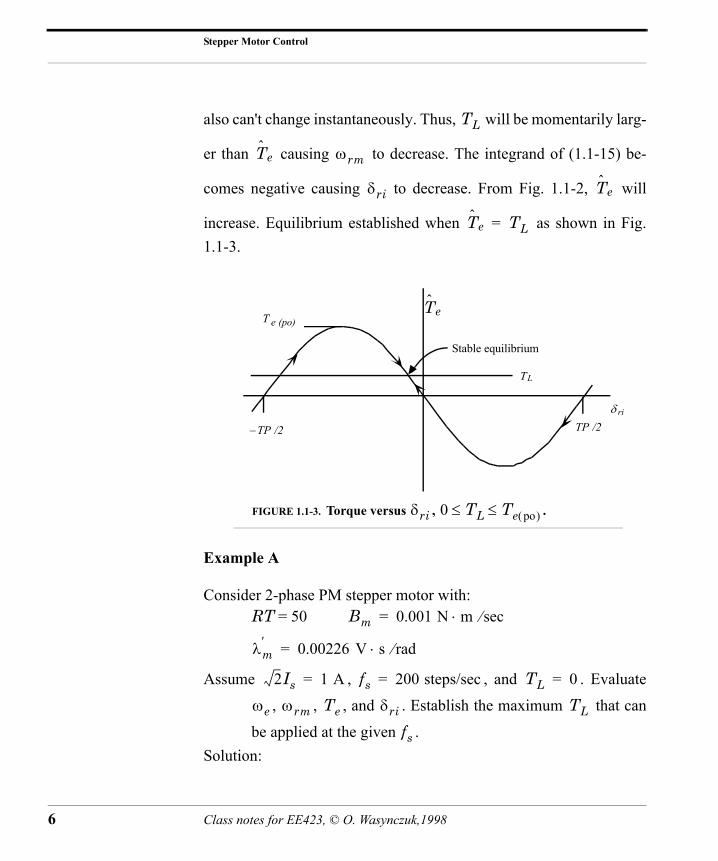
also can't change instantaneously. Thus, will be momentarily larg-

er than causing to decrease. The integrand of (1.1-15) be-

comes negative causing to decrease. From Fig. 1.1-2, will

increase. Equilibrium established when as shown in Fig.1.1-3.

Example A

Consider 2-phase PM stepper motor with:RT = 50

Assume , , and . Evaluate

, , , and . Establish the maximum that can

be applied at the given .Solution:

TL

Te ωrm

δri Te

Te TL=

−TP /2 TP /2δ ri

Stable equilibrium

TL

T e (po)Te

FIGURE 1.1-3. Torque versus , .δri 0 TL Te po( )≤ ≤

Bm 0.001 N m⋅ sec⁄=

λm′ 0.00226 V s⋅ rad⁄=

2Is 1 A= fs 200 steps/sec= TL 0=

ωe ωrm Te δri TL

fs


(A.1)

(A.2)

(A.3)

In the steady state,

= 0 + (0.001)(6.28) = 0.00628 N⋅m (A.4)

(A.5)

⇒

Now and . Thus,

the maximum that can be applied is

for the given .

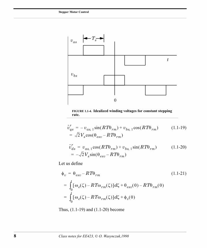
Voltage Controlled DrivesIn an ideal voltage controlled drive, the winding voltages will

be ideal square waves as shown in Fig. 1.1-4. Neglecting harmonics, (1.1-16)

(1.1-17)

where

(1.1-18)

Transforming into the rotor reference frame,

SL 180o

RT( )N------------------- 180o

50( )2-------------- 1.8o= = =

ωeπfs2

------- 3.14( ) 200( )2

----------------------------- 314 rad/sec= = =

ωrmωeRT-------- 314

50--------- 6.28 rad/sec= = =

Te TL Bmωrm+=

Te RTλm′ 2Is RTδri( )sin–

0.113 50δri( )sin– 0.00628 N m⋅

== =

δri 3.2o=

Te po( ) 0.113 N m⋅= Bmωrm 0.00628 N m⋅=

TL 0.113 0.00628– =

0.107 N m⋅ fs

vas 1, 2Vs θesvsin–=

vbs 1, 2Vs θesvcos=

θesv ωe ξ( ) ξd0

t∫ θesv 0( )+=



8

(1.1-19)

(1.1-20)

Let us define

(1.1-21)

Thus, (1.1-19) and (1.1-20) become

vas

vbs

Ts

t

0

FIGURE 1.1-4. Idealized winding voltages for constant stepping rate.

vqsr vas 1, RTθrm( )sin– vbs 1, RTθrm( )cos+

2Vs θesv RTθrm–( )cos=

=

vdsr vas 1, RTθrm( )cos vbs 1, RTθrm( )sin+

2Vs θesv RTθrm–( )sin–=

=

φv θesv RTθrm–

ωe ζ( ) RTωrm ζ( )–[ ] ζd0

t∫ θesv 0( ) RTθrm 0( )–+

ωe ζ( ) RTωrm ζ( )–[ ] ζd0

t∫ φv 0( )+

=

=

=


(1.1-22)

(1.1-23)

These are the same relations as for a brushless dc motor; however, un-like a brushless dc motor, is not under our direct control. What then

determines ? Suppose, for example, that we have a stepper motorwith

RT = 50

Let us determine and the maximum that can be applied.

(1.1-24)

(1.1-25)

With reference to (7.6-9) of EE321 text, (with P/2 replaced by RT and

by

(1.1-26)

vqsr 2Vs φvcos=

vdsr 2Vs φvsin–=

φv

φv

rs 10 Ω=

λm′ 0.00226 V s⋅ rad⁄= Lss 1.1 mH=

fs 300 steps/sec= TL 0=

Vs 10 V(rms)=

φv TL

ωeπfs2

------- 3.14( ) 300( )2

----------------------------- 471 rad/sec= = =

ωrmωeRT-------- 471

50--------- 9.42 rad/sec= = =

ωr RTωrm

Te RTλm

′ rs

rs2 RTωrm( )2Lss

2+------------------------------------------------ Vqs

r RTωrmLssrs

-----------------------------Vdsr– RTωrmλm

′–=



10

(1.1-27)

Equation (1.1-27) is plotted in Fig. 1.1-5. Now, since ,

⇒

(from figure, choose for stable operating point)

Te 50 0.00226( )10

102 50 9.42×( )2 1.1 10 3–×( )2

+----------------------------------------------------------------------------- 14.14 φvcos

50( ) 9.42( ) 1.1 10 3–×( )10

--------------------------------------------------------14.14 φvsin 50 9.42( ) 0.00226( )– –

0.0113 14.14 φvcos 0.773 φvsin– 1.06–[ ]

0.012– 0.16 φv 3°–( )cos+

=

=

=

TL 0=

Te

φv

unstable equilibrium

stable equilibrium

3°

0.148

−0.172

FIGURE 1.1-5. versus at stepping rate of 300 steps/sec.

.

Te φv

T L = 0

φv ωe ζ( ) RTωrm ζ( )–[ ] ζd0

t∫ φv 0( )+=

Te 0 0.012– 0.16 φv 3°–( )cos+= =

φv 85.7° or 88.7°–=

85.7°–


Dynamic response due to change in load torqueSuppose that load torque is stepped to some positive value less

than the maximum shown in Fig. 1.1-5. Since can't change instan-

taneously, will be momentarily greater than . Thus, willdecrease whereby the integrand of (1.1-21) becomes positive. As a re-sult, will increase. The new stable equilibrium point is shown inFig. 1.1-6.

From Fig. 1.1-6, the maximum load torque (including friction)that can be applied at this stepping rate (i.e., the pullout torque) is0.148 N⋅m. The pullout torque may also be established by substituting(1.1-22) and (1.1-23) into (1.1-26), differentiating with respect to ,

setting the result to zero, and solving for . This gives formulas sim-ilar to (7.6-34) and (7.6-35) of the EE321 text, i.e.

(1.1-28)

and

φv

TL Te ωrm

φv

Te

φv

unstable

new equilibrium

3°

0.148

−0.172

TL

FIGURE 1.1-6. versus at stepping rate of 300 steps/sec.

. T e φ v

0 ≤ T L = T e(po )

φv

φv

φv po( ) tan 1– RTωrmτs( )=



12

(1.1-29)

where it is assumed that and are related by

(1.1-30)

Expressing in terms of ,

(1.1-31)

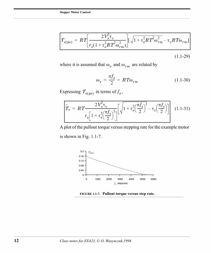
A plot of the pullout torque versus stepping rate for the example motor

is shown in Fig. 1.1-7.

Te po( ) RT2Vs

2τv

rs 1 τs2RT2ωrm

2+( )----------------------------------------------- 1 τs

2RT2ωrm2+ τvRTωrm–[ ]=

ωe ωrm

ωeπfs2

------- RTωrm= =

Te po( ) fs

Te RT2Vs

2τv

rs 1 τs2 πfs

2-------

2

+----------------------------------------- 1 τs

2 πfs2

-------

2+ τv

πfs2

------- –=

Te(po)

fs

FIGURE 1.1-7. Pullout torque versus step rate.


1.2 CONTROL OF PM STEPPER MOTORS

There are two types of stepper motor control systems that we willconsider: fixed and variable rate. The fixed rate control is easier toimplement; however, higher stepping rates can be achived if the step-ping rate is varied.

Fixed stepping rate controlA block diagram of a fixed rate stepper motor control system

is shown in Fig. 1.2-1. Therein, the number of steps to be taken is as-sumed to be known and enterred into an up/down counter that countsthe number of steps to be taken. The excitation sequence generatorsupplies proper excitation to the appropriate stator winding followingeach output clock pulse. In this control, the stepping rate is either zeroor a constant value. The only question we have to answer is: what isthe maximum fixed rate that we can set so that we can be sure thatthere will be no missed steps? This is called the maximum startingrate.

Clock

DownCounter

ExcitationSequenceGenerator

CkStart

-as

+bs

-bs

DriveCircuit

DriveCircuit

start stop

fs

as

vas

ias

ibs

vbs

+

-

+

-

# of steps

# steps

FIGURE 1.2-1. Constant stepping rate open-loop control system.



14

Usually, the starting rate is quite small so that the “back emf”can be neglected whereupon the dynamic equations for phase a maybe expressed

(1.2-1)

The current following a step command resembles that shown in Fig.1.2-2. If, furthermore, , then it is reasonable to neglect .The response then resembles a squre wave as shown in Fig. 1.2-3.

Thus, we can use the static versus characteristics to

vas rs Lssp+( )ias λm′ RTωrm RTθrm( )cos+

rs Lssp+( )ias≈

=

Ts τa» τa

FIGURE 1.2-2. Electrical response for single step,

. λ m' RT ω rm << vas

Vsvas

iasVsrs------

Ts

FIGURE 1.2-3. Electrical response for single step, and .λm

′ RT( )ωrm Vs« Ts τs»

Vsrs------

Vsvas

ias

Ts

Te θrm


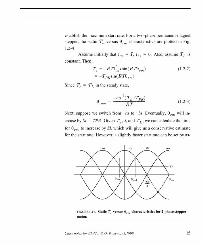
establish the maximum start rate. For a two-phase permanent-magnetstepper, the static versus characteristics are plotted in Fig.1.2-4

Assume initially that , . Also, assume isconstant. Then

(1.2-2)

Since in the steady state,

(1.2-3)

Next, suppose we switch from +as to +bs. Eventually, will in-

crease by SL = TP/4. Given , J, and , we can calculate the time

for to increase by SL which will give us a conservative estimatefor the start rate. However, a slightly faster start rate can be set by as-

Te θrm

+as +bs -bs-as

θrm0 θrm1 θrm

TL

TP4

FIGURE 1.2-4. Static versus characteristics for 2-phase stepper motor.

Te θrm

ias I= ibs 0= TL

Te RTλm′ I RTθrm( )sin–

TPK RTθrm( )sin–=

=

Te TL=

θrmosin 1– TL TPK⁄( )–

RT------------------------------------------=

θrm

Te TL

θrm



16

suming that next step initiated at the crossover angle, . To esti-

mate the time needed to reach , we first calculate the average

torque during the interval from to .

(1.2-4)

Note from Fig. 1.2-4 that . Thus, .

Now, the time needed to reach may be approximated as follows:

(1.2-5)

(1.2-6)

(1.2-7)

(1.2-8)

From which

(1.2-9)

(1.2-10)

where is given by (1.2-4)

θrm1

θrm1

θrm0 θrm1

Te TM1

θrm1 θrm0–------------------------------ TPK RTθrm( )cos θrmd

θrm0

θrm1

∫TPK

RT θrm1 θrm0–( )-------------------------------------------- RTθrm1( )sin RTθrm0( )sin–[ ]

= =

=

θrm1 TP( ) 8⁄= RTθrm1 π 4⁄=

θrm1

d2θrm

dt2---------------- 1

J--- TM TL–( )=

d θ rmdt

=1J

(T M − T L ) t +d θ rm

dt t =0

θ rm =

12 J

(T M − T L ) t2 + θ rm 0

θ rm 1 =

12 J

(T M − T L )T s + θ rm 0

Tsθrm1 θrm0–( )2J

TM TL–------------------------------------------=

fsTM TL–

θrm1 θrm0–( )2J------------------------------------------=

TM


Variable Stepping Rate ControlIn general, a much larger stepping rate can be achieved by

slowly increasing stepping rate to some maximum value and slowlydecreasing it as the target position is approached as shown in Fig. 1.2-5.

In this control strategy, we need to determine:(1) the maximum stepping rate [pullout rate, ](2) the acceleration profile(3) the deceleration profile

In all three cases, we need versus stepping rate characteristic.

If we have a voltage source drive, is given by (1.1-29) or (1.1-31) and plotted in Fig. 1.1-7 for the example machine. If we have acurrent source drive, is given by (1.1-13) and is independent ofstepping rate. In practice, however, constant current cannot be main-tained at large step rates.We typically get something that looks like theplot shown in Fig. 1.2-7. For smaller stepping rates, the pullout torqueis constant. As the stepping rate increases, the back emf increases andthe actual currents may no longer track the desired currents. For veryhigh speeds, the current control degenerates to a voltage control

fs acceleration profile

deceleration profile

constant speed

time

fs (po)

A A = # of steps

FIGURE 1.2-5. Stepping rate versus time.

fs po( )

Te po( )

Te po( )

Te po( )



18

whereupon the pullout torque assymptotically approaches that of avoltage controlled drive. We will find it convenient analytically to ap-proximate the pullout torque versus stepping rate characteristics astwo straigh-line segments, one of which is horizontal.

The maximum stepping rate taht can be achieved is known asthe pullout rate, , which is the intersection of versus

and versus characteristics. To determine acceleration profile,consider mechanical equation

(1.2-11)

For maximum acceleration, assume . Also, assume nomissed steps whereupon

(1.2-12)

Thus

(1.2-13)

0

0.04

0.08

0.12

0.16

0.2

0 1000 2000 3000 4000 5000 6000

TL

Te(po)

f s , steps/sec

fs(po)voltage sou rce

cu rrent sou rce

FIGURE 1.2-6. Extended versus characteristics for current source drive including constraints.

T e(po ) θ rm

fs po( ) Te po( ) fs

TL fs

T e − T L = Jp ω rm

T e = T e(po )

ω rm = SLf s

Te po( ) TL– J SL( )dfsdt--------=


(1.2-14)

Integrating,

(1.2-15)

Dropping subscript 1, the time needed to reach constant stepping rate

of is

(1.2-16)

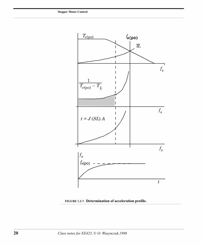
This integral may be integrated graphically or numerically. The se-quence of steps necessary to establish acceleration profile is shown inFig. 1.2-7.

Analytical expressions for the acceleration profile can be de-rived if we can assume is constant and use idealized versus

characteristics shown in Fig. 1.2-8. Let t = time to reach

.

(1.2-17)

(1.2-18)

This implies that we should increase linearly for .

Now let t = time to reach .

dt J SL( ) 1Te po( ) TL–---------------------------- fsd=

t1 td0

t1

∫ J SL( ) 1Te po( ) TL–---------------------------- fsd

0

fs1

∫= =

fs

t J SL( ) 1Te po( ) TL–---------------------------- fsd

0

fs

∫=

TL Te po( )

fs

f s < f s ,bp

t J SL( ) 1Te po( ) TL–---------------------------- fsd

0

fs

∫

SL( )JKfs

=

=

fs1

SL( )JK----------------------t=

fs 0 < f s < f s ,bp

f s ,bp < f s < f s , po



20

TL

Te(po) fs

1Te(po) − TL

A

t = J (SL) A

fs

t

fs

fs

fs

fs

FIGURE 1.2-7. Determination of acceleration profile.


(1.2-19)

TL

fs(po)

fs

1Te(po) - TL

A

fs

fs(bp)

K

Te(po) = C Te(po) = b - a fs

FIGURE 1.2-8. Approximate determination of acceleration profile.

t SL( )J 1Te po( ) TL–---------------------------- fsd

0

fs

∫

SL( )J K fsd0

fs bp,

∫ SL( )J 1b afs– TL–------------------------------ fsd

fs bp,

fs

∫+

tbp SL( )J 1B Afs–------------------- fsd

fs bp,

fs

∫+

tbp SL( )J 1A---- B Afs–( )ln– SL( )J 1

A---- B Afs bp,–( )ln+

=

=

=

=



22

where

(1.2-20)

is the time it takes to increase from 0 to . The approximateoptimum acceleration profile is sketched in Fig. 1.2-9.

tbp SL( )J K fsd0

fs bp,

∫ SL( )JKfs bp,= =

f s f s,bp

linear

exponential

tbp

t

fs,bp

fs,po

fs

FIGURE 1.2-9. Approximate acceleration profile.


chapter 1 stepper motor control - purdue engineeringwasynczu/ee423n/step_motor_control.pdf ·...

Documents