chapter 1 super-resolution: limits and beyond

Chapter 1

SUPER-RESOLUTION: LIMITS AND BEYOND

Simon Bakerand Takeo Kanade

AbstractA variety of super-resolution algorithms have been described in this book.

Most of them are based on the same source of information however; that thesuper-resolution image should generate the lower resolution input images whenappropriately warped and down-sampled to model image formation. (This in-formation is usually incorporated into super-resolution algorithms in the formof reconstruction constraints which are frequently combined with a smoothnessprior to regularize their solution.) In this final chapter, we first investigate howmuch extra information is actually added by having more than one image forsuper-resolution. In particular, we derive a sequence of analytical results whichshow that the reconstruction constraints provide far less useful information as thedecimation ratio increases. We validate these results empirically and show thatfor large enough decimation ratios any smoothness prior leads to overly smoothresults with very little high-frequency content however many (noiseless) low res-olution input images are used. In the second half of this chapter, we propose asuper-resolution algorithm which uses a completely different source of informa-tion, in addition to the reconstruction constraints. The algorithm recognizes local“features” in the low resolution images and then enhances their resolution in anappropriate manner, based on a collection of high and low-resolution trainingsamples. We call such an algorithm ahallucinationalgorithm.

Keywords: Super-resolution, analysis of limits, learning, faces, text, hallucination.

1. INTRODUCTION

A large number of super-resolution algorithms have been described in thisbook. Most of them, however, are based on the same source of information;specifically, that the super-resolution image, when appropriately warped anddown-sampled to model the image formation process, should yield the low res-olution images. This information is typically embedded in a set of reconstruc-tion constraints, first introduced by (Peleg et al., 1987; Irani and Peleg, 1991).

1

2

These reconstruction constraints can be embedded in a Bayesian frameworkincorporating a prior on the super-resolution image (Schultz and Stevenson,1996; Hardie et al., 1997; Elad and Feuer, 1997). Their solution can also beestimated either in batch mode or recursively using a Kalman filter (Elad andFeuer, 1999; Dellaert et al., 1998). Several other refinements have been pro-posed, including simultaneously computing 3D structure (Cheeseman et al.,1994; Shekarforoush et al., 1996; Smelyanskiy et al., 2000) and removing otherdegrading artifacts such as motion blur (Bascle et al., 1996).

In the first part of this chapter, we analyze the super-resolution reconstruc-tion constraints. We derive three analytical results which show that the amountof information provided by having more than one image available for super-resolution becomes very much less as the decimation ratioq increases. Super-resolution therefore becomes inherently much more difficult asq increases.This reduction in the amount of information provided by the reconstructionconstraints is traced to the fact that the pixel intensities in the input imagestake discrete values (typically 8-bit integers in the range 0–255). This causes aloss of information and imposes inherent limits on how well super-resolutioncan be performed from the reconstruction constraints (and other equivalent for-mulations based on the same underlying source of information.)

How, then, can high-decimation ratio super-resolution be performed? Ouranalytical results hold for an arbitrary number of images so using more low res-olution images does not help. Suppose, however, that the input images containprinted text. Moreover, suppose that it is possible to perform optical characterrecognition (OCR) and recognize the text. If the font can also be determined,it would then be easy to perform super-resolution forany decimation ratio.The text could be reproduced at any resolution by simply rendering it fromthe script of the text and the definition of the font. In the second half of thischapter, we describe a super-resolution algorithm based on this idea which wecall hallucination(Baker and Kanade, 1999; Baker and Kanade, 2000a). Oursuper-resolution hallucination algorithm is based, however, on the recognitionof generic local “features” (rather than the characters detected by OCR). It cantherefore be applied to other phenomena such as images of human faces.

2. THE RECONSTRUCTION CONSTRAINTS

Denote the low resolution input images byx(k)L (i; j) wherek = 1; : : : ; K.The starting point in the derivation of the reconstruction constraints is then thecontinuous image formation equation (Horn, 1996):

x(k)L (i; j) =

�I(k)� h

(k)�(i; j) =

Zx(k)L

I(k)(x; y) � h(k)(x� i; y � j) dx dy

(1.1)

Super-resolution: Limits and Beyond 3

S (k)S (k)

* ω (k)I (k)

a (k)

* ω (k)I (k) a (k)* (i,j)I (k)

L(k)x (i,j) = * h (k) (i,j) =

Optical Effects:

I

Spatial Integration:

Lens System

Finite Aperture

CCD Sensor

ω (k)

(k)

Figure 1.1 The low resolution input imagesx(k)L

are formed by the convolution of the irradi-anceI(k) with the camera point spread functionh(k). We model the point spread function itselfas the convolution of two terms: (1)!(k) models the optical effects caused by the lens and thefinite aperture, and (2)a(k) models the spatial integration performed by the CCD sensor.

whereI(k)(x; y) is the continuous irradiance function that would have reachedthe image plane of thekth camera under the pinhole model, andh(k) is pointspread function of thekth camera. The (double) integration is performed overthe image plane ofx(k)L . See Figure 1.1 for an illustration.

2.1 MODELING THE POINT SPREAD FUNCTION

We decompose the point spread function into two parts (see Figure 1.1):

h(k)(x; y) =

�!(k)� a

(k)�(x; y) (1.2)

where!(k)(x; y) models the blurring caused by the optics anda(k)(x; y) mod-

els the spatial integration performed by the CCD sensor (Baker et al., 1998).The optical blurring!(k) is typically further split into a defocus factor that canbe approximated by a pill-box function and a diffraction-limited optical trans-fer function that can be modeled by the square of the first-order Bessel functionof the first kind (Born and Wolf, 1965). We aim to be as general as possible and

4

so avoid making any assumptions about!(k). Instead, (most of) our analysis

is performed for arbitrary optical blurring functions. We do, however, assumea parametric form fora(k). We assume that the the photo-sensitive areas ofthe CCD pixels are square and uniformly sensitive to light, as in (Baker et al.,1998; Barbe, 1980). If the length of the side of the square photosensitive areais S(k), the spatial integration function is then:

a(k)(x; y) =

(1

S(k)�S(k)if jxj � S(k)

2 and jyj � S(k)

2

0 otherwise:(1.3)

In general the photosensitive area is not the entire pixel since space is neededfor the circuitry to read out the charge. Therefore the only assumption we makeaboutS(k) is that it lies in[0; 1]. Our analysis is then in terms ofS(k) (ratherthan the inter-pixel distance which is assumed to define the unit distance.)

2.2 WHAT IS SUPER-RESOLUTION ANYWAY?We wish to estimate a super-resolution imagexH(i

0; j0). Precisely what

does this mean? Let us begin with the coordinate frame ofxH . The coordinateframe of a super-resolution image is typically defined relative to that of thecorresponding low resolution input image. If the decimation ratio isq, thepixels inxH will be q times closer to each other than those in the corresponding

low resolution image,x(k0)

L say. The coordinate frame ofxH can therefore be

defined in terms of that forx(k0)

L via:

(i0; j0) =

�i

q;j

q

�: (1.4)

In this chapter we assume that the input images have already been registeredwith each other and therefore with the coordinate frame ofxH . Then, denotethe point in imagex(k)L (wherek may or may not equalk0) that corresponds to(x; y) in xH by r(k)(x; y). From now on we assume thatr(k) is known.

The integration in Equation (1.1) is performed over the low resolution imageplane. Transforming to the super-resolution image plane ofxH gives:

x(k)L (i; j) =

ZxH

I(k)(r(k)(x; y)) � h(k)(r(k)(x; y)� (i; j)) �

��@r(k)

@x; y

�� dx dy(1.5)

where��@r(k)@x;y

�� is the determinant of the Jacobian of the registrationr(k).

Now, I(k)(r(k)(x; y)) is the irradiance that would have reached the imageplane of thekth camera under the pinhole model, transformed onto the super-resolution image plane. Assuming that the registration is correct, and that theradiance of every point in the scene does change acrossk (a Lambertian-like


assumption),I(k)(r(k)(x; y)) should be the same for allk. Moreover, it equalsthe irradiance that would have reached the super-resolution image plane ofxH

under the pinhole model. Denoting this function byI(x; y), we have:

x(k)L (i; j) =

ZxH

I(x; y) � h(k)(r(k)(x; y)� (i; j)) �

��@r(k)

@x; y

�� dx dy: (1.6)

The goal of super-resolution is then to recover (a representation of)I(x; y).Doing this requires both increasing the resolution and “deblurring” the image;i.e. removing the effects of the convolution with the point spread functionh

(k).In order to proceed we need to specify which continuous functionI(x; y)

is represented by the discrete imagexH(i0; j0). For simplicity, we assume thatxH(i

0; j0) represents the piecewise constant function:

I(x; y) = xH(i0; j0) (1.7)

for all x 2 (i0�0:5; j 0+0:5] andy 2 (j 0�0:5; j0+0:5]. Then, Equation (1.6)can be rearranged to give the super-resolution reconstruction constraints:

x(k)L (i; j) =

Xi0;j0

W(k) �

i; j; i0; j0�� xH(i

0; j0) (1.8)

wherek = 1; : : : ; K and:

W(k) �

i; j; i0; j0� = Z i0+0:5;j0+0:5

i0�0:5;j0�0:5h(k)(r(k)(x; y)� (i; j)) �

��@r(k)

@x; y

�� dx dy:(1.9)

The super-resolution reconstruction constraints are therefore a set of linearconstraints on the unknown super-resolution pixelsxH(i0; j0) in terms of the

known low resolution pixelsx(k)L (i; j) and the coefficientsW (k)(i; j; i0; j0).

3. ANALYSIS OF THE CONSTRAINTS

The constant coefficientsW (k)(i; j; i0; j0) in the reconstruction constraintsdepend on both the point spread functionh

(k) and the registrationr(k). Withoutsome assumptions about these functions any analysis would be meaningless.If the point spread function is arbitrary, it can be chosen to simulate the “smallpixels” of the super-resolution image. Similarly, if the registration is arbitrary,it can be chosen (in effect) to move the camera towards the scene and therebydirectly capture the super-resolution image. We therefore have to make some(reasonable) assumptions about the imaging conditions.

Assumptions Made About the Point Spread FunctionAs mentioned above, we assume that the point spread function takes the

form of Equation (1.3). Moreover, we assume that the width of the photosen-sitive areaS(k) is the same for all of the images (and equalsS.) In the first part

6

of our analysis, we also assume that!(k)(x; y) = �(x) � �(y), where� is the

Dirac delta function. Afterwards, in the second and third parts of our analysis,we allow!(k) to be arbitrary; i.e. our analysis holds foranyoptical blurring.

Assumptions Made About the RegistrationTo outlaw motions which (effectively) allow the camera to be moved to-

wards the scene, we assume that each registration takes the form:

r(k)(x; y) =

1

q(x; y) + (c(k); d(k)) (1.10)

where(c(k); d(k)) is a constant translation (which in general may be differentfor each low resolution imagek) and the1

qaccounts for the change of coordi-

nate frame from high to low resolution images. See also Equation (1.4).Even given these assumptions, the performance of any super-resolution al-

gorithm will depend upon the exact number of input imagesK, the values of(c(k); d(k)), and, moreover, how well the algorithm can register the low res-olution images to estimate the(c(k); d(k)). Our goal is to show that super-resolution becomes fundamentally more difficult as the decimation ratioq in-creases. We therefore assume that the conditions are as favorable as possibleand perform the analysis for an arbitrary number of input imagesK, with arbi-trary translations(c(k); d(k)). We also assume that the algorithm has estimatedthese values perfectly. Any results derived under these conditions will only bestronger in practice, where the registrations may be degenerate or inaccurate.

3.1 INVERTIBILITY ANALYSIS

We first analyze when the reconstruction constraints are invertible, and whatthe rank of the null space is when they are not. In order to get an easily inter-pretable result, the analysis in this section is performed under the scenario thatthe optical blurring can be ignored; i.e.!(k)(x; y) = �(x) � �(y). (This as-sumption will be removed in the following two sections.) The expression forW

(k) (i; j; i0; j 0) in Equation (1.9) then simplifies to:

1

q2

Z i0+0:5

i0�0:5

Z j0+0:5

j0�0:5a(k)

�1

q(x; y) + (c(k); d(k))� (i; j)

�dx dy: (1.11)

Using the definition ofa(k) it can be seen thatW (k) (i; j; i0; j0) is equal to1=(q � S)2 times the area of the intersection of the two squares in Figure 1.2(the high resolution pixel[i0� 0:5; i0+0:5]� [j0� 0:5; j0+0:5] and the regionwherea(k) non-zero and equals1

S2.) We then have:

Theorem 1 If q �S is an integer greater than 1, then for all(c(k); d(k)) the re-construction constraints (Equations (1.8) and (1.11)) are not invertible. More-over, the dimension of the null space is at least(q � S � 1)2. If q � S is not aninteger,c(k) andd(k) always exist such that the constraints are invertible.


1D Proof

Area A

(i’-0.5,j’-0.5)

(i’+0.5,j’+0.5)

(c , d )(k)(k)q((i,j) - + S (0.5,0.5))

(c , d )(k)(k) - S (0.5,0.5))q((i,j) -

Figure 1.2 The high-resolution pixel(i0; j0) over which the integration is performed in Equa-tion (1.11) is indicated by the small square at the upper middle left of the figure. The largersquare towards the bottom right is the region in whicha(k) is non-zero. Sincea(k) takes thevalue1=S2 in this region, the integral in Equation (1.11) equalsA=S2, whereA is the area ofthe intersection of the two squares. This figure is used to illustrate the 1D proof of Theorem 1.

Proof: We provide a proof for 1D images. (See Figure 1.2.) The extension to2D is conceptually no more difficult and so is omitted for reasons of brevity.

The null space is defined byP

i0;j0 W(k)

(i; j; i0; j0) � x(k)H (i0; j0) = 0 where

W(k)

(i; j; i0; j 0) = (q �S)2 �W (k)(i; j; i0; j0) is the area of intersection of the 2squares in Figure 1.2. Any element of the null space therefore corresponds toan assignment of values to the small squares such that their weighted sum (overthe large square) equals zero, where the weights are the areas of intersection.

In 1D we just consider one row of the figure. Changingc(k) (andd(k))

to slide the large square along the row by a small amount, we get a similarconstraint on the elements in the null space. The only difference is in the left-most and right-most small squares. Subtracting these two constraints showsthat the left-most square and the right-most square must have the same value.

If q � S is not an integer (or is 1), this proves that neighboring values ofx(k)H

must be equal and hence0. (Sinceq � S is not an integer, the big square slidesout of one small square before the other and the result then follows by transitiv-ity of equality.) Therefore, there exist values for the translationsc

(k) (andd(k))such that the null space only contains the zero vector; i.e. the reconstructionconstraints are invertible in general ifq � S is not an integer (or is 1).

If q � S is an integer greater than1, this same constraint places an upperbound ofq �S�1 on the maximum dimension of the null space computed overall possible translationsc(k) (andd(k)). The space of all assignments tox(k)H

8

(a) q = 2:0 (b) q = 1:5 (c) q = 2:0, with Prior

Figure 1.3 Validation of Theorem 1: The results of solving the reconstruction constraints usinggradient descent for a square point spread function withS = 1:0. (a) Whenq � S is an integer,the equations are not invertible and so a random periodic image in the null space is added tothe original image. (b) Whenq � S is not an integer, the reconstruction constraints are invertible(in general) and so a smooth solution is found, even without a prior. (The result forq = 1:5was interpolated to make it the same size as that forq = 2:0.) (c) When a smoothness prior isadded to the reconstruction constraints the difficulties seen in (a) disappear. (For larger valuesof q simply adding a smoothness prior does not solve this problem, as will be seen.)

that are periodic with periodq � S and which have a zero mean can also easilybe seen to always lie in the null space and so this value is also a lower boundon the dimension of the null space for any translationsc

(k) (andd(k)). 2

To validate this theorem, we solved the reconstruction constraints using gra-dient descent for the two casesq = 2:0 andq = 1:5, (whereS = 1:0.) Theresults are presented in Figure 1.3. In this experiment, no smoothness prior isused and gradient descent is run for a sufficiently long time that the (smooth)initial image does not bias the results. The input in both cases consisted of mul-tiple down-sampled images of the face. Specifically,1024 randomly translatedimages were used as input. Exactly the same inputs are used for the two exper-iments. The only difference is the decimation ratio. (The output forq = 1:5 isactually smaller than that forq = 2:0 and was interpolated to be the same sizefor display purposes. This is the reason it appears slightly smoother than (c).)

As can be seen in Figure 1.3, forq = 2:0 the (additive) error is approxi-mately a periodic image with period2 pixels. Forq = 1:5 the equations areinvertible and so a smooth solution is found, even though no smoothness priorwas used. Forq = 2:0, the fact that the problem is not invertible does nothave any practical significance. Adequate solutions can be obtained by simplyadding a smoothness prior to the reconstruction constraints, as shown in Fig-ure 1.3(c). Forq � 2 the situation is different, however. The rapid rate ofincrease of the dimension of null space (quadratic inq � S) is the root cause ofthe problems, as will be seen in the next two sections.


3.2 CONDITIONING ANALYSIS

Most linear systems that are close to being not invertible are usually ill-conditioned. It is no surprise then that changing from a square point spreadfunction to an arbitrary blurring functionh(k) = !

(k) � a(k) results in an ill-conditioned system, as we now show in the second part of our analysis:

Theorem 2 If !(k)(x; y) is a function for which!(k)(x; y) � 0 for all (x; y)and

R R!(k)(x; y) dx dy = 1, then the condition number of the reconstruction

constraints (Equations (1.8) and (1.9)) grows at least as fast as(q � S)2.

Proof: We first prove the theorem for the square point spread functionh(k) =

a(k) (i.e. for Equations (1.8) and (1.11)) and then generalize. The condition

number of a linear operatorA can be written as:

Cond(A) =supkxk1=1 kAxk1

infkxk1=1 kAxk1: (1.12)

It follows from Equations (1.8) and (1.11) that ifxH(i0; j0) = 1 for all (i0; j0),

thenx(k)L (i; j) = 1 for all (i; j). Hence the numerator in Equation (1.12) is atleast1. SettingxH(i0; j0) to be the checkerboard pattern (1 ifi0 + j

0 is even,

-1 if odd) we find thatjx(k)L (i; j)j � 1=(q � S)2 since the integration of thecheckerboard over any square in the real plane lies in the range[�1; 1]. (Proofomitted.) Hence the denominator is at most1=(q � S)2. The desired result forh(k) = a

(k) follows immediately.For arbitrary point spread functions, note that Equations (1.8) and (1.9) can

be combined and then rewritten as:

x(k)L (i; j) =

ZxH

xH(x; y)

q2� h

(k)�1

q(x; y) + (c(k); d(k))� (i; j)

�dx dy

=�h(k)� xH

�((c(k); d(k))� (i; j))

=h!(k)�

�a(k)� xH

�i((c(k); d(k))� (i; j)) (1.13)

where we have setxH(x; y) = xH(�qx;�qy) and changed variables(x; y))

�1q(x; y). Both of the properties ofx(k)L that we used to prove the result for

square point spread functions therefore also hold witha(k) replaced byh(k) =

!(k) � a(k) using standard properties of the convolution operator. Hence, the

desired, more general, result follows immediately from Equation (1.13).2This theorem is more general than the previous one because it applies to

arbitrary optical blurring functions. On the other hand, it is a weaker result (insome situations)because it only predicts that super-resolution isill-conditioned(rather than not invertible.) This theorem on its own, therefore, does not en-tirely explain the poor performance of super-resolution. As we showed in Fig-ure 1.3, problems that are ill-conditioned (or even not invertible, where the

10

condition number is infinite) can often be solved by simply adding a smooth-ness prior. (The not invertible super-resolution problem in Figure 1.3(a) issolved in Figure 1.3(c) in this way.) Several researchers have performed con-ditioning analysis of various forms of super-resolution, including (Elad andFeuer, 1997; Shekarforoush, 1999; Qi and Snyder, 2000). Although useful,none of these results fully explain the drop-off in performance with the deci-mation ratioq. The weakness of conditioninganalysis is that an ill-conditionedsystem may be ill-conditioned because of a single “almost singular value.” Asindicated by the rapid growth in the dimension of the null space in Theorem 1,super-resolution has a large number of “almost singular values” for largeq.This is the real cause of the difficulties seen in Figure 1.4, as we now show.

3.3 ANALYSIS OF THE VOLUME OF SOLUTIONS

If we could work with noiseless, real-valued quantities and perform arbitraryprecision arithmetic then the fact that the reconstruction constraints are ill-conditioned might not be a problem. In reality, however, images are alwaysintensity discretized (typically to 8-bit values in the range 0–255 grey levels.)There will therefore always be noise in the measurements, even if it is onlyplus-or-minus half a grey-level. Suppose thatint[�] denotes the operator whichtakes a real-valued irradiance measurement and turns it into an integer-valuedintensity. If we incorporate this quantization into our image formation model,the reconstruction constraints in Equation (1.13) become:

x(k)L (i; j) = int

�ZxH

xH(x; y)

q2h(k)

�1

q(x; y) + (c(k); d(k))� (i; j)

�dx dy

�:

(1.14)Suppose also thatxH is a finite size image withn pixels. We then have:

Theorem 3 The volume of solutions of the intensity discretized reconstructionconstraints in Equation (1.14) grows asymptoticallyat least as fast as(q�S)2�n.

Proof: First note that the space of solutions is convex since integration is linear.Next note that one solution of Equation (1.14) is the solution of:

x(k)L (i; j)� 0:5 =

ZxH

xH(x; y)

q2h(k)

�1

q(x; y) + (c(k); d(k))� (i; j)

�dx dy:

(1.15)The definition of the point spread function ash(k) = !

(k) � a(k) and the prop-erties of the convolution give0 � h

(k) � 1=S2. Therefore, adding(q � S)2 toany pixel inxH is still a solution since the right hand side of Equation (1.15)increases by at most 1. (The integrand is increased by less than1 grey-level inthe pixel, which only has an area of1 unit.) The volume of solutions of Equa-tion (1.14) therefore contains ann-dimensional simplex, where the angles at


No. Inputs 4 16 64 256

Decimationq 2 4 8 16

Figure 1.4 Results of the reconstruction-based super-resolution algorithm (Hardie et al., 1997)for various decimation ratios. A high high-resolution image of a face is translated multiple timesby random sub-pixel amounts, blurred with a Gaussian, and then down-sampled. (The algorithmis provided with exact knowledge of the point spread function and the sub-pixel translations.)Comparing the images in the right-most column, we see that the algorithm does quite well giventhe very low resolution of the input. The degradation in performance as the decimation ratioincreases from left to right is very dramatic, however.

one vertex are all right-angles, and the sides are all(q � S)2 units long. Thevolume of such a simplex grows asymptotically like(q � S)2n (treatingn as aconstant andM andS as variables). The desired result follows. 2

In Figures 1.4 and 1.5 we present results to illustrate Theorems 2 and 3. Wetook a high resolution image of a face and translated it by random sub-pixelamounts, blurred it with a Gaussian, and then down-sampled it. We repeatedthis procedure for several decimation ratios;q = 2, 4, 8, and 16. In each case,we generated multiple down-sampled images,each with a different translation.We generated enough images so that there were as many low resolution pixelsin total as pixels in the original high resolution image. For example, we gener-ated 4 half size images, 16 quarter size images, and so on. We then applied thealgorithms of (Hardie et al., 1997) and (Schultz and Stevenson, 1996).

The results for (Hardie et al., 1997) are shown in the figure. The resultsfor (Schultz and Stevenson, 1996) were very similar and are omitted. We pro-vided the algorithms with exact knowledge of both the point spread functionused in the down-sampling and the random sub-pixel translations. Restrictingattention to the right-most column of Figure 1.4, the results look very good.

12

0

20

40

60

80

100

2 4 6 8 10 12 14 16

RM

S In

tens

ity D

iffer

ence

in G

rey-

Leve

ls

Decimation Ratio

Reconstruction ErrorResidual Error

Single Image Interpolation ErrorPredicted Error

Sup

er-R

es.

Sm

ooth

ness

Prio

r

Figure 1.5 An illustration of Theorems 2 and 3 using the same inputs as in Figure 1.4. Thereconstruction error is much higher than the residual, as would be expected for an ill-conditionedsystem. For low decimation ratios, the prior is unnecessary and so the results are worse thanpredicted. For high decimation ratios, the prior does help, but at the price of smooth results.(See Figure 1.4.) An estimate of the amount of information provided by the reconstructionconstraints is given by the improvement of the reconstruction error over the interpolation error.Similarly, the improvement from the predicted error to the reconstruction error is an estimate ofthe amount of information provided by the smoothness prior. By this measure, the smoothnessprior provides more information than the reconstruction constraints forq = 16.

The algorithm is able to do a decent job of reconstructing the face from inputimages which barely resemble faces. On the other hand, the performance getsmuch worse as the decimation ratio increases (from left to right.)

Our third and final theorem provides the best explanation of these results.For large decimation ratiosq = 8 and16, there is a huge volume of solutions tothe discretized reconstruction constraints in Equation (1.14). The smoothnessprior which is added to resolve this ambiguity simply ensures that it is one ofthe overly smooth solutions that is chosen. (Of course, without the prior anysolution might be chosen which would generally be even worse.)

Using the same inputs as Figure 1.4, we plot the reconstruction error againstthe decimation ratio in Figure 1.5; i.e. the difference between the reconstructedhigh resolution image and the original. We compare this error with the resid-ual error; i.e. the difference between the low resolution inputs and their pre-dictions from the reconstructed high resolution image. As expected for an ill-conditioned system, the reconstruction error is much higher than the residual.We also compare with a rough prediction of the reconstruction error obtained


by multiplying the lower bound on the condition number(q � S)2 by an es-timate of the expected residual assuming that the grey-levels are discretizedfrom a uniform distribution. For low decimation ratios, this estimate is anunder-estimate because the prior is unnecessary for noise free data; i.e. betterresults would be obtained without the prior. For high decimation ratios theprediction is an over-estimate because the local smoothness assumption doeshelp the reconstruction (albeit at the expense of overly smooth results.)

We also plot interpolation results in Figure 1.5; i.e. just using the recon-struction constraints for one image (as was proposed, for example, in (Schultzand Stevenson, 1994).) The difference between this curve and the reconstruc-tion error curve is a measure of how much information the reconstruction con-straints provide. Similarly, the difference between the predicted error and thereconstruction error is a measure of how much information the smoothnessprior provides. For a decimation ratio of16, we see that the prior providesmore information than the super-resolution reconstruction constraints.

4. SUPER-RESOLUTION BY HALLUCINATIONHow then is it possible to perform super-resolution with a high decimation

ratio without the results looking overly smooth? As we have just shown, the re-quired high-frequency information was lost from the reconstruction constraintswhen the input images were discretized to 8-bit values. Smoothness priors mayhelp regularize the problem, but cannot replace the missing information.

Our goal in this section is to develop a super-resolution algorithm whichuses the information contained in a collection of recognition decisions (in ad-dition to the reconstruction constraints.) Our approach (which we callhallu-cination) is to embed the results of the recognition decisions in arecognition-based prioron the solution of the reconstruction constraints, thereby hopefullyresolving the inherent ambiguity in their solution.

Our approach is somewhat related to that of (Freeman and Pasztor, 1999)who recently, and independently, proposed a learning framework for low-levelvision, one application of which is image interpolation. Besides being ap-plicable to an arbitrary number of images, the other major advantage of ourapproach is that it uses a prior which is specific to the class of object (in the“class-based” sense of (Riklin-Raviv and Shashua, 1999)) and a set of localrecognition decisions. Our algorithm is also related to (Edwards et al., 1998),in which active-appearance model are used for model-based super-resolution.

4.1 BAYESIAN MAP FORMULATION

We use a Bayesian formulation of super-resolution (Cheeseman et al., 1994;Schultz and Stevenson, 1996; Hardie et al., 1997; Elad and Feuer, 1997). Inthis approach, super-resolution is posed as finding the maximuma posteriori

14

(or MAP) super-resolution imagexH : i.e. estimatingargmaxxH P [xH j x(k)L ].

Bayes law for this estimation problem is:

P [xH j x(k)L ] =

P [x(k)L j xH] � P [xH ]

P [x(k)L ]

: (1.16)

SinceP [x(k)L ] is a constant because the imagesx(k)L are (known) inputs, and

since the logarithm function is a monotonically increasing function, we have:

argmaxxH

P [xH j x(k)L ] = argmin

xH

�� lnP [x

(k)L j xH]� lnP [xH ]

�: (1.17)

The first term in this expression� ln P [x(k)L j xH ] is the (negative log) prob-

ability of reconstructing the low resolution imagesx(k)L given that the super-resolution image isxH . It is therefore normally set to be a quadratic (i.e. en-ergy) function of the error in the reconstruction constraints:

� ln P [x(k)L j xH ] =

1

2�2�

Xi;j;k

24x(k)L (i; j)�

Xi0;j0

W(k) �

i; j; i0; j0�� xH(i

0; j0)

352

(1.18)whereW (k)(i; j; i0; j 0) is defined in Equation (1.9). In this expression, we areimplicitly assuming that the noise is independently and identically distributed(across both the images and the pixels) and is Gaussian with covariance�

2�.

4.2 RECOGNITION-BASED PRIORSThe second term on the right-hand side of Equation (1.17) is (the nega-

tive logarithm of) the prior� lnP [xH ]. Usually the prior is chosen to bea simple smoothness prior (Cheeseman et al., 1994; Schultz and Stevenson,1996; Hardie et al., 1997; Elad and Feuer, 1997). Instead, we would like it todepend upon the results of a set of recognition decisions. Suppose the outputsof the recognition decisions partition the inputs (i.e. the low resolution inputimagesx(k)L ) into a set of subclassesfCk;l j l = 1; 2; : : :g: We then define arecognition-based prioras one that can be written in the following form:

P [xH ] =Xl

P [xH j x(k)L 2 Ck;l] � P [x

(k)L 2 Ck;l]: (1.19)

Essentially there is a separate priorP [xH j x(k)L 2 Ck;l] for each possible par-

tition Ck;l of the input space. Once the low resolution input imagesx(k)L are

available, the various recognition algorithms can be applied, and it can be de-termined which partition the inputs lie in. The recognition-based priorP [xH ]

then reduces to the more specific priorP [xH j x(k)L 2 Ck;l]. This prior can be

made more powerful than the overall prior because it can be tailored toCk;l.


G 0

G 1

G 3

G 2

G 4

Parent Structure vector PS 2

L 0

L 1

L 3

L 2

L 4

V0

V1

V3

V2

V4

H 0

H 1

H 3

H 2

H 4

(a) Gaussian Pyramid (b) Laplacian Pyramid (c) First Derivative Pyramids

Figure 1.6 The Gaussian, Laplacian, and first derivative pyramids of an image of a face. (Wealso use two second derivatives but omit them from the figure.) We combine these pyramidsinto a single multi-valued pyramid, where we store a vector of the Laplacian and the derivativesat each pixel. The Parent Structure vectorPSl(i; j) of a pixel (i; j) in the lth level of thepyramid consists of the vector of values for that pixel, the vector for its parent in thel + 1th

level, the vector for its parent’s parent, etc (De Bonet, 1997). The Parent Structure vector istherefore a high-dimensionalvector of derivatives computed at various scales. In our algorithms,recognition means finding the training sample with the most similar Parent Structure vector.

4.3 MULTI-SCALE DERIVATIVE FEATURES

We decided to try to recognize generic local image features (rather thanhigher level concepts such as ASCII characters) because we want to apply ouralgorithm to a variety of phenomena. Motivated by (De Bonet, 1997), we alsodecided to use multi-scale features. In particular, given an imagex, we firstform its Gaussian pyramidG0(x); : : : ; GN(x) (Burt, 1980). Afterwards, wealso form its Laplacian pyramidL0(x); : : : ; LN(x) (Burt and Adelson, 1983),the horizontalH0(x); : : : ; HN(x) and verticalV0(x); : : : ; VN(x) first deriva-tives of the Gaussian pyramid, and the horizontalH

20(x); : : : ; H

2N(x) and ver-

ticalV 20 (x); : : : ; V

2N(x) second derivatives of the Gaussian pyramid. (See Fig-

ure 1.6 for examples of these pyramids.) Finally, we form a feature pyramid:

Fj(x) =�Ll(x); Hl(x); Vl(x); H

2l (x); V

2l (x)

�for l = 0; : : : ; N: (1.20)

The pyramidF0(x); : : : ;FN(x) is a pyramid where there are 5 values storedat each pixel, the Laplacian and the 4 derivatives.

Then, given a pixel in the low resolution image that we are performingsuper-resolution on, we want to find (i.e. recognize) a pixel in a collectionof training data that is locally “similar.” By similar, we mean that both theLaplacian and the image derivatives are approximately the same, at all scales.To capture this notion, we define the Parent Structure vector (De Bonet, 1997)of a pixel(i; j) in thelth level of the feature pyramidF0(x); : : : ;FN(x) to be:

16

PS 2

x(k)Lx(k)

L( )

x(k)L( )

x(k)L( )

x(k)L( )PS 2

x(k)Lx(m)

T

x(m)T( )

x(m)T( )

x(m)T( )

x(m)T( )

x(m)T( )

x(m)T( )

F

F

F

F

F

F

F

F

0

1

2

3

4

Low-Resolution Input Image

2

3

4

Recognition Output

Best Image Best Pixel

BI BP

Match

=

(k)(k)

High-Resolution Training Images

Figure 1.7 We compute the feature pyramidsF0(x(m)T

); : : : ;FN (x(m)T

) for the training im-

agesx(m)T

and the feature pyramidsFl(x(k)L

); : : : ;FN(x(k)L

) for the low resolution input images

x(k)L

. For each pixel in the low resolution images, we find (i.e. recognize) the closest matchingParent Structure in the high resolution data. We record and output the best matching imageBI(k) and the pixel location of the best matching Parent StructureBP

(k). Note that these datastructures are both defined independently for each pixel(i; j) in each imagex(k)

L.

PSl(x)(i; j) =�Fl(x)(i; j);Fl+1(x)(

�i

2

�;

�j

2

�); : : : ;FN(x)(

�i

2N�l

�;

�j

2N�l

�):

�(1.21)

As illustrated in Figure 1.6, the Parent Structure vector at a pixel in the pyramidconsists of the feature vector at that pixel, the feature vector of the parent ofthat pixel, the feature vector of its parent, and so on. Exactly as in (De Bonet,1997), our notion of two pixels being similar is then that their Parent Structurevectors are approximately the same (measured by some norm.)

4.4 FINDING THE CLOSEST PARENT STRUCTURE

Suppose we have a set of high resolution training imagesx(m)T wherem =

1; 2; : : : ;M . We first form the feature pyramidsF0(x(m)T ); : : : ;FN(x

(m)T ).

Also suppose that the input imagex(k)L is at a resolution that isq = 2l timessmaller than the training samples. (The image may have to be interpolated tomake this ratio exactly a power of 2.) We can then compute the feature pyra-mid for the input image from levell and upwardsFk(x

(k)L ); : : : ;FN(x

(k)L ).

Figure 1.7 shows an illustration of this scenario forl = 2.Independently for each pixel(i; j) in the inputx(k)L , we compare its Parent

Structure vectorPSl(x(k)L )(i; j)against all of the training Parent Structure vec-

tors at the same levell; i.e. we compare againstPSl(x(m)T )(i0; j0) for all m and

for all (i0; j 0). The best matching imageBI(k)(i; j) = m and the best matchingpixel BP(k)(i; j) = (i0; j0) are stored as the output of the recognition deci-


sion, independently for each pixel(i; j) in x(k)L . (We found the performance

to be largely independent of the distance function used to determine the bestmatching Parent Structure vector. We actually used a weightedL2-norm, giv-ing the derivative components half as much weight as the Laplacian values andreducing the weight by a factor of2 for each increase in the pyramid level.)

Recognition in our hallucination algorithm therefore means finding the clos-est matching pixel in the training data in the sense that the Parent Structurevectors of the the two pixels are the most similar. This search is, in general,performed over all pixels in all of the images in the training data. If we havefrontal images of faces, however, we restrict this search to consider only thecorresponding pixels in the training data. In this way, we treat each pixel inthe input image differently, depending on its spatial location, similarly to the“class-based” approach of (Riklin-Raviv and Shashua, 1999).

4.5 THE RECOGNITION-BASED GRADIENT PRIORFor each pixel(i; j) in the input imagex(k)L , we have recognized the pixel

that is the most similar in the training data, specifically, the pixelBP(k)(i; j)

in the lth level of the pyramid for training imagex(BI(k)(i;j))

T . These recogni-tion decisions partition the inputs into a collection of subclasses, as requiredby the recognition-based prior described in Section 4.2. If we denote the sub-classes byC

k;BP(k);BI(k) (i.e. using a multi-dimensional index rather thanl)Equation (1.19) can be rewritten as:

P [xH ] =X

BP(k);BI(k)

P [xH j x(k)L 2 C

k;BP(k);BI(k) ] � P [x(k)L 2 C

k;BP(k);BI(k) ]

(1.22)whereP [xH j x

(k)L 2 C

k;BP(k);BI(k) ] is the probability that the super-resolution

image isxH , given that the inputsx(k)L lie in the subclass that will be recog-

nized to haveBP(k) as the best matching pixel in training imagex(BI(k)(i;j))

T .

We now need to defineP [xH j x(k)L 2 C

k;BP(k);BI(k) ]. We decided to makethis recognition-based prior a function of the gradient because the base, or aver-age, intensities in the super-resolution image are defined by the reconstructionconstraints. It is the high-frequency gradient information that is missing. So,we want to define the prior to encourage the gradient of the super-resolutionimage to be close to the gradient of the closest matching training samples.

Each low resolution input imagex(k)L has a (different) closest matching (Par-ent Structure) training sample for each pixel. Moreover, each such ParentStructure corresponds to a number of different pixels in the0th level of thepyramid, (2l of them to be precise. See also Figure 1.7.) We therefore imposea separate gradient constraint for each pixel(i; j) in the0th level of the pyra-

18

mid (and for each input imagex(k)L .) The best matching pixelBP(k) is onlydefined on thelth level of the pyramid. For notational convenience, therefore,given a pixel(i; j) on the0th level of the pyramid, define the best matchingpixel on the0th level of the pyramid to be:

BP(k)

(i; j) � 2l �BP(k)(

�i

2l

�;

�j

2l

�) + (i; j)� 2l � (

�i

2l

�;

�j

2l

�): (1.23)

Also define the best matching image asBI(k)

(i; j)� BI(k)(ji2l

k;

jj

2l

k).

If (i; j) is a pixel in the0th level of the pyramid for imagex(k)L , the cor-

responding pixel in the super-resolution imagexH is�r(k)��1

( i2l;j

2l). We

therefore want to impose the constraint that the first derivatives ofxH at thispoint should equal the derivatives of the closest matching pixel (Parent Struc-ture) in the training data. Parametric expressions forH0(xH) andV0(xH) at�r(k)��1

( i2l;j

2l) can easily be derived as linear functions of the unknown pix-

els in the high resolution imagexH . We assume that the errors in the gradientvalues between the recognized training samples and the super-resolution im-age are independently and identically distributed and moreover that they areGaussian with covariance�2r. Therefore:P [xH j x

(k)L 2 C

k;BP(k);BI(k) ] =

1

2�2r

0@Xi;j;k

�H0(xH)(

�r(k)��1

(i

2l;j

2l))�H0(x

BI(k)

(i;j)T )(BP

(k)(i; j))

�2

Xi;j;k

�V0(xH)(

�r(k)��1

(i

2l;j

2l))� V0(x

BI(k)

(i;j)T )(BP

(k)(i; j))

�21A :

(1.24)

This prior enforces the constraints that the gradient of the super-resolution im-agexH should equal to the gradient of the best matching training image.

4.6 ALGORITHM PRACTICALITIES

Equations (1.17), (1.18), (1.22), and (1.24) form a high-dimensional lin-ear least squares problem. The constraints in Equation (1.18) are the standardsuper-resolution reconstruction constraints. Those in Equation (1.24) are therecognition-based prior. The relative weights of these constraints are definedby the noise covariances�2� and�2r. We assume that the reconstruction con-straints are the more reliable ones and so set�

2� � �

2r.

The number of unknowns is equal to the number of pixels inxH . Inverting alinear system of such a size can prove problematic. We therefore implemented


a gradient descent algorithm using the standard diagonal approximation to theHessian (Press et al., 1992) to set the step size in a similar way to (Szeliski andGolland, 1998). Since the error function is quadratic, the algorithm convergesto the (single) global minimum without any problem.

4.7 EXPERIMENTAL RESULTS ON HUMAN FACES

Our experiments for human face images were conducted with a subset ofthe FERET dataset (Philips et al., 1997) consisting of 596 images of 278 indi-viduals (92 women and 186 men). Most people appear twice, with the imagestaken on the same day under similar illumination conditions, but with differ-ent expressions (one expression is neutral, the other typically a smile.) A smallnumber of people appear 4 times, with the images separated by several months.

The images in the FERET dataset are256 � 384 pixels, however the areaoccupied by the face varies considerably, but most of the faces are around96�

128 pixels or larger. In the class-based approach (Riklin-Raviv and Shashua,1999), the input images (which are all frontal) need to be aligned so that wecan assume that the same part of the face appears in roughly the same partof the image every time. This alignment was performed by hand marking thelocation of 3 points, the centers of the two eyes and the lower tip of the nose.These 3 points define an affine warp (Bergen et al., 1992), which was used towarp the images into a canonical form. These canonical96�128 pixel imageswere then used as the training samplesx

(m)T wherem = 1; : : :596.

We used a “leave-one-out” methodology to test our algorithm. To test onany particular person, we removed all occurrences of that individual from thetraining set. We then trained the algorithm on the reduced training set, andtested on the images of the individual that had been removed. Because thisprocess is quite time consuming, we used a test set of 100 randomly selectedimages of 100 different individuals rather than the entire training set.

Comparison with Existing Super-Resolution AlgorithmsWe initially restrict attention to the case of enhancing24� 32 pixel images

four times to give96� 128 pixel images. Later we will consider the variationin performance with the decimation ratio. We simulate the multiple slightlytranslated images required for super-resolution using the FERET database byrandomly translating the original FERET images multiple times by sub-pixelamounts before down-sampling them to form the low resolution input images.

In our first set of experiments we compare our algorithm with those of(Hardie et al., 1997) and (Schultz and Stevenson, 1996). In Figure 1.8(a) weplot the RMS pixel error against the number of low resolution inputs, computedover the 100 image test set. (We compute the RMS error using the original highresolution image used to synthesize the inputs from.) We also plot results forcubic B-spline interpolation (which only uses one image) for comparison.

20

10

15

20

25

30

1 10

RM

S E

rror

Per

Pix

el in

Gre

y-Le

vels

Number of Input Images

Cubic B-splineHallucinationHardie et al.

Schultz and Stevenson

10

15

20

25

30

35

40

0 2 4 6 8 10 12 14 16

RM

S E

rror

Per

Pix

el in

Gre

y-Le

vels

Standard Deviation of Additive Noise

Cubic B-splineHallucinationHardie et al.

Schultz and Stevenson

(a) Variation with the Number of Images (b) Variation with Additive Noise

Figure 1.8 A comparison of our hallucination algorithm with the reconstruction-based super-resolution algorithms of (Schultz and Stevenson, 1996) and (Hardie et al., 1997). In (a) weplot the RMS pixel intensity error computed across the 100 image test set against the numberof low resolution input images. Our algorithm outperforms the the traditional super-resolutionalgorithms across the entire range. In (b) we vary the amount of additive noise. Again we findthat our algorithm does better than the traditional super-resolution algorithms.

(a) Input24� 32 (b) Hallucinated (c) Hardieet al. (d) Original

(d) Input24� 32 (e) Hallucinated (f) Hardieet al. (g) Original

Figure 1.9 The best and worst results in Figure 1.8(a) in terms of the RMS error of the hallu-cination algorithm for 9 input images. In (a)–(d) we display the results for the best performingimage in the 100 image test set. The results for the worst image are presented in (e)–(g). (Theresults for Schultz and Stevenson are similar to those for Hardieet al. and are omitted.) Thereis little difference in image quality between the best and worst hallucinated results.


(a) Std. Dev. 2.0 (b) Std. Dev. 4.0 (c) Std. Dev. 8.0 (d) Std. Dev. 16.0

Figure 1.10 An example from Figure 1.8(b) of the variation in the performance of the halluci-nation algorithm with additive zero-mean, white Gaussian noise. As can be seen, the output ishardly affected until around 4-bits of intensity noise have been added to the inputs. The reasonthe hallucination algorithm is so robust to noise it that it uses the strong recognition-based faceprior to generate smooth, face-like images however noisy the inputs are.

In Figure 1.8(a) we see that our hallucination algorithm does outperformthe reconstruction-based super-resolution algorithms, from one input image to25. The improvement is consistent across the number of input images and isaround 20%. The improvement is also largely independent of the actual input.In particular, Figure 1.9 contains the best and worst results obtained across theentire test set in terms of the RMS error of the hallucination algorithm for 9low resolution inputs. As can be seen, there is little difference between the bestresults in Figure 1.9(a)–(d) and the worst ones in (e)–(g). Notice, also, how thehallucinated results are a dramatic improvement over the low resolution input,and moreover are visibly sharper than the results for Hardieet al..

Robustness to Additive Intensity NoiseFigure 1.8(b) contains the results of an experiment investigating the robust-

ness of the 3 super-resolution algorithms to additive noise. In this experiment,we added zero-mean, white Gaussian noise to the low resolution images be-fore passing them as inputs to the algorithms. In the figure, the RMS pixelintensity error is plotted against the standard deviation of the additive noise.The results shown are for 4 low resolution input images, and again, the re-sults are an average over the 100 image test set. As might be expected, theperformance of all 4 algorithms gets much worse as the standard deviationof the noise increases. The hallucination algorithm and cubic B-spline inter-polation, however, seem somewhat more robust than the reconstruction-basedsuper-resolution algorithms. The reason for this increased robustness is proba-bly that the hallucination algorithm always tends to generate smooth, face-likeimages (because of the strong recognition-based prior) however noisy the in-puts are. One example of how the hallucination algorithm degrades with theamount of additive noise is presented in Figure 1.10.

22

Input 48� 64 24� 32 12� 16

Output �2 �4 �8

Reduction in 77% 56% 57%

RMS error vs.

cubic B-spline (9.2 vs. 11.9) (12.4 vs. 22.2) (19.5 vs. 33.9)

Figure 1.11 The variation in the performance of our hallucination algorithm with the inputimage size. We see that the algorithm works well down to12 � 16 pixel images. It begins tobreak down for6� 8 pixel images. See (Baker and Kanade, 1999) for examples.

Variation in Performance with the Input Image SizeWe do not expect our hallucination algorithm to work for all sizes of input.

Once the input gets too small, the recognition decisions will be based on es-sentially no information. In the limit that the input image is just a single pixel,the algorithm will always generate the same face (for a single input image),but with different average grey levels. We therefore investigated the lowestresolution at which our hallucination algorithm works reasonable well.

In Figure 1.11 we show example results for one face in the test set for 3different input sizes. (All of the results use just 4 input images.) We see thatthe algorithm works reasonably well down to12� 16 pixels. (For6� 8 pixelimages it produces a face that appears to be a pieced-together combination ofa variety of faces. See (Baker and Kanade, 1999) for examples.)

In the last row of Figure 1.11, we give numerical results of the averageimprovement in the RMS error over cubic B-spline interpolation (computed


(a) Input12� 16 (b) Hallucinated (d) Original (e) Cubic B-spline

Figure 1.12 Selected results for12 � 16 pixel images, the smallest input size for which ourhallucination algorithm works reliably. (The input consists of only 4 low resolution input im-ages.) Notice how sharp the hallucinated results are. See (Baker and Kanade, 1999) for theresults of (Hardie et al., 1997) which are omitted due to lack of space.

24

Cropped Cubic B-spline Hallucinated

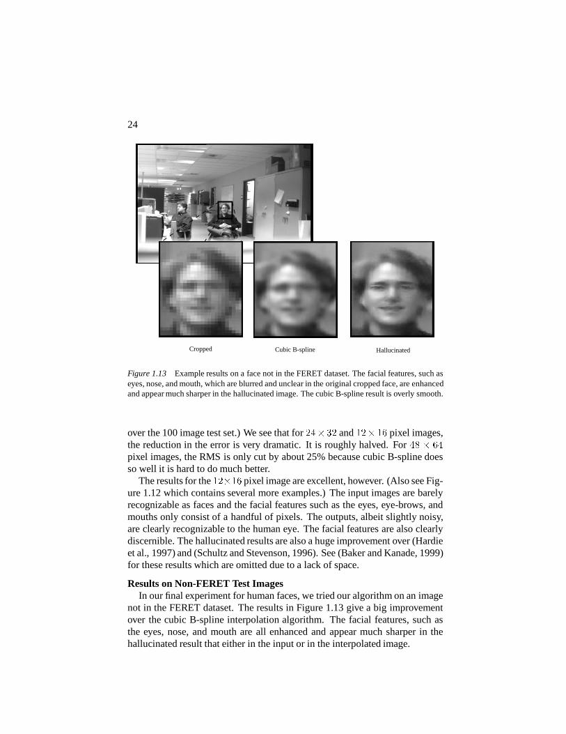
Figure 1.13 Example results on a face not in the FERET dataset. The facial features, such aseyes, nose, and mouth, which are blurred and unclear in the original cropped face, are enhancedand appear much sharper in the hallucinated image. The cubic B-spline result is overly smooth.

over the 100 image test set.) We see that for24� 32 and12� 16 pixel images,the reduction in the error is very dramatic. It is roughly halved. For48 � 64

pixel images, the RMS is only cut by about 25% because cubic B-spline doesso well it is hard to do much better.

The results for the12�16 pixel image are excellent, however. (Also see Fig-ure 1.12 which contains several more examples.) The input images are barelyrecognizable as faces and the facial features such as the eyes, eye-brows, andmouths only consist of a handful of pixels. The outputs, albeit slightly noisy,are clearly recognizable to the human eye. The facial features are also clearlydiscernible. The hallucinated results are also a huge improvement over (Hardieet al., 1997) and (Schultz and Stevenson, 1996). See (Baker and Kanade, 1999)for these results which are omitted due to a lack of space.

Results on Non-FERET Test ImagesIn our final experiment for human faces, we tried our algorithm on an image

not in the FERET dataset. The results in Figure 1.13 give a big improvementover the cubic B-spline interpolation algorithm. The facial features, such asthe eyes, nose, and mouth are all enhanced and appear much sharper in thehallucinated result that either in the input or in the interpolated image.


(a) Miscellaneous (b) Hallucinated (c) Constant (d) Hallucinated

Figure 1.14 The results of applying our algorithm to images not containing faces. (We haveomitted the low resolution input and just display the high resolution one.) A face is hallucinatedby our algorithm even when none is present, hence the term “hallucination.”

Results on Images Not Containing FacesIn Figure 1.14 we briefly present a few results on images that do not contain

faces, even though the algorithm has been trained on the FERET dataset. (Fig-ure 1.14(a) is a miscellaneous image and Figure 1.14(c) is a constant image.)As might be expected, our algorithm hallucinates an outline of a face in bothcases, even though there is no face in the input. This is the reason we calledour algorithm a “hallucination algorithm.”

4.8 EXPERIMENTAL RESULTS ON TEXT DATAWe also applied our algorithm to text data. In particular, we grabbed an

image of an window displaying one page of a letter and used the bit-map as theinput. The image was split into disjoint training and test samples. The resultsare presented in Figures 1.15. The input in Figure 1.15(a) is half the resolutionof the original in Figure 1.15(f). The hallucinated result in Figure 1.15(c) is thebest reconstruction of the text, both visually and in terms of the RMS intensityerror. For example, compare the appearance of the word “was” in the secondsentence in Figures 1.15(b)–(f). The hallucination algorithm also has an RMSerror of only 24.5 grey levels, compared to over 48.0 for the other algorithms.

5. SUMMARY

In the first half of this chapter we showed that the super-resolution recon-struction constraints provide less and less useful information as the decimationratio increases. The major cause of this phenomenon is the spatial averagingover the photosensitive area; i.e. the fact thatS is non-zero. The underlyingreason that there are limits on reconstruction-based super-resolution is there-fore the simple fact that CCD sensors must have a non-zero photosensitive areain order to be able to capture a non-zero number of light photons.

26

(a) Input Image. (Just one image is used.)

(b) Cubic B-spline, RMS Error 51.3

(c) Hallucinated, RMS Error 24.5x

(d) Schultz and Stevenson, RMS Error 48.4

(e) Hardieet al., RMS Error 48.5

(f) Original High Resolution Image

Figure 1.15 The results of enhancing the resolution of a piece of text by a factor of 2. Ourhallucination algorithm produces a clear, crisp image using no explicit knowledge that the inputcontains text. In particular, look at the word “was” in the second sentence. The RMS pixelintensity error is also almost a factor of 2 improvement over the other algorithms.


Our analysis assumes quantized noiseless images; i.e. the intensities are8-bit values, created by rounding noiseless real-valued numbers. (It is thisquantization that causes the loss of information, which when combined withspatial averaging, means that high decimation ratio super-resolution is not pos-sible from the reconstruction constraints.) Without this assumption, however,it might be possible to increase the number of bits per pixel by averaging a col-lection of quantized noisy images (in an intelligent way). In practice, takingadvantage of such information is very difficult. This point also does not affectanother outcome of our analysis which was to show that reconstruction-basedsuper-resolution inherently trades-off intensity resolution for spatial resolution.

In the second half of this chapter we showed that recognition processes mayprovide an additional source of information for super-resolution algorithms.In particular, we developed a “hallucination” algorithm and demonstrated thatthis algorithm can obtain far better results than existing reconstruction-basedsuper-resolution algorithms, both visually and quantitatively.

6. DISCUSSION

In the past 10-15 years or so much of the research on super-resolution hasfocused on the reconstruction constraints, and various way of incorporatingsimple smoothness priors to allow the constraints to be solved. It is a majoraccomplishment that most of this area is now fairly well understood. This doesnot mean that super-resolution is now a “solved” problem. As we have shownin this chapter, simply writing down the reconstruction constraints, adding asmoothness prior, and solving the resulting linear system does not necessarilymean that a good solution will be found. There are therefore a number of wideopen areas for future super-resolution research:

One such area involves conducting detailed analysis of the reconstruc-tion constraints, when they provide additional information, how muchadditional information they provide, and how sensitive the informationis to the signal to noise ratio of the input images. Some preliminary workhas been done in this area, including (Elad and Feuer, 1997; Shekar-foroush, 1999; Qi and Snyder, 2000; Baker and Kanade, 2000b). How-ever, many issues are still a long way from being fully understood.

Much of the work on super-resolution assumes a fairly simple imageformation model. For example, there is almost no modeling of the effectof non-Lambertian surfaces and varyingillumination. As a result, manyalgorithms (including the one described in this chapter) are very sensitiveto illumination effects such as shadowing. Although some illuminationinvariant super-resolution algorithms have been proposed (Chiang andBoult, 1997), much more work remains to be done.

28

In the second half of this chapter we proposed a hallucination algorithm.This algorithm is an instance of a model-based algorithm. Other exam-ples include (Edwards et al., 1998; Freeman and Pasztor, 1999; Bakerand Kanade, 2000a). These approaches appear very promising, howeverthe area of model-based super-resolution is in its infancy and a great dealof work remains to be done for completely exploit the idea.

Other areas which have been largely overlooked include the investiga-tion of applications of super-resolution and the evaluation of the util-ity of super-resolution algorithms for those applications. There are twotypes of applications: (1) those where the enhanced image will be shownto a human, and (2) those where the enhanced image will be further pro-cessed by a machine. The evaluation of these two types of applicationswill be very different. The first will need to be done using rigoroussubjective studies of how humans can make use of the super-resolutionimages. The second use of super-resolution is best evaluated in termsof the performance of the algorithms that will actually use the enhancedimages. Both of these areas have barely been touched, even though theyare vital for proving the utility of super-resolution as a whole.

Acknowledgements

We wish to thank Harry Shum for pointing out the reference (Freeman andPasztor, 1999), Iain Matthews for pointing out (Edwards et al., 1998), andHenry Schneiderman for suggesting the conditioning analysis in Section 3.2.We would also like to thank a number of people for comments and sugges-tions, including Terry Boult, Peter Cheeseman, Michal Irani, Shree Nayar,Steve Seitz, Sundar Vedula, and everyone in the Face Group at CMU. Theresearch described in this chapter was supported by US DOD Grant MDA-904-98-C-A915. A preliminary version of this chapter appeared in the IEEEConference on Computer Vision and Pattern Recognition (Baker and Kanade,2000b). More experimental results can be found in (Baker and Kanade, 1999).

References

Baker, S. and Kanade, T. (1999). Hallucinating faces. Technical Report CMU-RI-TR-99-32, The Robotics Institute, Carnegie Mellon University.

Baker, S. and Kanade, T. (2000.a). Hallucinating faces. InProceedings of theFourth International Conference on Automatic Face and Gesture Recogni-tion, Grenoble, France.

Baker, S. and Kanade, T. (2000b). Limits on super-resolution and how to breakthem. InProceedings of the 2000 IEEE Conference on Computer Vision andPattern Recognition, Hilton Head, South Carolina.


Baker, S., Nayar, S., and Murase, H. (1998). Parametric feature detection.In-ternational Journal of Computer Vision, 27(1):27–50.

Barbe, D. (1980).Charge-Coupled Devices. Springer-Verlag.Bascle, B., Blake, A., and Zisserman, A. (1996). Motion deblurring and super-

resolution from an image sequence. InProceedings of the Fourth EuropeanConference on Computer Vision, pages 573–581, Cambridge, England.

Bergen, J. R., Anandan, P., Hanna, K. J., and Hingorani, R. (1992). Hierarchi-cal model-based motion estimation. InProceedings of the Second EuropeanConference on Computer Vision, pages 237–252, Santa Margherita Liguere,Italy.

Born, M. and Wolf, E. (1965).Principles of Optics. Permagon Press.Burt, P. (1980). Fast filter transforms for image processing.Computer Graphics

and Image Processing, 16:20–51.Burt, P. and Adelson, E. (1983). The Laplacian pyramid as a compact image

code.IEEE Transactions on Communiations, 31(4):532–540.Cheeseman, P., Kanefsky, B., Kraft, R., Stutz, J., and Hanson, R. (1994). Super-

resolved surface reconstruction from multiple images. Technical Report FIA-94-12, NASA Ames Research Center, Moffet Field, CA.

Chiang, M.-C. and Boult, T. (1997). Local blur estimation and super-resolution.In Proceedings of the 1997 Conference on Computer Vision and PatternRecognition, pages 821–826, San Juan, Puerto Rico.

De Bonet, J. (1997). Multiresolution sampling procedure for analysis and syn-thesis of texture images. InComputer Graphics Proceedings, Annual Con-ference Series, (SIGGRAPH ’97), pages 361–368.

Dellaert, F., Thrun, S., and Thorpe, C. (1998). Jacobian images of super-resolvedtexture maps for model-based motion estimation and tracking. InProceed-ings of the Fourth Workshop on Applicationsof Computer Vision, pages 2–7,Princeton, NJ.

Edwards, G., Taylor, C., and Cootes, T. (1998). Learning to identify and trackfaces in image sequences. InProceedings of the Third International Con-ference on Automatic Face and Gesture Recognition, pages 260–265, Nara,Japan.

Elad, M. and Feuer, A. (1997). Restoration of single super-resolution imagefrom several blurred, noisy and down-sampled measured images.IEEE Trans-actions on Image Processing, 6(12):1646–58.

Elad, M. and Feuer, A. (1999). Super-resolution reconstruction of image se-quences.IEEE Transactions on Pattern Analysis and Machine Intelligence,21(9):817–834.

Freeman, W. and Pasztor, E. (1999). Learning low-level vision. InProceedingsof the Seventh InternationalConference on Computer Vision, Corfu, Greece.

30

Hardie, R., Barnard, K., and Armstrong, E. (1997). Joint MAP registration andhigh-resolution image estimation using a sequence of undersampled images.IEEE Transactions on Image Processing, 6(12):1621–1633.

Horn, B. (1996).Robot Vision. McGraw Hill.Irani, M. and Peleg, S. (1991). Improving resolution by image restoration.

Computer Vision, Graphics, and Image Processing, 53:231–239.Peleg, S., Keren, D., and Schweitzer, L. (1987). Improving image resolution

using subpixel motion.Pattern Recognition Letters, pages 223–226.Philips, P., Moon, H., Rauss, P., and Rizvi, S. (1997). The FERET evaluation

methodology for face-recognition algorithms. InCVPR ’97.Press, W., Teukolsky, S., Vetterling, W., and Flannery, B. (1992).Numerical

Recipes in C. Cambridge University Press, second edition.Qi, H. and Snyder, Q. (2000). Conditioning analysis of missing data estimation

for large sensor arrays. InProceedings of the 2000 IEEE Conference onComputer Vision and Pattern Recognition, Hilton Head, South Carolina.

Riklin-Raviv, T. and Shashua, A. (1999). The Quotient image: Class basedrecognition and synthesis under varying illumination. InProceedings of the1999 Conference on Computer Vision and Pattern Recognition, pages 566–571, Fort Collins, CO.

Schultz, R. and Stevenson, R. (1994). A Bayseian approach to image expansionfor improved definition.IEEE Transactions on Image Processing, 3(3):233–242.

Schultz, R. and Stevenson, R. (1996). Extraction of high-resolution framesfrom video sequences.IEEE Transactions on Image Processing, 5(6):996–1011.

Shekarforoush, H. (1999). Conditioningbounds for multi-frame super-resolutionalgorithms. Technical Report CAR-TR-912, Computer Vision Laboratory,Center for Automation Research, University of Maryland.

Shekarforoush, H., Berthod, M., Zerubia, J., and Werman, M. (1996). Sub-pixel bayesian estimation of albedo and height.International Journal ofComputer Vision, 19(3):289–300.

Smelyanskiy, V., Cheeseman, P., Maluf, D., and Morris, R. (2000). Bayesiansuper-resolved surface reconstruction from images. InProceedings of the2000 IEEE Conference on Computer Vision and Pattern Recognition, HiltonHead, South Carolina.

Szeliski, R. and Golland, P. (1998). Stereo matching with transparency andmatting. InSixth International Conference on Computer Vision (ICCV’98),pages 517–524, Bombay.

chapter 1 super-resolution: limits and beyond

Documents