chapter 10: detection and attribution of climate … · 2 chapter 10: detection and attribution of...
TRANSCRIPT

First Order Draft Chapter 10 IPCC WGI Fifth Assessment Report
Do Not Cite, Quote or Distribute 10-1 Total pages: 138
1
Chapter 10: Detection and Attribution of Climate Change: from Global to Regional 2 3 Coordinating Lead Authors: Nathaniel Bindoff (Australia), Peter Stott (UK) 4 5 Lead Authors: Krishna Mirle AchutaRao (India), Myles Allen (UK), Nathan Gillett (Canada), David 6 Gutzler (USA), Kabumbwe Hansingo (Zambia), Gabriele Hegerl (UK), Yongyun Hu (China), Suman Jain 7 (Zambia), Igor Mokhov (Russia), James Overland (USA), Judith Perlwitz (USA), Rachid Sebbari (Morocco), 8 Xuebin Zhang (Canada) 9 10 Contributing Authors: Ping Chang, Tim DelSole, Catia M. Domingues, Paul J. Durack, Alexey Eliseev, 11 Chris Forest, Hugues Goosse, Jara Imbers Quintana, Gareth S. Jones, Georg Kaser, Reto Knutti, James 12 Kossin, Mike Lockwood, Fraser Lott, Jian Lu, Irina Mahlstein, Damon Matthews, Seung-Ki Min, Thomas 13 Moelg, Simone Morak, Friederike Otto, Debbie Polson, Andrew Schurer, Tim Osborn , Joeri Rogelj, 14 Vladimir Semenov, Dmitry Smirnov, Peter Thorne, Rong Zhang 15 16 Review Editors: Judit Bartholy (Hungary), Robert Vautard (France), Tetsuzo Yasunari (Japan) 17 18 Date of Draft: 16 December 2011 19 20 Notes: TSU Compiled Version 21 22
23 Table of Contents 24 25 Executive Summary..........................................................................................................................................326 10.1Introduction ..............................................................................................................................................627 10.2Evaluation of Detection and Attribution Methodologies ......................................................................728
10.2.1The Context of Detection and Attribution .......................................................................................829 Box 10.1: How Attribution Studies Work ......................................................................................................930
10.2.2Time-Series Methods, Granger Causality and Methods Separating Signal and Noise by 31 Timescale or Spatial Scale .......................................................................................................................1132 10.2.3Methods Based on General Circulation Models and Optimal Fingerprinting .............................1133 10.2.4Single-Step and Multi-Step Attribution .........................................................................................1334 10.2.5Linking Detection and Attribution to Model Evaluation and Prediction: Bayesian and 35 Frequentist Approaches and the Role of the Null-Hypothesis .................................................................1336
10.3Atmosphere and Surface........................................................................................................................1437 10.3.1Temperature ..................................................................................................................................1438 10.3.2Water Cycle...................................................................................................................................2639 10.3.3Climate Phenomena ......................................................................................................................3140
10.4Changes in Ocean Properties ................................................................................................................3441 10.4.1Ocean Temperature and Heat Content .........................................................................................3542 10.4.2Ocean Salinity and Freshwater Fluxes .........................................................................................3643 10.4.3Sea Level .......................................................................................................................................3844 10.4.4Oxygen ..........................................................................................................................................3945
10.5Cryosphere ..............................................................................................................................................3946 10.5.1Sea Ice ...........................................................................................................................................3947 10.5.2 Ice Sheets, Ice Shelves, and Glaciers ............................................................................................4248 10.5.3Snow Cover and Permafrost .........................................................................................................4449
10.6Extremes ..................................................................................................................................................4450 10.6.1Attribution of Changes in Frequency/Occurrence and Intensity of Extremes ..............................4551 10.6.2Attribution of Observed Weather and Climate Events..................................................................5052
10.7Multi Century to Millennia Perspective ...............................................................................................5353 10.7.1Relevance of and Challenges in Detection and Attribution Studies Prior to the 20th Century....5354 10.7.2Causes of Change in Large-Scale Temperature Over the Past Millennium.................................5455 10.7.3Changes of Past Regional Temperature .......................................................................................5656 10.7.4Causes or Contributors to Change in Specific Periods ................................................................5657

First Order Draft Chapter 10 IPCC WGI Fifth Assessment Report
Do Not Cite, Quote or Distribute 10-2 Total pages: 138
10.7.5Changes in Regional Precipitation, Drought and Circulation .....................................................581 10.7.6Estimates of Unforced Internal Climate Variability .....................................................................582 10.7.7Summary: Lessons from the Past ..................................................................................................583
10.8Whole System Attribution .....................................................................................................................594 10.8.1Multivariable Studies ....................................................................................................................595 10.8.2Earth System Analysis ...................................................................................................................606
10.9Implications for Climate System Properties and Projections ............................................................617 10.9.1Transient Climate Response..........................................................................................................618 10.9.2Magnitude of Precipitation Response ...........................................................................................639 10.9.3Constraints on Long Term Climate Change and the Equilibrium Climate Sensitivity .................6410 10.9.4Consequences for Aerosol Forcing and Ocean Heat Uptake .......................................................6811 10.9.5Earth System Properties................................................................................................................6912
FAQ 10.1: Climate is Always Changing. How do We Determine the Most Likely Causes of the 13 Observed Changes? ................................................................................................................................6914
FAQ 10.2: When will Human Influences on Climate be Obvious on Local Scales? ................................7115 References........................................................................................................................................................7516 Tables .............................................................................................................................................................10017 Figures ...........................................................................................................................................................113 18
19

First Order Draft Chapter 10 IPCC WGI Fifth Assessment Report
Do Not Cite, Quote or Distribute 10-3 Total pages: 138
Executive Summary 1 2 Evidence of the effects of human influence on the climate system has continued to accumulate and 3 strengthen since the AR4. The consistency of observed and modeled changes across the climate system, 4 including regional temperatures, the water cycle, global energy budget, cryosphere and oceans, points to a 5 large-scale warming resulting primarily from anthropogenic increases in greenhouse gas concentrations. 6 7 Evidence for Warming 8 The anthropogenic fingerprints in the surface temperature (including over land and water), in the free 9 atmosphere (cooling in the stratosphere and warming in the troposphere) and in the ocean (warming 10 spreading from the surface to depth) are expected to be distinctive in their patterns in space and time from 11 the dominant modes of decadal variability and the expected response to changes in solar output and 12 explosive volcanic eruptions. Quantification of the contributions of anthropogenic and natural forcing using 13 multi-signal detection and attribution analyses show with (very high confidence) that it is very likely that 14 most of the observed increase in global average temperatures since the mid-20th century is due to the 15 observed anthropogenic increase in greenhouse gas concentrations. Other forcings, including variability in 16 tropospheric and stratospheric aerosols, stratospheric water vapour, and solar output, as well as internal 17 modes of variability, have contributed to the year to year and decade to decade variability of the climate 18 system. It is very likely that early 20th century warming is due in part to external forcing. It is extremely 19 likely that warming since 1950 cannot be explained without external forcing. It is very likely that global 20 temperature changes since 1998 are consistent with an on-going anthropogenic greenhouse gas induced 21 warming trend, and the response to other known forcings. 22 23 More than 90% of the earth’s radiative imbalance is taken up by the oceans through increased subsurface 24 temperatures. It is virtually certain that the most of the rise in ocean temperatures observed since the 1970s is 25 caused by external forcing. This ocean warming is also causing thermal expansion and it is virtually certain 26 that there is an anthropogenic influence on the global steric sea level rise for this period. 27 28 The fingerprint of human activity has emerged in observed temperature changes of the free atmosphere. It is 29 likely that the warming of the troposphere is attributable to anthropogenic forcings dominated by greenhouse 30 gases. It is very likely that the cooling of the lower stratosphere is attributable to anthropogenic forcing 31 dominated by ozone depleting substances. The pattern of tropospheric warming and stratospheric cooling 32 observed since 1960 is very likely to be due to the influence of anthropogenic forcings. 33 34 The Water Cycle 35 New evidence has emerged for the detection of anthropogenic influence on aspects of the water cycle. While 36 observational and modelling uncertainties remain, the consistency of the evidence from both atmosphere and 37 ocean points to anthropogenic influence on the water cycle. This is seen in the detection of human influence 38 on zonal patterns of global precipitation changes, on high northern latitude precipitation changes, and on 39 atmospheric humidity in multiple datasets, together with expectations from theoretical considerations and 40 systematic changes observed in oceanic surface and sub-surface salinity. These patterns are consistent with 41 an amplified global water cycle. There is medium confidence that there is a significant human influence on 42 global scale changes in precipitation patterns, including reductions in low latitudes and increases in northern 43 hemisphere mid to high latitudes. Remaining observational uncertainties and the large effect of natural 44 variability on observed precipitation preclude a more confident assessment at this stage. An anthropogenic 45 contribution to increases in tropospheric specific humidity is found with medium confidence. It is likely (high 46 confidence) that observed changes in ocean surface and sub-surface salinity are due in part to anthropogenic 47 increases in greenhouse gases. 48 49 The Cryosphere 50 Reductions in Arctic sea ice and northern hemisphere snow cover extent, permafrost degradation and glacier 51 retreat and increased surface melt of Greenland are evidence of systematic changes in the cryosphere linked 52 to anthropogenic climate change. It is likely that anthropogenic forcings have contributed to Arctic sea ice 53 retreat (high confidence) and the increased surface melt of Greenland. The small net change in Antarctic sea 54 ice extent appears consistent with the combined effects of anthropogenic and natural forcings and variability 55 (medium confidence). It is likely that there has been an anthropogenic component to observed reductions in 56 snow cover and permafrost. It is likely that glaciers have diminished significantly due to human influence 57

First Order Draft Chapter 10 IPCC WGI Fifth Assessment Report
Do Not Cite, Quote or Distribute 10-4 Total pages: 138
since the 1960s. Due to a low level of scientific understanding there is very low confidence that observed loss 1 of Antarctic ice sheet mass balance is caused by anthropogenic forcing. 2 3 Climate Extremes 4 There has been a strengthening of the evidence for human influence on temperature extremes since the AR4. 5 It is very likely that anthropogenic forcing has affected the frequency of extreme temperatures over land 6 around the globe. It is likely that human influence has significantly increased the probability of some 7 observed heatwaves. There is medium confidence that anthropogenic forcing has contributed to a trend 8 towards increases in the frequency of heavy precipitation events over the second half of the 20th century 9 over land regions with sufficient observational coverage to make the assessment. There is low confidence in 10 attribution of changes in tropical cyclone activity to human influence due to insufficient observational 11 evidence and a low level of scientific understanding. 12 13 From Global to Regional 14 Further evidence has accumulated on the detection and attribution of anthropogenic influence on climate 15 change in different parts of the world. Over every continent except Antarctica, anthropogenic influence has 16 likely made a substantial contribution to surface temperature increases, and – with medium confidence - has 17 made a significant contribution to warming in Antarctica. It is likely that there has been significant 18 anthropogenic warming in Arctic land surface temperatures over the past 50 years. Detection and attribution 19 at regional scales due to greenhouse gases is complicated by the greater role played by dynamical factors 20 (circulation changes) and a greater range of forcings that may be regionally important. Nevertheless, human 21 influence on temperature in some subcontinental regions is likely detectable. 22 23 Changes in atmospheric circulation are important for local climate change since they could act to reinforce or 24 counteract the effects of external forcings on climate in a particular region. There is medium confidence for 25 an anthropogenic influence on the observed widening of the tropical belt which has resulted in a poleward 26 expansion of the Hadley circulation. It is likely that there has been an anthropogenic contribution to the 27 trends in the Southern Annular Mode which correspond to sea level pressure reductions over the high 28 latitudes, an increase in the subtropics, and a southward shift of the storm tracks. There is medium confidence 29 that changes in the Northern Atlantic Oscillation, are consistent with natural internal variability. Differences 30 between the hemispheres are consistent with the greater role of ozone depletion in the Southern Hemisphere. 31 32 A Millennia to Multi-Century Perspective 33 Taking a longer term perspective shows the substantial role played by external forcings in driving climate 34 variability on hemispheric scales, even in pre-industrial times. While internal variability of the climate 35 system, with its ability to move heat around the climate system is important at hemispheric scales, it is very 36 unlikely that reconstructed temperatures since 1400 can be explained by natural internal variability alone. 37 Climate model simulations that include only natural forcings can explain a substantial part of the pre-38 industrial inter-decadal temperature variability on hemispheric scales. However such simulations fail to 39 explain more recent warming without the inclusion of anthropogenic increases in greenhouse gas 40 concentrations. 41 42 Implications for Climate System Properties and Projections 43 More observational data have allowed a better characterisation of basic properties of the climate system 44 which have implications for the rate of future warming. New evidence from 21st century observations that 45 were not yet available to AR4 indicates that the transient climate response (TCR) is estimated to be very 46 likely greater than 1°C, and very unlikely greater than 3ºC. This observation-based range for TCR is smaller 47 than estimated at the time of AR4, due to the stronger observational constraints and the wider range of 48 studies now available. The global warming response to carbon dioxide emissions has been found to be 49 determined primarily by total cumulative emissions of carbon dioxide, irrespective of the timing of those 50 emissions over a broad range of scenarios. The ratio of warming to cumulative emissions, the Transient 51 Climate Response to Cumulative Carbon Emissions is estimated to be very likely between 1°C/TtC and 52 3°C/TtC based on observational constraints. Estimates based on observational constraints continue to 53 indicate that it is very likely that the equilibrium climate sensitivity is larger than 1.5°C. Evidence from 54 observations also supports the overall assessment that climate sensitivity is likely in the range from 2–4.5°C. 55 56 Remaining Uncertainties 57

First Order Draft Chapter 10 IPCC WGI Fifth Assessment Report
Do Not Cite, Quote or Distribute 10-5 Total pages: 138
At regional scales considerable challenges remain in attributing observed change to external forcing. 1 Modelling uncertainties related to model resolution and incorporation of relevant processes become more 2 important at regional scales, and the effects of internal variability become more significant in masking or 3 enhancing externally forced changes. Observational uncertainties for climate variables and forcings such as 4 aerosols, and limits in process understanding continue to hamper attribution of changes in many aspects of 5 the climate system, making it more difficult to discriminate between natural internal variability and 6 externally forced changes. Increased understanding of uncertainties in radiosonde and satellite records makes 7 assessment of causes of observed trends in the upper troposphere less confident than an assessment of overall 8 atmospheric temperature changes. Changes in the water cycle remain less reliably modelled in both their 9 changes and their internal variability, limiting confidence in attribution assessments. The ability to simulate 10 changes in frequency and intensity of extreme events is limited by the ability of models to reliably simulate 11 mean changes in key features of circulation such as blocking and to simulate soil moisture feedbacks. 12
13

First Order Draft Chapter 10 IPCC WGI Fifth Assessment Report
Do Not Cite, Quote or Distribute 10-6 Total pages: 138
10.1 Introduction 1 2 This chapter seeks to understand the causes of the observed changes that were assessed in Chapters 2 to 5. 3 The chapter uses physical understanding, climate models and statistical approaches to assess the causes of 4 observed climate changes. It assesses whether changes in climate can be detected as being significantly 5 outside the range expected from natural internal variability and assesses to what extent observed changes can 6 be attributed to external drivers of climate change, both human induced and naturally occurring. It looks 7 across the climate system as a whole, assessing whether there are coherent changes being observed that are 8 consistent with current understanding of how the global climate is expected to behave, and assesses the 9 implication for climate projections. The chapter also takes a regional perspective in assessing why changes 10 differ from place to place across the planet. 11 12 To achieve its objectives, this chapter looks right across the climate system, from the upper atmosphere to 13 beneath the surface of the ocean. Its remit goes beyond temperature to assess also changes in the water cycle, 14 circulation and climate phenomena (Section 10.3), ocean properties, including ocean temperature and salinity 15 and sea level (Section 10.4), and the cryosphere, including sea ice, ice sheets, ice shelves and glaciers, and 16 snow cover and permafrost (Section 10.5). The chapter considers not just how mean climate has changed but 17 also how extremes are changing (Section 10.6) and, while it has a particular focus on the period for which 18 instrumental data are available it also takes a multi-century perspective, including using non-instrumental 19 data from paleoclimate archives (Section 10.7). It also considers the implications of new understanding of 20 observed changes for climate projections both on the near-term and the long-term (Section 10.9). 21 22 There is increased focus on the extent to which the climate system as a whole is responding in a coherent 23 way across a suite of climate indices such as surface mean temperature, temperature extremes, ocean heat 24 content, river run off and precipitation change. A whole system perspective is taken in section 10.8 which 25 makes a synthesis of the evidence presented throughout the chapter for human influence on climate. 26 27 Research on the impacts of observed changes is assessed by Working Group II, which includes a chapter on 28 detection and attribution of impacts. We adopt the terminology proposed by the IPCC good practice 29 guidance paper on attribution (Hegerl et al., 2010) in describing the different approaches to attribution 30 practised in the literature. Methodological approaches to detection and attribution are evaluated in Section 31 10.2. 32 33 There are additional challenges for detection and attribution in proceeding from global to regional scales. 34 Distinguishing signals of externally forced climate changes from the noise of natural internal variability 35 generally becomes more difficult as spatial scale reduces. There is incomplete observational coverage of 36 climate going back in time and observational uncertainties can be a greater problem for some regions than 37 others. Models need to be assessed for their reliability at representing climate variability and change in the 38 particular region in question, and local forcings such as changes in land use, that have little effect on large 39 scales, may be important on regional scales. Extremes may be infrequently observed and dynamical or 40 statistical models may be required to characterise the underlying variability of such rare events. 41 42 Evidence of a human influence on climate has progressively accumulated during the period of the four 43 previous assessment reports of the IPCC. There was little observational evidence for a detectable human 44 influence on climate at the time of the first IPCC Assessment report but by the time of the second report 45 there was sufficient additional evidence for it to conclude that there was a “discernible” human influence on 46 the climate of the 20th century. By the time of the third Assessment report attribution studies had begun to 47 determine whether there was evidence that the responses to several different forcing agents were 48 simultaneously present in temperature observations. The report found that a distinct greenhouse gas signal 49 was robustly detected in the observed temperature record and that the estimated rate and magnitude of 50 warming over the 2nd half of the 20th century due to greenhouse gases alone was comparable with, or larger 51 than, the observed warming. It concluded that “most of the observed warming over the last fifty years is 52 likely to have been due to the increase in greenhouse gas concentrations.” 53 54 With the additional evidence available by the time of the Fourth Assessment report, the conclusions were 55 strengthened. This evidence included a wider range of observational data, a greater variety of more 56 sophisticated climate models including improved representations of forcings and processes, and a wider 57

First Order Draft Chapter 10 IPCC WGI Fifth Assessment Report
Do Not Cite, Quote or Distribute 10-7 Total pages: 138
variety of analysis techniques. This enabled the report to conclude that “most of the observed increase in 1 global average temperatures since the mid-20th century is very likely due to the observed increase in 2 anthropogenic greenhouse gas concentrations”. The AR4 also concluded that “discernible human influences 3 now extend to other aspects of climate, including ocean warming, continental-average temperatures, 4 temperature extremes and wind patterns.” This was based on quantitative attribution studies that had been 5 conducted on climate variables other than global scale mean air temperature and that showed clear evidence 6 of a response to anthropogenic forcing in these other aspects of climate. 7 8 A number of uncertainties remained at the time of AR4. It noted that difficulties remained in attributing 9 temperatures on smaller than continental scales and over timescales of less than 50 years. Evidence for 10 significant anthropogenic warming on continental scales excluded Antarctica for which no formal attribution 11 studies were available at that time. Temperatures of the most extreme hot nights, cold nights and cold days 12 were assessed to have likely increased due to anthropogenic forcing, but evidence for human influence on the 13 hottest day was lacking. Formal attribution studies had found that there was a detectable volcanic influence 14 on mean precipitation for some models, a result supported by theoretical understanding, but the result was 15 not robust between model fingerprints, and an anthropogenic fingerprint on global precipitation changes had 16 not been detected. While observed increases in heavy precipitation were consistent with expectations of the 17 response to anthropogenic forcings, formal attribution studies had not been carried out. Such studies had not 18 been widely carried out on other aspects of climate, with observational and modelling uncertainties and 19 internal variability, making partitioning of the observed response into different anthropogenic and natural 20 factors difficult. Inconsistencies between models and observations reduced the robustness of attribution 21 results in some cases. Whereas there was a clear identification of an anthropogenic fingerprint in the pattern 22 of tropospheric and stratospheric cooling that was observed, differential warming of the tropical free 23 troposphere and surface was significantly larger in models than in some observational datasets, though this 24 discrepancy was assessed to be most probably due to residual observational errors. The observed changes in 25 sea level pressure in the NH were also substantially larger than those simulated, although the pattern of 26 reduced pressure over the very high Northern latitudes was qualitatively consistent between models and 27 observations. The observed variability of ocean temperatures appeared inconsistent with climate models 28 reducing the confidence with which observed ocean warming could be attributed. 29 30 Since the AR4, improvements have been made to observational datasets, taking more complete account of 31 systematic biases and inhomogeneities in observational systems, further developing uncertainty estimates, 32 and correcting detected data problems (Domingues et al., 2008; Kennedy et al., 2011a, 2011d). A new set of 33 simulations from a greater number of AOGCMs have been performed as part of the Fifth Coupled Model 34 Intercomparison project (CMIP5). These new simulations have several advantages over the CMIP3 35 simulations assessed in the AR4 (Hegerl et al., 2007b). They incorporate some moderate increases in 36 resolution, improved parameterisations (Chapter 9) and the set of forcings included in the historical 37 simulations is in general more complete, with many models including an interactive sulphur cycle, and thus 38 able to simulate the indirect aerosol effect, an important forcing missing from many of the CMIP3 39 simulations. In addition most models include tropospheric and stratospheric ozone changes, black carbon 40 aerosols and changes in land use. Many historical simulations have been continued to 2010 (making some 41 assumptions about emissions post 2005) allowing comparison between simulations and observations from 42 the first decade of the 21st century. Most importantly for attribution, most models include simulations of the 43 response to natural forcings only..With this greater wealth of observational and model data the opportunities 44 have expanded to interrogate the observational record and thereby improve the extent to which observed 45 changes can be partitioned into externally forced components and internal variability. These advances are 46 assessed in this chapter. 47 48 10.2 Evaluation of Detection and Attribution Methodologies 49 50 Detection and attribution methods have been discussed in previous assessment reports; and the AR4 contains 51 a detailed methods appendix (Hegerl et al., 2007b), which we refer to. For completeness, this section 52 reiterates key points and further discusses new methodological developments and challenges, including in 53 attributing smaller scale climate change. Methods are also summarized and discussed, including a cross-54 Working Group context, in the IPCC Good Practice Guidance Paper (Hegerl et al., 2010). 55 56

First Order Draft Chapter 10 IPCC WGI Fifth Assessment Report
Do Not Cite, Quote or Distribute 10-8 Total pages: 138
10.2.1 The Context of Detection and Attribution 1 2 Detection and attribution describes the scientific activity concerned with quantifying the evidence for a 3 causal link between external drivers of climate change and observed changes in climatic variables. It 4 provides the central, although not the only, line of evidence that has supported statements such as “the 5 balance of evidence suggests a discernible human influence on global climate” or “most of the observed 6 increase in global average temperatures since the mid-20th century is very likely due to the observed 7 increase in anthropogenic greenhouse gas concentrations.” 8 9 There are four core elements to any detection and attribution study: 10 1. An estimate of how external drivers of climate change have evolved before and during the period under 11
investigation, including both the driver whose influence is being investigated (such as rising greenhouse 12 gas levels) and other external drivers which may have a confounding influence (such as solar activity); 13
2. A quantitative physically-based understanding, normally encapsulated in a model, of how these external 14 drivers might affect observable climate indicators, such as surface temperature change; 15
3. Observations of those indicators; and 16 4. An estimate, often but not always derived from a physically-based model, of the characteristics of 17
variability expected in those observations due to random and chaotic fluctuations generated in the 18 climate system that are not due to externally-driven climate change. 19
20 The Earth’s climate is a chaotic system, generating effectively random variability on all time-scales through 21 interactions within and between the system’s components (Hasselmann, 1976), including the atmosphere, 22 oceans, biosphere, land surface and cryosphere. An apparent change or trend in a climate variable does not 23 necessarily require an explanation in terms of an external driver: it may simply be a manifestation of chaotic 24 variability. Therefore, a warming trend within a decade, or the occurrence of a single very warm year, is not 25 by itself sufficient evidence for attribution to a particular external driver. Likewise, the absence of warming 26 in the short term, or the occurrence of cold year or season, does not in itself call into question the existence 27 of an attributable long-term warming trend in global climate. Hence, in contrast to the statement that the 28 world is warming, no statement of why it is warming in a system as complex as the Earth’s climate will ever 29 be entirely unequivocal. Instead, detection and attribution deals with a signal-in-noise problem, where the 30 response to external drivers is the signal that is identified within this random, chaotic climate variability 31 (Hasselmann, 1997). Since signal and noise cannot be fully separated, all results are statistical. 32 33 The definition of detection and attribution used here follows the terminology in the IPCC guidance paper 34 (Hegerl et al., 2010), and is similar to the definition used in previous assessments. ‘Detection of change is 35 defined as the process of demonstrating that climate or a system affected by climate has changed in some 36 defined statistical sense without providing a reason for that change. An identified change is detected in 37 observations if its likelihood of occurrence by chance due to internal variability alone is determined to be 38 small’ (Hegerl et al., 2010), for example, <5%. The guidance note defines attribution as ‘the process of 39 evaluating the relative contributions of multiple causal factors to a change or event with an assignment of 40 statistical confidence’. Thus, the response to an external driver is attributable to that forcing if it can be 41 detected despite allowing for uncertainty in other potentially confounding factors and if the observed 42 response is consistent with the magnitude of the expected response to that forcing(Allen and Tett, 1999; 43 Hasselmann, 1997). While over previous assessments, attribution required detection of climate change, the 44 guidance note now allows some flexibility by postulating ‘the process of attribution requires the 45 detection of a change in the observed variable or closely associated variables’ (Hegerl et al., 2010), This 46 flexibility can be useful in the context of WG1 in the case of variables that are not well sampled, for 47 example, changes in extreme events where it may be possible to estimate the changing probability of events, 48 and where the detection of a change may be, for example, based on mean conditions in the same variable. 49 50 Some detection and attribution work forcuses on evaluating the consistency of the observations with a range 51 of model simulated ensembles, for example, simulations showing internal variability alone, simulations 52 driven with natural forcings alone, and simulations driven with all relevant forcings. Finding consistency of 53 observed changes with an ensemble that includes human influence, and inconsistency with the ensemble that 54 does not, would be sufficient for attribution providing there were no other confounding influences and no 55 cancelling errors. However, results from detection and attribution work will be more robust if they allow for 56 the possibility that all available models might be consistently over- or under-estimating the magnitude of the 57

First Order Draft Chapter 10 IPCC WGI Fifth Assessment Report
Do Not Cite, Quote or Distribute 10-9 Total pages: 138
response to a climate forcing, either due to uncertainty in forcing amplitude or in the magnitude of the 1 response, for example due to erroneous climate sensitivity or transient climate response. 2 3 To allow for the possibility that models may over- or under-estimate the magnitude of the response to 4 individual forcings by different factors, it is normally assumed that the responses to different forcings add 5 linearly, and that internal climate variability is independent of the response to external forcing, so the 6 response to any one forcing can be scaled up or down without affecting any of the others. This additivity 7 assumption has been tested and found to hold for large-scale temperature changes, but there are reasons in 8 principle to suspect it might not hold for other variables like precipitation (see discussion in Hegerl et al. 9 (2007b) and Hegerl and Zwiers (2011)). Attribution does not require additivity, but assuming it simplifies the 10 analysis. 11 12 The analysis of individual forcings is important, because only if forcings are estimated individually, can 13 fortuitous cancellation of errors be avoided. Such a cancellation of errors between climate sensitivity and the 14 magnitude of the sulphate forcing in models may have led to an underestimated spread of climate model 15 simulations of the 20th century (Kiehl, 2007; Knutti, 2008). This cancellation of errors was not an issue for 16 the core attribution conclusions on the cause of recent global-scale surface temperature warm ing of the 4th 17 Assessment because these relied on studies that estimated the responses to greenhouse and sulphate forcing 18 separately(Hegerl et al., 2011b). The result from such fingerprint detection and attribution studies are a best 19 estimate and uncertainty range for ‘scaling factors’ by which each individual forcing’s fingerprint needs to 20 be scaled to be consistent with the observations, accounting for degeneracy between fingerprints of forcing 21 and uncertainty due to internal climate variability. If a scaling factor is significantly larger than 0, this 22 indicates a detectable climate change (at some significance level), if it is consistent with ‘1’ then the model 23 fingerprint does not need to be scaled to be consistent with observed changes. As the scaling factors are 24 estimated from the regressing fingerprints on observations, it does not matter if a model simulation has a 25 transient climate response that is too low or high, or an aerosol forcing whose magnitude is not correct. 26 Conversely, if the spatial or temporal pattern of forcing or response is wrong, results can be affected – an 27 uncertainty that is generally addressed by using multiple estimates of forcing and model response. (see Box 28 10.1, see also further discussion in Section 10.3.1.1 and (Hegerl and Zwiers, 2011), Hegerl et al. (ERL 29 piece)), although it is more difficult to address uncertainties that are due to errors common to all models or 30 forcings used. 31 32 Quantitative tests of the null-hypothesis of no relationship between forcing and response, and estimates of 33 uncertainty in estimated best-fit scaling of models to data, require a detailed statistical model. This section 34 and Box 10.1 is intended to demonstrate the simple principles that are common to all detection and 35 attribution studies. Consistent with standard statistical practice, a model-simulated response to external 36 forcing is deemed consistent with the observations at a given significance level if the hypothesis that the 37 observations were generated by an identical response plus internal climate variability cannot be rejected at 38 that significance level. Such consistency tests are affected by uncertainties in forcing and in model response, 39 (for example, if the model’s sensitivity is not correct, the test will be unreliable), and care should be taken in 40 interpreting results from multiple hypothesis testing (Berliner et al., 2000). 41 42 The estimated properties of internal climate variability play a central role in this assessment. These are either 43 estimated empirically from the observations (Sections 10.2.2 and 10.7.6) or derived from control simulations 44 of coupled models (Section 10.2.3). Also, many detection and attribution approaches routinely assess if the 45 residual variability from observations is consistent with estimates of variability used (Allen and Tett, 1999) 46 47 48 [START BOX 10.1 HERE] 49 50 Box 10.1: How Attribution Studies Work 51 52 This box presents an idealized demonstration of the concepts underlying most current approaches to 53 detection and attribution. 54 55 Attribution of observed changes is not possible without models, but attribution does not require that models 56 are correct in all respects. Models are needed because detailed, global observations exist only for the recent 57

First Order Draft Chapter 10 IPCC WGI Fifth Assessment Report
Do Not Cite, Quote or Distribute 10-10 Total pages: 138
past, so we cannot observe a world in which either anthropogenic or natural forcing is absent. Hence all 1 attribution studies use some kind of model to provide initial estimates of how we would expect the climate to 2 vary internally and to respond to anthropogenic and natural forcings (Hegerl and Zwiers, 2011). 3 4 For example, the red line in panel (a) shows the 131-year simulation of the global mean temperature 5 response to anthropogenic (greenhouse gases and aerosol) forcing from 1880–2010 estimated from the mean 6 of the CMIP-3 ensemble, while the green line shows the ensemble mean response to solar and volcanic 7 activity. Observed temperatures are shown by the coloured dots. 8 9 Panel (b) shows precisely the same data. Observed temperature is plotted against the ensemble-mean model-10 simulated response to anthropogenic forcings in one direction and natural forcings in the other. If observed 11 temperatures were simply the sum of these two responses, the dots would lie on a plane sloping upwards 12 towards the far corner of the box, with some scatter due to internal variability. They do indeed appear to do 13 so. The scatter is significantly increased if either anthropogenic or natural drivers are set to zero: hence we 14 conclude both drivers have contributed to observed global temperature change. 15 16 The gradient of the best-fit plane through the dots in panel (b) indicates the magnitude of these contributions, 17 or how much the model-simulated response must be scaled up or down to fit the observations: a unit gradient 18 or scaling factor indicates an observed response of the same magnitude as the models. Best-fit gradients are 19 shown by the red diamond in panel (c), with one- and two-dimensional 90% confidence intervals arising 20 from uncertainty due to internal variability indicated by the large red cross and ellipse. Black diamonds show 21 corresponding gradients in 131-year segments of CMIP-3 control integrations, with the 90% confidence 22 interval (black ellipse). The best-fit combination of anthropogenic and natural responses is shown by the 23 black dotted line in panel (a). 24 25 The fact that the observed point (red diamond, panel c) lies well outside the control distribution indicates that 26 some climate change is clearly detectable. Moreover, confidence intervals for both natural and anthropogenic 27 responses are distinct from the zero axes, indicating observed temperature change can be attributed to both 28 forcings. These ranges also include unity (no scaling), indicating the simulated responses are also consistent 29 with the observations. 30 31 The top axis in panel (c) indicates the attributable anthropogenic warming over the past 50 years (the period 32 highlighted in previous summary statements) estimated by applying these scaling factors to the warming in 33 the CMIP-3 anthropogenic ensemble (obtained from the gradient 1960-present of the red line in panel a). 34 Because the model-simulated temperature change is scaled to fit the observations, the attributable 35 anthropogenic warming of 0.4–0.9°C does not depend on the magnitude of the raw model-simulated 36 changes. Hence an attribution statement based on such analyses, such as “most of the warming over the past 37 50 years is attributable to anthropogenic drivers”, does not depend on the size of the simulated warming in 38 the model ensemble. 39 40 This demonstration assumes, for visualization purposes, there are only two candidate contributors to the 41 observed warming, anthropogenic or natural. More complex attribution problems, such as separating the 42 response to greenhouse gases from other anthropogenic factors require, in effect, a higher-dimensional 43 version of panel b, but the principle is the same. 44 45 [INSERT FIGURE BOX 10.1, FIGURE 1 HERE] 46 Box 10.1, Figure 1: Schematic of detection and attribution. a) Observed global mean temperatures relative to 1880–47 1920 (coloured dots) compared with CMIP-3 ensemble-mean response to anthropogenic forcing (red), natural forcing 48 (green) and best-fit linear combination (black dotted); b) Observed temperatures versus model-simulated anthropogenic 49 and natural temperature changes. c) Gradient of best-fit surface in panel (b), or scaling on model-simulated responses 50 required to fit observations (red diamond) with uncertainty estimate (red ellipse and cross) based on CMIP-3 control 51 integrations (black diamonds). Implied anthropogenic warming indicated by the top axis. 52 53 [END BOX 10.1 HERE] 54 55 56

First Order Draft Chapter 10 IPCC WGI Fifth Assessment Report
Do Not Cite, Quote or Distribute 10-11 Total pages: 138
10.2.2 Time-Series Methods, Granger Causality and Methods Separating Signal and Noise by Timescale 1 or Spatial Scale 2
3 Some attempts to interpret the observed record and distinguish between externally driven climate change and 4 changes due to climate dynamics have attempted to avoid or minimize the use of climate models, for 5 example, by separating signal and noise by timescale (e.g., Schneider and Held, 2001), spatial pattern 6 (Thompson et al., 2009) or both, using model control simulations to identify patterns of maximum 7 predictability and contrast it to the forced component in climate model simulations that is most different 8 from control run noise, using discriminant analysis (DelSole et al., 2011), see Section 3). Even though these 9 types of methods approach the detection and attribution problem differently, their conclusions are generally 10 consistent with those based on fingerprint detection and attribution, while using a different set of 11 assumptions (see review in Hegerl and Zwiers, 2011). 12 13 A number of studies have applied methods developed in the econometrics literature to assess the evidence 14 for a causal link between external drivers of climate and observed climate change using the observations 15 themselves to estimate the expected properties of internal climate variability (e.g., Kaufman and Stern, 16 1997). The advantage of these approaches is that they do not depend on the accuracy of any particular 17 climate model’s simulation of variability. The price is that some kind of statistical model of variability must 18 be assumed to allow information on timescales that are not thought to be strongly affected by external 19 climate forcing to be used to predict the properties of internal climate variability on timescales that are 20 affected by external forcing. 21 22 Time-series methods applied to the detection and attribution problem can generally be cast in the overall 23
framework of testing for Granger causality (Kaufmann et al., 2011). A variable is said to “Granger 24
cause” and observed series if the omission of significantly increases the magnitude of the estimated 25
noise required in the statistical model 26
. Lockwood (2008) uses a similar 27
approach, following (Douglass et al., 2004; Lean, 2006; Stone and Allen, 2005a). Although not always 28 couched in terms of Granger causality, these analyses nevertheless conform to the same general statistical 29 model. 30 31 Time-series methods are ultimately limited by the structural accuracy of the statistical model used, or 32 equivalently the validity of the constraints imposed on the very general form of the Granger causality model. 33 Many studies use a simple AR(1) model of residual variability, which implies an exponential decay of 34 correlation between successive fluctuations with lag time. Tests of Granger causality can lead to an over-35 emphasis on short-term fluctuations when the main interest is in understanding the origins of a long-term 36 trend. Smirnov and Mokhov (2009) propose an alternative characterisation that allows them to distinguish 37 between conventional Granger causality and a “long-term causality” that focuses on low-frequency changes. 38 Given limited data, it may be impossible to reject an AR(1) model for residual variability, but in most 39 climate indicators for which long time-series exist, power is generally found to continue to increase with 40 timescale even all the way out to millennial timescales. It is impossible to assess on the basis of the time-41 series alone whether this is a consequence of external forcing or arises from the properties of internal climate 42 variability, but it has been shown (Franzke, 2010) that trends that appear significant when tested against an 43 AR(1) model are not significant when tested against a process which supports this “long-range dependence.” 44 Hence it is generally desirable to explore sensitivity of results to the specification of the statistical model in 45 any time-series based analysis, and also to other methods of estimating the properties of internal variability, 46 such as climate models, discussed next. Econometrics methods generally attempt to limit the number of free 47 parameters to those that truly add ability to explain the observations, e.g., following an information criterion. 48 If very many free parameters are fitted, overfitting can be an issue, although this can be addressed with out-49 of-sample validation (Kaufmann et al., 2011). 50 51 10.2.3 Methods Based on General Circulation Models and Optimal Fingerprinting 52 53 Fingerprinting methods are able to use more complete information about the observed climate change, 54 including spatial information. This can particularly help to separate the pattern of forced change from 55

First Order Draft Chapter 10 IPCC WGI Fifth Assessment Report
Do Not Cite, Quote or Distribute 10-12 Total pages: 138
patterns of climate variability. Fingerprint methods also generally use climate model data to estimate the 1 uncertainty due to variability generated within the climate system, which avoids assumptions such as long-2 range dependence or AR(1), but opens the question of the realism of model-simulated variability. 3 4 When the signal of a particular external forcing is strong relative to the noise of internal variability, results 5 are not particularly sensitive to the precise specification of variability in either step. When the signal-to-noise 6 ratio is low, however, as is often the case with regional or non-temperature indicators, the accuracy of the 7 specification of variability becomes a central factor in the reliability of any detection and attribution study. 8 Many studies of such variables inflate the variability estimate from models to determine if results are 9 sensitive to, for example, doubling of variance in the control (for example, Zhang et al., 2007a) In studies 10 cited in the IPCC 4th Assessment, variability was typically represented by data from control simulations, for 11 example, the sample covariance matrix of segments of control runs of climate models. Since these control 12 runs are generally too short to estimate the full covariance matrix, a truncated version is used retaining only a 13 small number, typically of order 10–20, of high-variance principal components. 14 15 A full description of optimal fingerprinting is provided in Appendix 9.A of Hegerl et al. (2007b) and further 16 discussion of the methods is to be found in Hegerl and Zwiers (2011). Typically optimal fingerprint analyses 17 are of patterns in space and time since both facets are needed to describe fingerprints of forcings and to 18 distinguish between them. Model data are masked by observational data so that analyses are only carried out 19 where observational data are available. The observed and modelled space-time patterns are compared in a 20 linear regression. In ‘optimal’ detection approaches the signal patterns and observations are normalized by 21 the climate’s internal variability (Hasselmann, 1997; Allen and Tett, 1999). This normalization, standard in 22 linear regression, improves the signal-to-noise ratio, although the benefits may not be fully realized when the 23 truncated space poorly resolves the expected signal. Also, the combined uncertainty by model error and noise 24 may be different requiring different optimization (see, e.g., Schnur and Hasselmann, 2005). Signal estimates 25 are obtained by averaging across ensembles of forced climate model simulations so as to reduce the 26 contamination of the signal by internal variability noise. For noisy climate variables, an estimation approach 27 is generally used that allows for uncertainty in the regressor (Allen and Stott, 2003). 28 29 The main innovation in optimal fingerprinting since the 4th Assessment is the introduction by Ribes et al. 30 (2009) of a regularized estimate of the covariance matrix, being an optimally-weighted linear combination of 31 the sample covariance matrix and the corresponding unit matrix. This has been shown (Ledoit and Wolf, 32 2004) to provide a more accurate estimate of the true covariance matrix (that which would have been 33 obtained if an infinitely long stationary realisation of control variability were available) than the sample 34 covariance matrix. The regularized covariance also has substantial advantages in being well-conditioned and 35 invertible, avoiding dependence on the truncation step which can have a substantial and relatively arbitrary 36 impact on results. This method has been applied to regional temperature change over France, but has not 37 been applied to the standard global attribution problem 38 39 The next step in an attribution study is to check that the residual variability, after the responses to external 40 drivers have been estimated and removed, is consistent with the expected properties of internal climate 41 variability, and that the estimated magnitude of the externally-driven responses are consistent between model 42 and observations (equivalent to the slopes of the scatter plot in Figure 10.1 falling on the unit diagonals). If 43 either of these checks fails, the attribution result is treated with caution, because it suggests there are 44 processes or feedbacks affecting the observations that are not adequately represented by the model. 45 However, ‘passing’ the test is not a safeguard against unrealistic variability assumptions, which is why 46 estimates of internal variability are discussed in detail in this chapter and assessments of models 47 characterization of internal variability are made in Chapter 9. 48 49 Finally, Ribes et al. (2010) propose a hybrid of the model-based optimal fingerprinting and time-series 50 approaches, referred to as “temporal optimal detection”, under which the overall shape of the response to 51 external forcing is estimated from a climate model, but instead of using model-simulated variability to down-52 weight components of the signal that are subject to high levels of noise, each signal is simply assumed to 53 consist of a single spatial pattern modulated by a single, smoothly varying time-series. Climate variability in 54 these time-series is then modelled with an AR(1) process, avoiding the problem of ill-conditioned estimates 55 of the covariance matrix which they apply to regional temperature and precipitation data over France, but 56 affected by the uncertainties due to long memory discussed above. 57

First Order Draft Chapter 10 IPCC WGI Fifth Assessment Report
Do Not Cite, Quote or Distribute 10-13 Total pages: 138
1 10.2.4 Single-Step and Multi-Step Attribution 2 3 Attribution studies have traditionally involved explicit simulation of the response to external forcing of an 4 observable variable, such as surface temperature change, and comparison with corresponding observations of 5 that variable. Attribution is claimed when the simulated response is consistent with the observations at some 6 confidence level, not consistent with internal variability and not consistent with any plausible alternative 7 response. This, so-called single-step attribution, has the advantage of simplicity, but restricts attention to 8 variables for which long and consistent time-series of observations are available and which can be simulated 9 explicitly in current models, or in a sequence of several models driven solely with external climate forcing. 10 11 To address attribution questions for variables for which these conditions are not satisfied, Hegerl et al. 12 (2010) introduced the notation of multi-step attribution, formalising existing practice in a number of studies 13 (Stott et al., 2004a). In a multi-step attribution study, the attributable change in a variable such as large-scale 14 surface temperature is estimated with a single-step procedure, along with its associated uncertainty, and the 15 implications of this change are then explored in a further (physically- or statistically-based) modelling step. 16 Conclusions of a multi-step attribution study can only be as robust as the least certain link in the multi-step 17 procedure. For an example of multi-step attribution, see Section 10.6.2. Furthermore, as the focus shifts 18 towards more noisy regional changes, it can be difficult to separate the effect of different external forcings. 19 In such cases, it can be useful to detect the response to all external forcings in the variable in question, and 20 then determine the most important factors underlying the attribution results by reference to a closely related 21 variable for which full attribution analyses considering the partitioning into separate forcings are available 22 (see e.g., Morak et al., 2011a). 23 24 10.2.5 Linking Detection and Attribution to Model Evaluation and Prediction: Bayesian and Frequentist 25
Approaches and the Role of the Null-Hypothesis 26 27 The majority of attribution studies take the most conservative possible approach to prior knowledge, in that 28 no prior knowledge is assumed of the magnitude often not even the sign, of the response to an external 29 climate driver. Tighter uncertainty estimates can be obtained if prior knowledge (for example, that volcanoes 30 can only cause a net cooling) is incorporated into the constraints, normally using a Bayesian approach. The 31 price of this reduced uncertainty is that results then depend on those prior assumptions in addition to the 32 evidence provided by the observations. Bayesian approaches to detection and attribution are discussed in 33 Hegerl et al. (2007b). 34 35 When attribution results are reported, they are typically derived from conventional hypothesis tests that 36 minimise reliance on prior assumptions: hence when it is reported that the response to anthropogenic 37 greenhouse gas increase is very likely greater than half the total observed warming, it means that the null-38 hypothesis that the greenhouse-gas-induced warming is less than half the total can be rejected with the data 39 available at the 10% significance level at least (individual studies generally yield much stronger confidence 40 levels than this). It may well be the case that all available models, and the prior knowledge of practicing 41 climate scientists, indicate a higher greenhouse-induced warming, but this information is deliberately set 42 aside to provide a conservative attribution assessment. Expert judgment is still required in attribution 43 assessments, such as the attribution conclusion from AR4 on the causes of recent warming. However, its role 44 is to assess whether internal variability and potential confounding factors have been adequately accounted 45 for, and to downgrade nominal significance levels to account for remaining uncertainties. Hence it may be 46 the case that prediction statements, which combine expert judgment explicitly with observations, appear 47 more confident than attribution statements, even when they refer to the same variable on successive decades. 48 This is not a contradiction, and simply reflects the relative weight given the expert judgment in the two 49 cases. 50 51 It has been proposed (Trenberth, 2011) , in view of the multiple lines of evidence available, that the null-52 hypothesis of no human influence on any particular climate variable is no longer appropriate, and that studies 53 should assume the presence of human influence unless the evidence suggests otherwise. (Curry, 2011) 54 suggests that attribution is ill suited to null-hypothesis tests, so they should no longer be used in this context. 55 Both proposals would represent a substantial departure from traditional practice (Allen, 2011), and are not 56 pursued here. It should, however, be noted that in continuing to focus on the null-hypothesis of no human 57

First Order Draft Chapter 10 IPCC WGI Fifth Assessment Report
Do Not Cite, Quote or Distribute 10-14 Total pages: 138
influence on climate, positive attribution results will be biased towards well-observed, well-modelled 1 variables and regions, which should be taken into account in the compilation of global impact assessments 2 (Allen, 2011). 3 4 It is important that the null-hypothesis is unambiguous in any attribution statement. Curry (2011) and Curry 5 and Webster (2011) criticises the IPCC Fourth Assessment summary statement referring to “most of the 6 observed warming over the past 50 years” as ambiguous. The word “most” was intended to mean, and has 7 always been interpreted to mean, “more than half of”, which is not ambiguous (Hegerl et al., 2011c)). 8 9 10.3 Atmosphere and Surface 10 11 This section assesses causes of change in the atmosphere and at the surface over land and ocean. 12 13 10.3.1 Temperature 14 15 Temperature is first assessed near the surface of the earth and then in the free atmosphere. 16 17 10.3.1.1 Surface (Air Temperature and SST) 18 19 10.3.1.1.1 Observations of surface temperature change 20 Global mean temperatures warmed strongly over the period 1900–1940 (Figure 10.1), followed by a period 21 with little significant trend, and strong warming since the mid-1970s (Section 2.2.3). Since the 1970s, global 22 mean temperature in each successive decade has been warmer than the previous decade by an amount larger 23 than that associated with observational uncertainty (Section 2.2.3). Early 20th century warming was 24 dominated by warming in the Northern Hemisphere extratropics, while warming since 1970 has been more 25 global in extent, albeit with a maximum in the Arctic and a minimum in the Southern Ocean (Section 2.2.3; 26 Figure 10.3). Correction of residual instrumental biases (Kennedy et al., 2011b, 2011c; Thompson et al., 27 2008) causes a warming of global mean SST by up to 0.2°C over the period 1945–1970. These bias 28 corrections have the effect of reducing the best estimate of the warming trend over the latter half of the 20th 29 century, but have little effect on the 1900–1999 trend, or on trends calculated over the period since 1970 30 (Kennedy et al., 2011b). The corrected SST data set has now been included in the HadCRUT4 global near 31 surface air temperature dataset, which additionally includes updates to land surface temperature including 32 enhanced coverage of the Arctic compared to HadCRUT3 (Morice et al., 2011; see Section 2.2.3). 33 34 The global mean temperature in each of the five years since the period assessed in the AR4 (2006–2010) has 35 been among the 12 warmest years on record, based on either the HadCRUT3 (Brohan et al., 2006), GISS 36 (Hansen et al., 2010; Hansen et al., 2001) or NOAA/NCDC records (Vose et al., 2011). Nonetheless there 37 has been some apparent reduction in the rate of warming over the past decade. Compared to HadCRUT3, this 38 reduction in the rate of warming is less apparent in the GISS record, in which missing data over the Arctic 39 are infilled (Hansen et al., 2010; Chapter 2; Hansen et al., 2001), since the Arctic has continued to warm 40 strongly over the past decade (Hansen et al., 2010; Section 2.2.3) although HadCRUT4 shows slightly more 41 warming during the past decade as a result of the enhanced Arctic coverage compared to HadCRUT3 42 (Morice et al., 2011). 43 44 10.3.1.1.2 Simulations of surface temperature change 45 As discussed in Section 10.1, the CMIP5 simulations have several advantages compared to the CMIP3 46 simulations assessed by Hegerl et al. (2007b) for the detection and attribution of climate change. Figure 10.1 47 (top row) shows that when the effects of anthropogenic and natural forcings are included in the CMIP5 48 simulations the spread of simulated global mean temperature broadly spans the observational estimates of 49 global mean temperature whereas this is not the case for simulations in which only natural forcings are 50 included (Figure 10.1, second row). Simulations with greenhouse gas changes only, and no changes in 51 aerosols or other forcings, tend to simulate more warming than observed (Figure 10.1, third row), as 52 expected. Anomalies are shown relative to 1880–1919 rather than as absolute temperatures. Showing 53 anomalies is reasonable since while the models exhibit differing biases in their means, climate sensitivity is 54 not a strong function of the mean state in climate models (Stainforth et al., 2005). Better agreement between 55 models and observations when the models include anthropogenic forcings is also seen in the CMIP3 56 simulations (Figure 10.1, grey lines), although some individual models including anthropogenic forcings 57

First Order Draft Chapter 10 IPCC WGI Fifth Assessment Report
Do Not Cite, Quote or Distribute 10-15 Total pages: 138
overestimate the warming trend, while others underestimate it (Fyfe et al., 2010). Radiative forcing in the 1 simulations including anthropogenic and natural forcings differs considerably between models (Figure 10.1, 2 top right), suggesting that forcing differences explain some of the differences in temperature response 3 between models. Differences between observed global mean temperature based on three observational 4 datasets are small compared to forced changes (Figure 10.1). Panels on the right of Figure 10.1 show 5 forcings 6 7 [INSERT FIGURE 10.1 HERE] 8 Figure 10.1: Left hand column: Three observational estimates of global mean temperature (black lines) from 9 HadCRUT3, NASA GISS, and NOAA NCDC, compared to model simulations [both CMIP3 – thin grey lines and 10 CMIP5 models – thin orange lines] with greenhouse gas forcings only (bottom panel), natural forcings only (middle 11 panel) and anthropogenic and natural forcings (upper panel). Thick red lines are averages across all available 12 simulations. All simulated and observed data were masked using the HadCRUT3 coverage, and global average 13 anomalies are shown with respect to 1880–1919, where all data are first calculated as anomalies relative to 1961–1990 14 in each grid box. Right hand column: Net forcings for CMIP3 and CMIP5 models estimated using the method of Forster 15 and Taylor (2006). Ensemble members are shown by thin orange lines for CMIP5, thin grey lines for CMIP3, CMIP5 16 multi-model means are shown as thick red lines. 17 18 Several authors argue that agreement between observed 20th century global mean temperature and 19 temperature changes simulated in response to anthropogenic and natural forcings, should not in itself be 20 taken as an attribution of global mean temperature change to human influence (Huybers, 2010; Knutti, 2008; 21 Schwartz et al., 2007; Box 9.1), though this agreement was not the main evidence for attribution in the AR4 22 assessment, which drew on a broad range of results from detection and attribution work identifying space-23 time patterns of change in observations (Hegerl et al., 2011b; Hegerl et al., 2007b). Kiehl et al. (2007), 24 Knutti (2008) and Huybers (2010) identify correlations between forcings and feedbacks across ensembles of 25 earlier generation climate models which they argue are suggestive that parameter values in the models have 26 been chosen in order to reproduce 20th century climate change. For example Kiehl et al. (2007) finds that 27 models with a larger sulphate aerosol forcing tend to have a higher climate sensitivity, such that the spread of 28 their simulated 20th century temperature changes is reduced. Stainforth et al. (2005) find that the spread of 29 climate sensitivity in the CMIP3 models is smaller than the spread derived by perturbing parameters across 30 plausible ranges in a single model, even after applying simple constraints based on the models’ mean 31 climates. Schwartz et al. (2007) demonstrate that the range of simulated warming in the CMIP3 models is 32 smaller than would be implied by the uncertainty in radiative forcing. While climate model parameters are 33 typically chosen primarily to reproduce features of the mean climate and variability (Box 9.1), one possible 34 interpretation of these findings is that forcings or parameters in the CMIP3 models may also have been 35 implicitly constrained using observations of historical climate change. 36 37 Curry and Webster (2011) claim that detection and attribution analyses rely on circular reasoning since, they 38 assume that the 20th century aerosol forcing using in most of the CMIP3 simulations analysed in AR4 rely 39 on inverse calculations to match climate model simulations with observations. However, as pointed out by 40 (Hegerl et al., 2011c) such inverse estimates derived in Hegerl et al. (2007b) are an output of attribution 41 analyses not an input, and, in any case, in standard detection and attribution analyses the amplitude of the 42 responses to various forcings is estimated by regression, so any possible tuning of models to reproduce 20th 43 century mean warming will not have a first order effect on the detectability of the various forcings. While 44 caution should be exercised in interpreting agreement between simulated and observed global mean 45 temperature changes, since there is evidence that part of this agreement might arise from conditioning the 46 model ensemble using historical observations of climate change (Huybers, 2010; Knutti, 2008), any possible 47 model tuning is expected to have very little effect on estimates of future warming constrained using a 48 regression of spatio-temporal patterns of observed climate change onto simulated patterns of historical 49 changes. Such detection and attribution analyses, and their consideration of space time patterns of 50 change,(Hegerl et al., 2011b) are able to discriminate between models that have rather similar global mean 51 temperature evolution since they consider aspects of observed changes beyond the global mean such as the 52 land ocean temperature contrast and the different rates of warming in the northern and southerm hemispheres 53 (Stott et al., 2006b). Observational constraints therefore go beyond global mean temperature and provide a 54 means to test a model’s ability to represent the response to greenhouse gas forcing, and therefore the fidelity 55 of its transient climate response. 56 57

First Order Draft Chapter 10 IPCC WGI Fifth Assessment Report
Do Not Cite, Quote or Distribute 10-16 Total pages: 138
The top left panel of Figure 10.2 shows the pattern of temperature trends observed over the period 1901–1 2010, based on the HadCRUT3, NASA GISS and NCDC datasets. Warming has been observed almost 2 everywhere, with the exception of only a few regions. Rates of warming are generally higher over land areas 3 compared to oceans, mainly due to differences in local feedbacks and a net anomalous heat transport from 4 oceans to land under greenhouse gas forcing, rather than differences in thermal inertia (e.g., Boer, 2011). The 5 second panel down on the left of Figure 10.2 demonstrates that a similar pattern of warming is simulated in 6 the CMIP5 simulations with natural and anthropogenic forcing over this period. Over most regions, observed 7 trends fall between the 5th and 95th percentiles of simulated trends: Exceptions are parts of Asia, and the 8 Southern Hemisphere mid-latitudes, where the simulations warm less than the observations, and parts of the 9 tropical Pacific, where the simulations warm more than the observations. Trends simulated in response to 10 natural forcings only are generally close to zero, and inconsistent with observed trends in most locations. 11 Trends simulated in response to greenhouse gas changes only over the 1901-2010 period are in most cases 12 larger than those observed, and in many cases significantly so. This is expected since these simulations do 13 not include the cooling effects of aerosols (Figure 10.2, bottom row). 14 15 [INSERT FIGURE 10.2 HERE] 16 Figure 10.2: Trends in observed and simulated temperatures (K over the period shown) over the 1901–2010, 1901–17 1950, 1951–2010 and 1979–2010 periods (as labelled). Trends in observed temperatures for the HadCRUT3 dataset 18 (first row), model simulations including anthropogenic and natural forcings (second row), model simulations including 19 natural forcings only (third row) and model simulations including GHG forcings only (fourth row). Trends are shown 20 only where observational data are available in the HadCRUT3 dataset. Boxes in the 2nd, 3rd and 4th rows show where 21 the observed trend lies outside the 5th to 95th percentile range of simulated trends. 22 23 Over the period 1979–2010 (right column, Figure 10.2) the observed trend pattern is similar to that over the 24 1901–2010 period, except that much of the eastern Pacific and Southern Ocean cooled over this period. 25 These differences are not reflected in the simulated trends over this period in response to anthropogenic and 26 natural forcing (Figure 10.2, second panel down on the right), which show significantly more warming in 27 much of these regions. This reduced warming in observations over the Southern mid-latitudes over the 1979–28 2010 period can also be seen in the zonal mean trends (Figure 10.3, bottom panel), which also shows that the 29 models appear to warm too much in this region over this period. However, examining Figure 10.3, top panel, 30 we see that there is no discrepancy in zonal mean temperature trends over the longer 1901–2010 period in 31 this region, suggesting that the discrepancy over the 1979–2010 period may either be a manifestation of 32 internal variability or relate to regionally-important forcings over the past three decades which are not 33 included in the simulations, such as sea salt aerosol increases due to strengthened high latitude winds 34 (Korhonen et al., 2010).With the exception of three high-latitude bands, zonal mean trends over the 1901-35 2010 period in all three datasets are inconsistent with naturally-forced trends, indicating a detectable 36 anthropogenic signal in most zonal means over this period (Fig 10.3 top panel). 37 38 [INSERT FIGURE 10.3 HERE] 39 Figure 10.3: Zonal mean temperature trends per period shown. Solid lines show HadCRUT3 (solid black), NASA GISS 40 (dash-dot, black) and NCDC (dashed, black) observational datasets, orange shading represents the 90% central range of 41 simulations with anthropogenic and natural forcings, blue shading represents the 90% central range of simulations with 42 natural forcings only, and purple shading shows overlap between the two. All model data are masked to have the same 43 coverage as HadCRUT3, but for NASA GISS and NCDC observational datasets all available data used. 44 45 The year to year variability of global mean temperatures simulated by the CMIP3 models compares 46 reasonably well with that of observations as can be seen from a quantitative evaluation of model variability 47 by comparing the power spectra of observed and and modeled global mean and continental scale 48 temperatures (Hegerl et al., 2007). CMIP3 models have variance at global scales that is consistent with the 49 observed variance at the 5% significance level on the decadal to inter-decadal timescales important for 50 detection and attribution. There is further discussion of the variability of CMIP5 models in chapter 9. 51 52 10.3.1.1.3 Attribution of observed global scale temperature changes 53 54 The Evolution of Temperature Since 1900 55 The AR4 concluded that most of the observed increase in global average temperatures since the mid-20th 56 century was very likely due to the observed increase in anthropogenic greenhouse gas concentrations. As 57 discussed in Section 10.3.1.1.2, the robustness of this conclusion was not affected by any fortuitous 58

First Order Draft Chapter 10 IPCC WGI Fifth Assessment Report
Do Not Cite, Quote or Distribute 10-17 Total pages: 138
cancellation of errors between climate sensitivity and the magnitude of aerosol forcing present in the CMIP3 1 ensemble (high confidence). Additional studies made since AR4 (Christidis et al., 2010; Gillett et al., 2011a; 2 Jones et al., 2010; Stott and Jones, 2011) applied to a new generation of models that samples a wider range 3 of forcing, modelling and observational uncertainty support previous studies that concluded that greenhouse 4 gases are the largest contributor to global mean temperature increases since the mid 20th century. 5 6 Figure 10.4 shows an update of Figure 9.9 in Hegerl et al.(2007b). Scaling factors derived from five CMIP5 7 models over the period 1901–2010 using a common EOF basis set are compared to results derived from three 8 models individually (right), as well as multi-model estimates. The weighted multi-model average shows 9 clearly detectable greenhouse gas, other anthropogenic (mainly aerosols) and natural forcings responses in 10 the observational record (Figure 10.4a). Over the 1951–2010 period, greenhouse-gas-attributable warming of 11 about 1.1 K is significantly larger than the observed warming of 0.7 K, and is compensated by an aerosol-12 induced cooling of about 0.4 K (Figure 10.4c). The inclusion of data to 2010 helps to constrain the 13 magnitude of the greenhouse-gas attributable warming (Drost et al., 2011; Gillett et al., 2011a; Stott and 14 Jones, 2011), as does the inclusion of spatial information (Stott et al., 2006b).While Hegerl et al. (2007b) 15 found a significant cooling of about 0.2 K attributable to natural forcings over the 1950–1999 period, the 16 temperature trend attributable to natural forcings over the 1951–2010 period is very small (< 0.1 K). This is 17 because, while Pinatubo cooled the 1990s, there have been no large volcanic eruptions since, resulting in 18 small simulated trends in response to natural forcings over the 1951–2010 period (Figure 10.1). Results 19 derived using the HadGEM2-ES (Stott and Jones, 2011), CanESM2 (Gillett et al., 2011a), and CNRM-CM5 20 models individually all show a detectable influence of greenhouse gases, but the influence of other 21 anthropogenic forcings is only detected using CNRM-CM5. The lack of detection of other anthropogenic 22 forcings using CanESM2 and HadGEM2-ES, compared to detection of an aerosol response using four 23 CMIP3 models over the period 1900–1999 (Hegerl et al., 2007b) does not relate to the use of data to 2010 24 rather than 2000 (Gillett et al., 2011a; Stott and Jones, 2011). Whether it is associated with a cancellation of 25 aerosol cooling by ozone and black carbon warming making the signal harder to detect, or by some aspect of 26 the response to other anthropogenic forcings which is less realistic in these models remains to be determined. 27 28 Figure 10.4a indicates some inconsistencies in the simulated and observed magnitudes of responses to each 29 forcing: For example CanESM2 has a greenhouse gas regression coefficient significantly less than one 30 (Gillett et al., 2011a) indicating that it overestimates the magnitude of the response to greenhouse gases. 31 Inconsistencies between simulated and observed trends in global mean temperature were identified in several 32 CMIP3 models by Fyfe et al. (2010) after removing volcanic, ENSO, and COWL (Cold Ocean/Warm Land 33 pattern) signals from global mean temperature, although uncertainties may have been underestimated 34 because residuals were modelled by a first order autoregressive processes. As the observational record gets 35 longer, it will become increasingly easy to identify discrepancies between the magnitude of the observed 36 response to a forcing, and the magnitude of the response simulated in individual models. A robust attribution 37 analysis should account for model uncertainty when testing for consistency of the magnitudes of the 38 simulated and observed responses to a forcing, for example by applying a multi-model analysis (Huntingford 39 et al., 2006). 40 41 Figure 10.4d shows the results of an optimal detection analysis using HadCM3 over the period 1900–1999 42 with five different observational datasets(Jones and Stott, 2011). Regression coefficients are broadly 43 consistent, and conclusions regarding the detection of the greenhouse gas and aerosol response are not 44 sensitive to the choice of dataset. However, best guess regression coefficients vary from dataset to dataset by 45 an amount comparable to the uncertainties associated with internal climate variability. This suggests that 46 observational uncertainty, to the extent that this is reflected in differences between these five datasets, may 47 be comparably important to internal climate variability as a source of uncertainty in greenhouse-gas 48 attributable warming or aerosol-attributable cooling. Overall, we conclude that greenhouse gases very likely 49 explain most of the observed global warming since the mid-20th century (very high confidence). By 50 themselves greenhouse gas increases would have likely caused more warming than that observed (high 51 confidence), 52 53 [INSERT FIGURE 10.4 HERE] 54 Figure 10.4: Estimated contributions from greenhouse gas (red), other anthropogenic (green) and natural (blue) 55 components to observed global surface temperature changes following method of Stott et al (2006b). a) 5 to 95% 56 uncertainty limits on scaling factors based on an analysis over the 1901–2010 period. b) The corresponding estimated 57

First Order Draft Chapter 10 IPCC WGI Fifth Assessment Report
Do Not Cite, Quote or Distribute 10-18 Total pages: 138
contributions of forced changes to temperature trends over the 1901–2010 period. c) Estimated contribution to 1 temperature trends over the 1951–2010 period. The solid horizontal grey lines in b) and c) show the corresponding 2 observed temperature changes from HadCRUT3 (Brohan et al., 2006). Left of vertical line : results for each model, and 3 multi-model averages, when using a common EOF basis created from 7 models controls. Right of vertical line: results 4 for each model when using the control/intra-ensemble variability from the same model for the EOF basis. The triangle 5 symbol in all panels represent detection results that failed a residual consistency test. Updated from Stott et al (2006b). 6 d) to f). Parallel plots but entirely for the 1900–1999 period, for the HadCM3 model and for five different observational 7 datasets; (HadCRUT2v, HadCRUT3v, NASA GISS, NCDC, JMA). From.(Jones and Stott, 2011) 8 9 The influence of black carbon aerosols (from fossil and bio fuel sources) has been detected in the recent 10 temperature record in one analysis, although the warming attributable to black carbon is small compared to 11 that attributable to greenhouse gas increases (Jones et al., 2010). This warming is simulated mainly over the 12 Northern Hemisphere with a sufficiently distinct spatio-temporal pattern that it can be separated from the 13 response to other forcings in the regression. 14 15 Several recent studies have used techniques other than regression-based detection and attribution analyses to 16 address the causes of recent global temperature changes. Drost et al. (2011) demonstrated that observed 17 global mean temperature and land-ocean temperature contrast exhibited trends over the period 1961–2010 18 which were outside the 5–95% range of simulated internal variability, based on three different observational 19 datasets. Hemispheric temperature contrast, meridional temperature gradient and annual cycle amplitude 20 exhibited trends which were close to the 5% significance level. By comparing observed global mean 21 temperature with simple statistical models, Zorita et al. (2008) concluded that the clustering of very warm 22 years in the last decade is very unlikely to have occurred by chance. Smirnov and Mokhov (2009), adopting 23 an approach that allows them to distinguish between conventional Granger causality and a “long-term 24 causality” that focuses on low-frequency changes (see Section 10.2) find that increasing CO2 concentrations 25 are the principle determining factor in the rise of global mean surface temperature over recent decades. Wu 26 et al. (2011) use an Ensemble Empirical Mode Decomposition to separate observed global mean temperature 27 changes into a slowly varying ‘secular trend’, a ‘multi-decadal variability’ component, and higher frequency 28 components, with the multi-decadal variability component being responsible for about a third of the warming 29 over the past 25 years. 30 31 DelSole et al. (2011) identify the dominant mode of unforced multidecadal variability based on maximizing 32 multi-decadal predictability in the CMIP3 control simulations, and diagnose variations in this mode in 33 observations based on spatial patterns of temperature anomalies. While they find that forced variations 34 (identified in observations using a discriminant pattern which maximises the ratio of variances between 35 CMIP3 forced and control simulations) are responsible for most of the warming observed over the past 160 36 years, they ascribe the enhanced warming rate over the period 1977-2008 compared to the preceding 20 37 years to internal variability, which they argue is associated with the AMO. Swanson et al. (2009) reach 38 similar conclusions using a different filtering technique. These studies rely primarily on the fact that the 39 spatial structure of temperature anomalies associated with internal multi-decadal variability differs from that 40 associated with forced variability. Specifically, unforced climate simulations indicate that internal multi-41 decadal variability in the Atlantic is characterized by surface anomalies of the same sign from equator to 42 high latitudes, with maximum amplitudes in subpolar regions (DelSole et al., 2011; Delworth and Mann, 43 2000; Knight et al., 2005; Latif et al., 2004). In contrast, the response to anthropogenic and natural forcing 44 during the twentieth century is characterized by warming nearly everywhere on the globe, but with minimum 45 warming or even cooling in the subpolar regions of the North Atlantic (Figure 10.2; DelSole et al., 2011; 46 Ting et al., 2009a). 47 48 However, while these studies find that internal variability does not compromise detection of external 49 influence on 20th century temperature trends, they do find discrepancies between simulated and observed 50 variability, which potentially could influence attribution findings, and which might not be identified by a 51 residual test (Allen and Tett, 1999), owing to its limited power. For instance, Knight (2009) found that if the 52 estimated response to natural and anthropogenic forcing is subtracted from the observed Atlantic SSTs, and 53 uncertainty due to observations are taken into account, then, for about half the CMIP3 models examined, the 54 variance of the residual was significantly larger than the variance of internal variability estimated from the 55 model. Swanson et al. (2009) isolated multidecadal variability similar to the AMO using a discriminant 56 analysis technique, and found that the observed amplitudes of these components were underestimated by the 57 models considered in the study by roughly a factor of three. DelSole et al. (2011) used fingerprinting analysis 58

First Order Draft Chapter 10 IPCC WGI Fifth Assessment Report
Do Not Cite, Quote or Distribute 10-19 Total pages: 138
to separate the forced response from an AMO-like internal component in models, and found that in the 1 majority of models considered the variance of the internal component was significantly less than that of 2 observations. However, the conclusion that internal variability in North Atlantic SSTs is underestimated in 3 many CMIP3 simulations rests on the assumption that the external forcings in those simulations are realistic. 4 Many of the CMIP3 models included only the direct effects of sulphate aerosol, and Booth et al. (2011) find 5 that in simulations in one model including both the first and second indirect aerosol effects, observed 6 interdecadal variations in North Atlantic SSTs are reproduced well, implying no inconsistency between 7 simulated and observed variability. To summarise, recent studies using spatial features of observed 8 temperature variations to separate AMO variability from externally-forced changes find that detection of 9 external influence on global temperatures is not compromised by accounting for AMO-congruent variability 10 (high confidence). An apparent discrepancy between observed North Atlantic SST variability and that 11 simulated by the CMIP3 models may be due to their over-simplified treatment of aerosols (Booth et al., 12 2011; Ottera et al., 2010) (low confidence), although results remain to be confirmed in more CMIP5 13 simulations. 14 15 Based on a range of detection and attribution analyses using multiple solar irradiance reconstructions and 16 models, Hegerl et al. (2007b) conclude that it is very likely that greenhouse gases caused more global 17 warming than solar irradiance variations over the 1950–1999 period. Detection and attribution analyses 18 applied to the CMIP5 simulations (Figure 10.4b) indicate less than 0.1 K temperature trend attributable to 19 combined solar and volcanic forcing over the 1951–2010 period. Scafetta and West (2007) argue that climate 20 models may underestimate the temperature response to solar forcing, and that up to 50% of the warming 21 since 1900 may be solar-induced, based on a regression of paleo-temperature reconstructions onto the 22 response to solar forcing simulated by an energy balance model. This result is contested by Benestad and 23 Schmidt (2009) who find that only 7% of the warming since 1900 is attributable to solar forcing, and argue 24 that the approach adopted by Scafetta and West (2007) is not robust, since it disregards forcings other than 25 solar in the preindustrial period, and assumes a high and precisely-known value for climate sensitivity. 26 Loehle and Scaggetta (2011) carry out a regression analysis on global temperature using cycles of 20 year 27 and 60 years they ascribe to solar output variations and a linear trend post 1942 they ascribe to anthropogenic 28 forcing. They conclude that more than half of the warming since 1970 is attributable to solar variability but 29 this conclusion is based on an assumption of no anthropogenic influence before 1950 and a 60 year solar 30 cycle influence on global temperature. In contrast, Lean and Rind (2008) conclude that solar forcing explains 31 only 10% of the warming over the past 100 years, while contributing a small cooling contribution over the 32 past 25 years, based on another approach, a finding that is also more consistent with the context of the last 33 few centuries (see Section 10.7). Overall, we conclude, as in the Fourth Assessment Report, that it is very 34 unlikely that the contribution from solar forcing to the warming since 1950 was larger than that from 35 greenhouse gases. 36 37 The Early 20th Century Warming 38 The instrumental surface air temperature (SAT) record shows, apart from the recent warming also an earlier 39 climate fluctuation that appeared from about 1920 and persisted into the mid-20th century (Figure 10.1). The 40 AR4 concluded that ‘the early 20th century warming is very likely in part due to external forcing (Hegerl et 41 al., 2007a), and that it is ‘likely’ that anthropogenic forcing contributed to this warming. Results since then 42 have been consistent with that assessment. The assessment was based on detection and attribution results 43 from analyses of the 20th century (Shiogama et al., 2006; Stott et al., 2003) indicating a detectable 44 contribution to early 20th century global warming by natural forcing, although results vary on the exact 45 contribution to that warming from an increase in solar radiation, and from a warming in response to an 46 almost complete hiatus in volcanism during the 1920s-1950s, following eruptions early in the century in 47 Kamchutka (1907) and the Caribbean (1912) (Robock, 2000; Shindell and Faluvegi, 2009). Shiogama et al. 48 (2006) find an approximately equal contribution from solar and volcanic forcing to observed warming to 49 1949, and a quite small unexplained residual. In contrast, the residual warming found in a study of Northern 50 Hemispheric records was substantial (Hegerl et al., 2007a; Hegerl et al., 2007b), pointing at a contribution by 51 internal variability, consistent with other publications (Delworth and Knutson, 2000). Applying a Bayesian 52 decision analysis, Min and Hense (2006) find strong evidence for either a natural or combined natural and 53 anthropogenic signal in global mean temperature in the 1900–1949 period. Since the AR4, an inhomogeneity 54 in sea surface temperature data has been found that affected the middle of the century (Thompson et al., 55 2008). Correcting this may reduce some of the unexplained variance at the very end of the early 20th century 56 warming. A distinguishing feature of the early 20th century warming is its pattern (Bronnimann, 2009) 57

First Order Draft Chapter 10 IPCC WGI Fifth Assessment Report
Do Not Cite, Quote or Distribute 10-20 Total pages: 138
which shows most pronounced warming in the Arctic cold season, followed by the North American warm 1 season, the North Atlantic Ocean and the tropics. In contrast, there was no unusual warming in Australia and 2 much of Asia (see Figure 10.2). Such a pronounced pattern points at a possible role for circulation change as 3 a contributing factor to the regional anomalies contributing to this warming. Some studies suggested the 4 warming is a response to a quasi-periodic oscillation in the overturning circulation of the North Atlantic 5 ocean or some other governing aspect of the climate system (Knight et al., 2006; Polyakov et al., 2005; 6 Schlesinger and Ramankutty, 1994), or a large but random expression of internal variability (Bengtsson et 7 al., 2006; Wood and Overland, 2010). Knight et al. (2009) diagnose a shift from the negative to the positive 8 phase of the AMO from 1910 to 1940, a mode of circulation that is estimated to contribute approximately 9 0.1°C, trough to peak, to global temperatures (Knight et al., 2005). However, recent research (Booth et al., 10 2011) has indicated that much of the variability in North Atlantic SST may be forced by aerosol changes. In 11 conclusion, the early 20th century warming is very likely in part due to external forcing. It remains difficult 12 to quantify the contribution to this warming from internal variability, natural forcing and anthropogenic 13 forcing, due to forcing and response uncertainties and incomplete observational coverage. 14 15 The Evolution of Global Temperature Over the Past Decade 16 Global mean temperatures have not increased strongly over the past decade, a time when the multi-model 17 mean temperature continued to increase in response to steadily increasing greenhouse gas concentrations and 18 constant or declining aerosol forcing (Figure 10.1). A key question, therefore, is whether the recent apparent 19 slowdown in the rate of observed global warming is consistent with internal variability superposed on a 20 steady anthropogenic warming trend (for example, as represented by the spread of model trends over the 21 same time), or whether it has been driven by changes in radiative forcing. Easterling and Wehner (2009) 22 compare the distribution of observed decadal trends with simulated distributions from CMIP3 historical 23 simulations, and conclude that the observed decadal trends are consistent with the range of decadal trends 24 simulated over the 20th century. Liebmann et al. (2010) conclude that observed HadCRUT3 global mean 25 temperature trends of 2 years and longer ending in 2009 are not unusual in the context of the record since 26 1850. Knight et al. (2009) conclude that observed global mean temperature changes over a range of periods 27 to 2008 are within the 90% range of simulated temperature changes in HadCM3. Consistent with Hansen et 28 al. (2010), they find smaller warming in HadCRUT3 than in the GISS and NCDC records over periods of 4–29 14 years ending in 2008 (see also Section 2.2.3). Over the period 1999–2008, ENSO contributed a warming 30 influence, so the lack of warming seen in the global mean temperature over this period cannot be attributed 31 to ENSO (Fyfe et al., 2011; Knight et al., 2009). Meehl et al. (2011) report that 21st century scenario 32 simulations show decades with negative near surface temperature trends, even while the top of atmosphere 33 radiative balance shows a net input of about 1 W m-2, consistent with that observed during the past decade 34 (Trenberth et al., 2009). In the model this is explained by an enhanced heat uptake below 300 m depth, and 35 reduced heat uptake above this. Since much of the additional heat is sequestered in the poorly-observed deep 36 ocean in their simulations, Meehl et al. (2011) argue that this mechanism could explain the muted warming 37 observed in near surface temperatures and at shallower ocean levels over the past decade. In summary, while 38 the trend in global mean temperature over the past decade is not significantly different from zero, it is very 39 likely that is also not inconsistent with internal variability superposed on an anthropogenic greenhouse gas 40 induced warming trend. 41 42 Nonetheless, several studies have discussed possible forced contributions to the less rapid warming over the 43 past decade. Solomon et al. (2010) show, based on satellite measurements, that stratospheric water vapour 44 declined abruptly by about 10% after 2000 for unknown reasons. Based on radiative forcing calculations and 45 a simple climate model they estimate that this change in stratospheric water vapour reduced the 2000–2009 46 temperature trend by 0.04 K/decade, though the net effect of this and the other forcings was still a strongly 47 positive trend. 48 49 Lean and Rind (2009) argue that the evolution of global mean temperature since 2000 can be well-simulated 50 by a lagged regression model based on ENSO, volcanic aerosol, anthropogenic forcing and solar irradiance 51 forcing components, with solar forcing contributing about 0.1°C cooling between the solar maximum in 52 2001–2002 and the 2009 minimum, which was unusually deep and extended (Fig 10.5). This is consistent 53 with Hegerl et al. (2007b), who report that the peak-to-trough amplitude of the response to the solar cycle is 54 estimated to be 0.1°C, although Camp and Tung (2007) find a slightly larger value of about 0.16°C. 55 Lockwood (2008) also demonstrates that a multiple regression approach based on volcanic aerosol, solar 56 variations, ENSO and anthropogenic forcing reproduces the evolution of global mean temperature well over 57

First Order Draft Chapter 10 IPCC WGI Fifth Assessment Report
Do Not Cite, Quote or Distribute 10-21 Total pages: 138
the period 1953–2006, including during the period after 2000. Each forcing factor is passed through a low-1 pass filter characterised by a time-constant which represents the delayed response of the climate system 2 arising from thermal inertia, providing a set of responses shown in Panels a) to d) in Figure 10.5. These are 3 related to observed global mean surface temperature anomalies (the grey line in the top panel of Figure 10.5) 4 using a multiple linear regression with an first-order autoregressive, or AR(1), noise model. This approach 5 draws attention to the role of ENSO and the recent solar minimum in explaining temperature changes over 6 the past decade. The fit between observed and predicted temperatures indicates that these four factors 7 between them can explain a substantial fraction of recent interannual temperature fluctuations throughout 8 this period..The muted warming trend since 1998 is explained by a combination of low solar activity in 9 recent years and the exceptional El Niño event that occurred in that year, providing no indication of any 10 reduction in the long-term warming trend between the 1990s and 2000s. 11 12 [INSERT FIGURE 10.5 HERE] 13 Figure 10.5: Top: the variations of the observed global mean air surface temperature anomaly from HadRCUT3 (grey 14 line) and the best multivariate fits using the method of Lean (blue line) Lockwood (red line), Folland (green line) and 15 Kaufmann (orange line). Below: the contributions to the fit from a) ENSO, b) volcanoes, c) solar contribution, d) 16 anthropogenic contribution and e) other factors (AMO for Folland and a 17.5 year cycle, SAO, and AO from Lean). 17 From Lockwood (2008) Lean and Rind (2009), Folland et al. (2011) and Kaufmann et al. (2011). 18 19 Kaufmann et al. (2011) and Folland et al. (2011) take a similar approach, although focussing on longer 20 timescales and using out-of-sample verification to check for over-fitting. Both arrive at a somewhat smaller 21 estimated of the anthropogenic warming over the past 10–20 years, which Kaufmann et al (2011) attribute to 22 enhanced cooling by anthropogenic aerosols. Hofmann et al. (2009) report an increase of background 23 stratospheric aerosol concentration since 2000 by 4–7%, which they attribute mainly to an increase in coal 24 burning in China. Based on the cooling observed following the Pinatubo eruption, they estimate that this may 25 have cooled the troposphere by about 0.03°C, a small effect. Solomon et al. (2011) note an increase in 26 background stratospheric aerosol concentration since 2000 in ground-based and satellite measurements, 27 which they argue may be at least partly volcanic in origin. Based on a simulation with the Bern EMIC they 28 calculate that this additional aerosol, not accounted for in the forcing datasets used in many climate models, 29 would cause approximately a 0.1 K cooling between 1998 and 2010. Korhonen et al. (2010) suggest that an 30 increase in sea salt aerosol over the high latitude Southern Ocean, driven by an increase and poleward shift in 31 the mid-latitude jet, may have led through its indirect effect to a summertime negative radiative forcing 32 between 50°S and 65°S comparable to the positive radiative forcing due to CO2 increases. This effect, not 33 included in most models, could contribute to discrepancies between simulated and observed trends over the 34 past 30–40 years in this region (Figure 10.3). 35 36 10.3.1.1.4 Attribution of regional surface temperature change 37 Anthropogenic influence on climate has been robustly detected on the global scale, but for many applications 38 it is useful to know whether anthropogenic influence may also be detected only using data from a single 39 region. However, detection and attribution of climate change at continental and smaller scales is more 40 difficult than on the global scale for several reasons (Hegerl et al., 2007b; Stott et al., 2010). Firstly, the 41 relative contribution of internal variability compared to the forced response to observed changes tends to be 42 larger on smaller scales, since internal variations are averaged out in large-scale means. Secondly, since the 43 patterns of response to climate forcings tend to be large-scale, there is less spatial information to help 44 distinguish between the responses to different forcings when attention is restricted to a sub-global area. 45 Thirdly, forcings omitted in some global climate model simulations may be important on regional scales, 46 such as land-use change or black carbon aerosol. Lastly, simulated internal variability and responses to 47 forcings may be less reliable on smaller scales than on the global scale, although grid cell variability is not 48 generally underestimated in models (Karoly and Wu, 2005; Wu and Karoly, 2007a). 49 50 Based on several studies, Hegerl et al. (2007b) conclude that it is likely that there has been a substantial 51 anthropogenic contribution to surface temperature increases in every continent except Antarctica since the 52 middle of the 20th century. Since then Gillett et al. (2008b) have applied an attribution analysis to Antarctic 53 land temperatures over the period 1950–1999 and were able to separately detect natural and anthropogenic 54 influence, which was found to be of consistent magnitude in simulations and observations. Averaging over 55 all observed locations, Antarctica has warmed over the observed period (Gillett et al., 2008b), even though 56 some individual locations have cooled, particularly in summer and autumn, and over the shorter 1960–1999 57 period (Thompson and Solomon, 2002; Turner et al., 2005). When temperature changes linearly congruent 58

First Order Draft Chapter 10 IPCC WGI Fifth Assessment Report
Do Not Cite, Quote or Distribute 10-22 Total pages: 138
with changes in the Southern Annular Mode are removed, both observations and model simulations indicate 1 warming at all observed locations except the South Pole over the 1950–1999 period (Gillett et al., 2008b). 2 Thus anthropogenic influence on climate has now been detected on all seven continents, although the 3 evidence for human influence on warming over Antarctica is weaker than for the other six continental 4 regions, being based on only one formal attribution study for a region with greater observational uncertainty 5 than the other regions, with very few data before 1950, and sparse coverage that is mainly limited to the 6 coast and the Antarctic peninsula. 7 8 Since the publication of the AR4 several other studies have applied attribution analyses to continental 9 regions. Min and Hense (2007) apply a Bayesian decision analysis to continental-scale temperatures using 10 the CMIP3 multi-model ensemble and conclude that forcing combinations including greenhouse gas 11 increases provide the best explanation of 20th century observed changes in temperature on every inhabited 12 continent except Europe, where the observational evidence is not decisive in their analysis. 13 14 Jones et al. (2008) detect anthropogenic influence on summer temperatures, in a multi-variable optimal 15 detection analysis on the temperature responses to anthropogenic and natural forcings, over all Northern 16 Hemisphere continents and in many subcontinental Northern Hemisphere land regions. Christidis et al. 17 (2010) use a multi-model ensemble constrained by global-scale observed temperature changes to estimate the 18 changes in probability of occurrence of warming or cooling trends over the 1950–1997 period over various 19 sub-continental scale regions. They conclude that the probability of occurrence of warming trends has been 20 at least doubled by anthropogenic forcing over all such regions except Central North America. Nonetheless, 21 the estimated distribution of warming trends over the CNA region was approximately centred on the 22 observed trend, so no inconsistency between simulated and observed trends was identified here. Overall we 23 conclude, consistent with Hegerl et al. (2007b) that over every continent except Antarctica, anthropogenic 24 influence has likely made a substantial contribution to surface temperature increases, and that anthropogenic 25 influence has made a significant contribution to warming in Antarctica (medium confidence). 26 27 Several recent studies have applied attribution analyses to specific sub-continental regions. Bonfils et al. 28 (2008) apply an attribution analysis to winter minimum temperature over the Western USA. They find a 29 detectable anthropogenic response which is robust to changes in the details of their analysis. Pierce et al. 30 (2009) reach similar conclusions based on a larger multi-model ensemble. They also conclude that weighting 31 models according to various aspects of their climatology does not significantly change the detection results, 32 and that a simple multi-model average gives the most robust results. Bonfils et al. (2008) identify a warming 33 trend in California which is inconsistent with simulated internal variability over the 1915-2000 period in six 34 of seven datasets. The warming was driven mainly by an increase in minimum temperature. Dean and Stott 35 (2009) demonstrate that while anthropogenic influence on raw temperature trends over New Zealand is not 36 detectable, after circulation-related variability is removed as in Gillett et al. (2000), an anthropogenic signal 37 is detectable, and residual trends are not consistent with a response to natural forcings alone. Anthropogenic 38 increases in greenhouse gases are found to be the main driver of the 20th-century SST increases in both 39 Atlantic and Pacific tropical cyclogenesis regions (Gillett et al., 2008a; Santer, 2006). Over both regions, the 40 response to anthropogenic forcings is detected when the response to natural forcings is also included in the 41 analysis (Gillett et al., 2008a). Ribes et al. (2010) detect a change in temperature over France, using a first 42 order autoregressive model of internal variability. However, the noise model used by the authors may 43 underestimate internal variability on decadal timescales. These authors derive very low estimates of 44 uncertainty based on this approach compared to uncertainty estimated using internal variability from climate 45 models for climate change on similar scales. 46 47 Gillett et al. (2008b) detect anthropogenic influence on near-surface Arctic temperatures over land, with a 48 consistent magnitude in simulations and observations. Wang et al. (2007) also find that observed Arctic 49 warming is inconsistent with simulated internal variability. Both studies ascribe Arctic warmth in the 1930s 50 and 1940s largely to internal variability. After deriving mid-latitude and tropical changes in aerosol forcing 51 from surface temperature changes using an inverse approach, Shindell and Faluvegi (2009) infer a large 52 contribution to both mid-century Arctic cooling and late century warming from aerosol forcing changes, with 53 greenhouse gases the dominant driver of long-term warming. Stott and Jones (2009) find that internal 54 variability makes the estimate of high latitude amplification based on the observed period very uncertain 55 (Lean and Rind, 2008), and therefore that observations and climate models are not significantly different in 56 this respect. We therefore conclude that despite the uncertainties incroduced by limited observational 57

First Order Draft Chapter 10 IPCC WGI Fifth Assessment Report
Do Not Cite, Quote or Distribute 10-23 Total pages: 138
coverage, high internal variability, modelling uncertainties (Crook et al., 2011) and poorly-understood local 1 forcings, such as the effect of black carbon on snow, it is likely that there has been significant anthropogenic 2 warming in Arctic land surface temperatures over the past 50 years. 3 4 Karoly and Stott (2006) apply an attribution analysis to Central England temperature, a record which extends 5 back to 1700, and which corresponds to a single grid box in the model they use, HadCM3. After 6 demonstrating that the model simulates realistic temperature variability compared to the observed record, 7 they compare observed trends with those simulated in response to natural forcings alone, anthropogenic 8 forcings and internal variability. They find that the observed trend is inconsistent with either internal 9 variability or the simulated response to natural forcings, but is consistent with the simulated response when 10 anthropogenic forcings are included. When applying an attribution analysis at a particular location, care 11 needs to be taken firstly to ensure that all plausible local climate forcings are considered as possible 12 explanations of the observed warming, and also that the model or models used simulate realistic variability 13 and response to forcings at the grid box scale at the location concerned (Hegerl et al., 2007b; Stott et al., 14 2010). 15 16 Karoly and Wu (2005) compared simulated grid cell variability with the variability in the HadCRUT2v 17 observed dataset which had been variance-adjusted to approximate the variability of fully-sampled grid 18 boxes (Jones et al., 2001). One model (HadCM2), used in subsequent estimates of internal variability, 19 overestimated variability in 5-year mean temperatures at most latitudes, while two other models (PCM and 20 GFDL) underestimated it at most latitudes. Observed 20th century grid cell trends were found to be 21 inconsistent with simulated internal variability in around 80% of grid cells even using HadCM2 (Karoly and 22 Wu, 2005).Wu and Karoly (2007b) calculate the statistical significance of temperature trends in individual 23 grid cells over the 1951–2000 period, using control simulations from climate models. They find that 60% of 24 grid cells exhibit significant warming trends, a much larger number than expected by chance, consistent with 25 an earlier analysis (Karoly and Wu, 2005). Similar results apply when circulation-related variability is first 26 regressed out. Nonetheless, as discussed in the AR4, when a global field significance test is applied, this 27 becomes a global attribution study: Since not all grid cells exhibit significant warming trends the overall 28 interpretation of the results in terms of attribution at individual locations remains problematic. Figure 10.2 29 (third panel down on the left) compares 1901–2010 trends in each grid cell with those simulated in response 30 to natural forcings, and indicates that in the great majority of grid cells with sufficient observational coverage 31 (91%), observed trends over this period are inconsistent with a combination of simulated internal variability 32 and the response to natural forcings. 33 34 10.3.1.2 Atmosphere 35 36 This section presents an assessment of the causes of global and regional temperature changes in the free 37 atmosphere. Hegerl et al. (2007b) concluded that ‘the observed pattern of tropospheric warming and 38 stratospheric cooling is very likely due to the influence of anthropogenic forcing, particularly greenhouse 39 gases and stratospheric ozone depletion.’ Since AR4 insight has been gained into regional aspects of free 40 tropospheric trends and the causes of observed changes in stratospheric temperature. 41 42 Atmospheric temperature trends through the depth of the atmosphere, offer the possibility of separating the 43 effects of multiple climate forcings, since climate model simulations indicate that each external forcing 44 produces a different characteristic vertical and zonal pattern of temperature response (Hansen et al., 2005b; 45 Hegerl et al., 2007b; Penner et al., 2007; Yoshimori and Broccoli, 2008). Greenhouse gas forcing is expected 46 to warm the troposphere and cool the stratosphere. Stratospheric ozone depletion cools the stratosphere with 47 the cooling being most pronounced in the polar regions. Tropospheric ozone increase, on the other hand, 48 causes tropospheric warming. Reflective aerosols like sulphate cool the troposphere while absorbing aerosols 49 like black carbon have a warming effect. Free atmosphere temperatures are also affected by natural forcings: 50 Solar irradiance increases cause a general warming of the atmosphere and volcanic aerosol ejected into the 51 stratosphere causes tropospheric cooling and stratospheric warming (Hegerl et al., 2007b). 52 53 10.3.1.2.1 Tropospheric temperature change 54 Observed free troposphere temperature changes are discussed in Section 2.2.4. There is robust evidence that 55 the free troposphere has warmed since the mid-twentieth century although uncertainties remain about the rate 56 of observed warming. The issue of whether there is any disagreement between observed and simulated 57

First Order Draft Chapter 10 IPCC WGI Fifth Assessment Report
Do Not Cite, Quote or Distribute 10-24 Total pages: 138
warming rates in the troposphere has been widely investigated (Hegerl et al., 2006b; Karl et al., 2006; 1 Thorne et al., 2010). Since AR4 studies have mainly focussed on comparing models and observation in the 2 tropical region where tropospheric temperature changes are expected to be amplified relative to the surface 3 (Bengtsson and Hodges, 2011; Christy et al., 2010; Douglass et al., 2008; Fu and Lin, 2011; McKitrick et al., 4 2010; Santer et al., 2008; Thorne et al., 2011). In this region models and observations show agreement on 5 seasonal and interannual time scales (Santer et al., 2005) and on multi-decadal time scales for the radiosonde 6 record from 1958 to 2003 (Thorne et al., 2011). Temperature trends at specific tropospheric levels as well as 7 vertical amplification rates are also non-distinguishable between models and observations when studying the 8 1979-1999-time period and uncertainties are considered (Santer et al., 2008). Some recent studies, however, 9 point to differences between satellite observations and CMIP3 model ensemble when investigating trends up 10 to more recent dates both for specific tropospheric levels (Fu et al., 2011; McKitrick et al., 2010) as well as 11 for the vertical amplification factor (Fu et al., 2011), while a new analysis of radiosonde records (Haimberger 12 et al., 2011) finds a positive amplification factor over a number of 20-year periods, although it does not 13 specifically examine the 1979–2010 period examined by Fu et al. (2011). The current understanding on the 14 consistency between observed and simulated tropical troposphere temperature trends is assessed in Section 15 9.4.1.2 where it is concluded: ‘While there are discrepancies between modeled and observed temperature 16 trends in the upper tropical troposphere, observational uncertainty and contradictory analyses prevent a 17 conclusive assessment of model fidelity.’ 18 19 Near globally (where there is sufficient observational coverage to make a meaningful comparison: 60°S–20 60°N), a subsample of four CMIP5 models forced with both anthropogenic and natural climate drivers 21 exhibit trends that are broadly consistent with radiosonde records in the troposphere up to about 300 hPa, 22 albeit with a tendency for these four models to warm more than the observations (Figure 10.6 left panel, red 23 profiles). Similar results are seen in the Southern Hemisphere extratropical (Figure 10.6 second panel), 24 tropical (Figure 10.6 third panel) and Northern Hemisphere extratropical bands (Figure 10.6 right panel). The 25 observed warming of tropospheric temperatures can very likely not be explained by natural forcings alone 26 (green profiles). Differences between simulations with both anthropogenic and natural forcings (red profiles) 27 and simulations including only increases in well mixed greenhouse gases (blue profiles) are probably driven 28 mainly by a combination of changes in sulphate and other aerosols and tropospheric ozone, since the impact 29 of natural forcings on tropospheric trends over this period is minimal. Without the effects of sulphate aerosol 30 cooling, simulations tend to warm more both in the tropics and Southern Hemisphere extratropics. In the 31 Northern Hemisphere the two ensembles are not clearly separated suggesting that there could be some 32 cancelation of the effects of increases in reflecting aerosols, which cool the troposphere, and absorbing 33 aerosol (Penner et al., 2007) and tropospheric ozone, which warm the troposphere, with the latter being more 34 important in the Northern Hemisphere extratropics than in other parts of the globe (Chapter 8). Note also that 35 sulphur dioxide emissions peaked in the 1970s (Smith et al., 2011) and have subsequently declined, further 36 muting the effects of sulphate aerosols on temperature trends over this 1957–2009 period. Above 300 hPa the 37 three reanalysis products exhibit a larger spread as a result of larger uncertainties in the observational record 38 (Thorne et al., 2011; Chapter 9). In this region of the upper troposphere simulated CMIP5 trends tend to be 39 more positive than observed trends (Figure 10.6), although we emphasize here that the comparison is with 40 only four CMIP5 models, one of which does not include stratospheric ozone depletion. Further, an 41 assessment of causes of observed trends in the upper troposphere is less confident than an assessment of 42 overall atmospheric temperature changes because of observational uncertainties and potential remaining 43 systematic biases in observational datasets in this region (Haimberger et al., 2011; Thorne et al., 2011). 44 45 [INSERT FIGURE 10.6 HERE] 46 Figure 10.6: Observed and simulated zonal mean temperatures trends from 1958 to 2010 for CMIP5 simulations 47 containing both anthropogenic and natural forcings (red), natural forcings only (green) and greenhouse gas forcing only 48 (blue). Three radiosonde observations are shown in black from RICH, RAOBCORE, and HadAT. After Jones et al. 49 (2003). 50 51 The basis for the identification of a climate change signal in a time series is the analysis of the signal-to-52 noise ratio (S/N) of the data record which for meteorological data tends to decrease with increasing record 53 lengths. The time scale at which a climate change signal in time series of near global lower troposphere 54 temperature becomes detectable is determined by Santer et al. (2011). The S/N ratio is calculated for a range 55 of timescales from 10 to 32 years by utilizing pre-industrial control runs from the CMIP3 archive. It is found 56

First Order Draft Chapter 10 IPCC WGI Fifth Assessment Report
Do Not Cite, Quote or Distribute 10-25 Total pages: 138
that a record of at least 17 years is required for detecting an anthropogenic effect in global mean lower 1 troposphere temperatures. 2 3 The detectability of atmospheric climate change in the Radio Occultation (RO) data for which continuous 4 record is available since 2001 is studied by Lackner et al. (2011). The authors are able to determine an 5 emerging climate change signal, which is most clearly detectable for geopotential height data (confidence 6 level of 90%). Given that there are large uncertainties in accounting for natural (solar activity) and internal 7 (ENSO, QBO) climate variability in the UTLS region within the short RO data set and that CMIP3 models 8 used in this study lack full representation of stratospheric dynamic that might be important for simulating 9 trends in the UTLS region (Son et al., 2009b), further study based on a longer data record and more 10 sophisticated models is required to more definitively detect climate change signals in RO data. 11 12 AR4 concluded that increasing greenhouse gases are the main cause for warming of the troposphere. This 13 result is supported by a subsample of four CMIP5 models which also suggest that the warming effect of well 14 mixed greenhouse gases is partly offset by the combined effects reflecting aerosols and other forcings 15 especially in the southern hemisphere and tropics. However, formal detection and attribution studies based 16 on the CMIP5 archive are not available at this stage. Our understanding has been increased regarding the 17 time scale of detectability of global scale lower troposphere temperature. Taken together with increased 18 understanding of the uncertainties in observational records of tropospheric temperatures (including residual 19 systematic biases; Chapter 2) the assessment remains as it was for AR4 that it is likely that anthropogenic 20 forcing has led to a detectable warming of tropospheric temperatures. 21 22 10.3.1.2.2 Stratospheric temperature change 23 Human influence in the stratosphere is inherently relatively readily detectable (assuming a perfect observing 24 system) as was shown by Schwarzkopf and Ramaswamy (2008) who found that a significant signal of 25 external influence on the atmosphere in the global mean lower to middle stratosphere emerges by the early 26 20th century in the GFDL CM2.1 model. 27 28 Lower stratospheric temperatures did not evolve uniformly over the period since 1958 when the stratosphere 29 has been observed. A long-term global cooling trend is interrupted by three two-year warming episodes 30 following large volcanic eruptions (Section, 2.2.4, Figure 2.12). Furthermore, during the satellite period the 31 cooling evolved mainly in two steps occurring in the aftermath of the El Chichón eruption in 1982 and the 32 Pinatubo eruption of 1991 with each cooling transition being followed by a period of relatively steady 33 temperatures (Randel et al., 2009; Seidel et al., 2011). 34 35 Coupled chemistry models forced with observed sea surface temperatures and sea ice, with changes in well 36 mixed greenhouse gases and ozone depleting substances (ODS) as well as with changes in solar irradiance 37 and volcanic aerosol forcings simulate the evolution of observed global mean lower stratospheric 38 temperatures over the satellite era reasonably well (Eyring et al., 2006; WMO, 2011). The CMIP3 models 39 forced with both anthropogenic and natural forcings tend to underestimate the lower stratospheric cooling 40 trend over the 1958 to 1999 period compared with radiosondes, while models that do not include 41 stratospheric ozone depletion on average simulate warming up to approximately 80 hPa and cooling above 42 (Cordero and Forster, 2006). In chemistry climate models, variability of lower stratosphere circulation and 43 temperature on average is well simulated (Butchart et al., 2011; Gillett et al., 2011b) while in CMIP3 models 44 it in general is underestimated (Cordero and Forster, 2006). 45 46 A subset of CMIP5 simulations tends to slightly underestimate lower stratosphere temperature trends in the 47 region from 60oS to 60oN and for the period 1958 to 2010 (Figure 10.6) although a linear trend is a poor fit to 48 describe the temporal change. A single model attribution study carried out with the GFDL CM2.1 49 (Ramaswamy et al., 2006) as well as analysis of multiple chemistry climate models (Eyring et al., 2006) 50 illustrate that the step-like cooling of the lower stratosphere can only be explained by combined effect of 51 changes in both anthropogenic and natural factors (Figure 10.7). While the anthropogenic factors (ozone 52 depletion and increases in well-mixed greenhouse gases) cause the overall cooling, the natural factors (solar 53 irradiance variations and volcanic aeorosls) modulate the evolution of the cooling (Ramaswamy et al., 2006) 54 (Figure10.7). This result is supported by a sensitivity study by Dall’Amico et al. (2010) using the HadGEM1 55 model. They also suggest that the QBO is important when explaining the causes of temperature trends in the 56 tropical lower stratosphere. 57

First Order Draft Chapter 10 IPCC WGI Fifth Assessment Report
Do Not Cite, Quote or Distribute 10-26 Total pages: 138
1 [INSERT FIGURE 10.7 HERE] 2 Figure 10.7: (A) Model-simulated ensemble-mean (including both anthropogenic and natural forcings, AllForc red 3 curve) and Microwave Sounding Unit (MSU, black curve) satellite observations of the globally and annually averaged 4 temperature (T4) anomalies over 1979–2003 (relative to their respective 1979–1981 averages). The gray shading 5 denotes the range of the five-member ensemble simulations and is a measure of the simulated internally generated 6 variability of the climate system. (B) Model-simulated ensemble mean of the globally and annually averaged 7 temperature (T4) anomalies (relative to the respective 1979–1981 averages) for the AllForc, Nat (natural forcings only), 8 Wmgg (changes in well mixed greenhouse gases), WmggO3 (changes in well mixed greenhouse gases and ozone), and 9 Anth (Changes in anthropogenic forgings only) cases, respectively. From Ramaswamy et al. (2006). 10 11 Gillett et al. (2011b) use the suite of chemistry climate model simulations carried out as part of the 12 Chemistry climate Model Validation (CCMVal) activity phase 2 for an attribution study of observed changes 13 in stratospheric zonal mean temperatures. They partition 1979–2005 MSU lower stratospheric temperature 14 trends into ODS induced and greenhouse gas induced changes and find that both ODSs and natural forcing 15 contributed to the observed stratospheric cooling in the lower stratosphere with the impact of ODS 16 dominating. The influence of greenhouse gases on stratospheric temperature could not be detected 17 independently of ODSs. 18 19 There appears to be little robust information in the zonal and seasonal structure of lower stratospheric 20 temperature trends to facilitate the attribution of those trends to particular forcings (Gillett et al., 2011b; 21 Seidel et al., 2011). Furthermore, models disagree with observations for seasonally-varying changes in the 22 strength of the Brewer-Dobson circulation in the lower stratosphere (Ray et al., 2010) which have been 23 linked to zonal and seasonal pattern of changes in in lower stratosphere temperatures (Forster, 2011; Free, 24 2011; Fu et al., 2010; Lin et al., 2010; Thompson and Solomon, 2009). One robust features is the observed 25 cooling in spring over the Antarctic, which is simulated in response to stratospheric ozone depletion in the 26 CMIP3 models and coupled chemistry models (Eyring et al., 2010; Karpechko et al., 2008a), though this has 27 not been the subject of a formal detection and attribution study. 28 29 Since AR4 considerable progress has been made in simulating the response of global mean lower 30 stratosphere temperatures to natural and anthropogenic forcings. Evidence is robust that a combination of 31 natural and anthropogenic forcings caused the observed temporal evolution of lower stratospheric 32 temperatures and that the general cooling trend is caused by a combination of ozone depletion and increases 33 in well mixed greenhouse gases, with ozone depletion dominant in the lower stratosphere. New detection and 34 attribution studies of lower stratospheric temperature changes made since AR4 support an assessment that 35 stratospheric cooling is very likely due to the influence of anthropogenic forcing. 36 37 10.3.1.2.3 Overall atmospheric temperature change 38 Combining the evidence from free atmosphere changes from both troposphere and stratosphere shows an 39 increased confidence in the attribution of free atmosphere temperature changes compared to AR4 due to 40 improved understanding of stratospheric temperature changes. It is therefore concluded with very high 41 confidence that the observed pattern of tropospheric warming and stratospheric cooling is very likely due to 42 the influence of anthropogenic forcing, particularly greenhouse gases and stratospheric ozone depletion. 43 44 10.3.2 Water Cycle 45 46 Detection and attribution of anthropogenic change in hydrological variables are limited by the quality and 47 length of observed data sets, as outlined in Chapter 2, and by the challenges of simulating hydrologic 48 variability in global climate models. Satellite-derived data records of atmospheric water vapour had only 49 recently become long enough to warrant analysis of climatic variability and change in AR4. Since the 50 publication of AR4, in situ hydrologic data sets have been reanalyzed with more stringent quality control and 51 the satellite-derived data record of water vapour and precipitation variability has lengthened. Global 52 detection/attribution studies have been carried out with newer models that potentially offer more robust 53 description of natural variability. Reviews of detection and attribution of trends in various components of the 54 water cycle have been published since AR4 by Huntington (2006) and Stott et al. (2010). 55 56 Many studies discussed in previous assessments, including AR4, broadly support the hypothesis that the 57 distribution of relative humidity should remain roughly constant under climate change. This hypothesis is 58

First Order Draft Chapter 10 IPCC WGI Fifth Assessment Report
Do Not Cite, Quote or Distribute 10-27 Total pages: 138
consistent with the near-exponential increase in saturation specific humidity qs with temperature described 1 by the Clausius Clapeyron relation, in which qs increases at a rate of about 7%/K. The nonlinearity in the 2 Clausius Clapeyron relation leads to the expectation that warmer regions should exhibit larger increases in 3 specific humidity for a given temperature change than colder regions, although circulation changes can make 4 the link between temperature and humidity change less direct. 5 6 Unlike anthropogenic greenhouse gases, however, most of which are relatively well-mixed with long 7 atmospheric lifetimes, water vapour is highly variable in space and time with a short lifetime. Precipitation is 8 also quite variable across the full spectrum of space and time scales. The large interannual and decadal 9 variability associated with hydrologic variables, including precipitation and other components of the water 10 cycle, can mask long term trends, making it hard to reach definitive detection and attribution results. 11 12 The surface water budget integrates many climatic variables, including temperature, precipitation, humidity 13 and wind. Analyses of changes in surface water variables since AR4 have explored the possibility that 14 attribution studies using multivariate fingerprint methods could be applied to this component of the water 15 cycle, in an attempt to improve the signal/noise ratio inherent in individual hydrologic variables. 16 17 10.3.2.1 Changes in Atmospheric Water Vapour 18 19 In situ humidity measurements have been reassessed since AR4 to create new gridded analyses for climatic 20 research. The HadCRUH Surface Humidity dataset (Willett et al., 2007a) (2008) dataset indicates significant 21 increases between 1973 and 2003 in surface specific humidity over the globe, the tropics, and the Northern 22 Hemisphere (see Figure 10.8a), with consistently larger trends in the tropics and in the Northern Hemisphere 23 during summer, and negative or nonsignificant trends in relative humidity. These results are consistent with 24 the hypothesis that the distribution of relative humidity should remain roughly constant under climate change 25 (Figure 10.8b,e); climate model simulations of the response to positive radiative forcing robustly generate an 26 increase in atmospheric humidity, such that the positive feedback associated with water vapour amplifies the 27 effect of the prescribed forcing (Chapter 9). This consistency is the basis for studies that attribute the 28 observed specific humidity trends in recent decades to anthropogenic forcing that warms the surface (Willett 29 et al., 2007b); Figure 10.8d). 30 31 [INSERT FIGURE 10.8 HERE] 32 Figure 10.8: Observed (top row) and simulated (bottom row) trends in specific humidity over the period 1973–1999 in 33 g/kg per decade. Observed specific humidity trends a) and the sum of trends simulated in response to anthropogenic and 34 natural forcings d) are compared with trends calculated from observed b) and simulated e) temperature changes under 35 the assumption of constant relative humidity; the residual (actual trend minus temperature induced trend) is shown in c) 36 and f) (Willett et al., 2007b). 37 38 McCarthy et al. (2009) reanalyzed tropospheric humidity records above the surface from Northern 39 Hemisphere operational radiosonde ascents since 1970 and found that relative humidity trends during this 40 period of warming were indeed negligibly small, corresponding to upward specific humidity trends on the 41 order of 1% to 5%/decade. 42 43 However Simmons et al. (2010) assessed an updated extension of the HadCRUH dataset in conjunction with 44 several temperature and precipitation analyses. They showed that while the general upward trend in 45 temperature continued through 2008, specific humidity averaged over land areas leveled off after 1998, so 46 that relative humidity averaged over land areas decreased between about 2000 and 2008. This finding was 47 reproduced over multiple individual continental areas and was consistent with ERA-Interim assimilated 48 analyses. Simmons et al. (2010) noted that the recent cessation of the upward trend in specific humidity was 49 temporally correlated with a levelling off of global ocean temperatures following the 1997–1998 El Niño 50 event, and therefore tentatively explained the change in humidity trend as being controlled by ocean 51 temperatures. 52 53 Trenberth et al. (2005) analyze SSM/I column water vapour retrievals and find a significant global-average 54 trend of about 1.3%/decade since 1988. The anthropogenic water vapour fingerprint simulated by an 55 ensemble of 22 climate models has subsequently been identified in lower tropospheric moisture content 56 estimates derived from SSM/I data covering the period 1988–2006 (Santer et al., 2007). Santer et al. (2009) 57 find that detection of an anthropogenic response in column water vapour is insensitive to the set of models 58

First Order Draft Chapter 10 IPCC WGI Fifth Assessment Report
Do Not Cite, Quote or Distribute 10-28 Total pages: 138
used. They rank models based on their ability to simulate the observed mean total column water vapour, and 1 its annual cycle and variability associated with ENSO. They find no appreciable differences between the 2 fingerprints or detection results derived from the best or worst performing models. 3 4 The direct consequences of such a water vapour increase would include a decrease in convective mass flux, 5 an increase in horizontal moisture transport, associated enhancement of the pattern of evaporation minus 6 precipitation and its temporal variance, and a decrease in horizontal sensible heat transport in the extratropics 7 (Held and Soden, 2006b). As noted above, one consequence of these flux and transport changes is that wet 8 regions should become wetter and dry regions drier (Held and Soden, 2006a). Regional circulation changes 9 and other factors influencing precipitation (such as indirect aerosol effects) would complicate this 10 straightforward pattern. Simmons et al. (2010) found significantly positive, but moderate, correlation 11 between continent averages of monthly mean humidity and precipitation, with precipitation somewhat better 12 correlated with relative humidity than with specific humidity. 13 14 Stratospheric water vapour exists in much smaller concentrations than near-surface vapour, but can play a 15 disproportionately important role in the surface energy budget because greenhouse gases at this high altitude 16 are extremely effective at enhancing the overall greenhouse effect. Randel et al. (2006) describe an abrupt 17 decrease in stratospheric water vapour in the late 1990s. Rosenlof and Reid (2008) show that decreasing 18 water vapour values in the equatorial lower stratosphere after 2000 are correlated with warmer ocean surface 19 temperatures and colder tropopause temperatures. Solomon et al. (2010) also find that lower stratospheric 20 water vapour concentration declined abruptly after 2000. Based on simulations with a model of intermediate 21 complexity, they find that this abrupt decrease contributed a surface cooling of about 0.03°C by 2008, 22 slowing the surface temperature increase that would be expected due to increasing greenhouse gas 23 concentrations. However the relatively short and sparse record of stratospheric water vapour has inhibited 24 formal trend detection and attribution. 25 26 An anthropogenic contribution to increases in atmospheric moisture content is found with medium 27 confidence. Continuing limitations in the length and quality of observational data sets (Chapter 2), and 28 evidence of a recent shift in the apparent long-term moistening trend over land needs to be understood and 29 simulated as a prerequisite to increased confidence in attribution. 30 31 10.3.2.2 Changes in Global Precipitation 32 33 In a warmer climate, AR4 described a projected climate change that exhibits a poleward redistribution of 34 extratropical precipitation, including increasing precipitation at high latitudes and decreasing precipitation in 35 the subtropics, and changes in the distribution of precipitation within the tropics by shifting the position of 36 the Intertropical Convergence Zone or the Walker Circulation in the Pacific. Warming the troposphere 37 enhances the radiative cooling rate in the upper troposphere, thereby increasing precipitation, but this could 38 be partly offset by a decrease in the efficiency of radiative cooling due to an increase in atmospheric 39 greenhouse gases (Allen and Ingram, 2002). As a result, global precipitation rates may increase only at 40 around 2%/K rather than following the 7%/K of the Clausius-Clapeyron relation. Changes in extreme 41 precipitation, however, are more closely constrained by the Clausius-Clapeyron relation (Pall et al., 2007); 42 (Allan and Soden, 2008)), and amplification of observed precipitation extremes over land has been detected 43 and attributed to anthropogenic forcing (Min et al., 2011); see Section 10.6.1.2 and Figure 10.16). 44 45 Wentz et al. (2007) suggest that observed global precipitation in SSM/I data has increased according to the 46 much faster CC-relation, but Liepert and Previdi (2009) show that the relatively short (20 year) SSM/I record 47 may not be sufficient to determine whether models and observations agree on the rainfall response to recent 48 radiative forcing. This is because of various problems with observational data and because global 49 precipitation change estimated over such a short time period may not be representative of changes that will 50 occur on longer timescales. 51 52 Detection and attribution of regional precipitation changes has focused on continental areas using in situ data 53 because of low signal-to-noise ratios in precipitation and poor observational coverage over oceans. Available 54 satellite datasets (such as that from the SSM/I) that could supplement oceanic studies are short and not 55 considered to be sufficiently reliable for this purpose (Chapter 2). In a recent review paper Stott et al. (2010) 56 state, “Observed changes in globally averaged land precipitation appear to be more consistent with the 57

First Order Draft Chapter 10 IPCC WGI Fifth Assessment Report
Do Not Cite, Quote or Distribute 10-29 Total pages: 138
expected effects of both anthropogenic and natural forcings (including volcanic activity that affects short 1 wave forcing) than with the effects of long wave forcing in isolation (Lambert et al., 2004; Lambert and 2 Allen, 2009).” 3 4 Modeled trends in land precipitation are compared with observations over two periods during the 20th 5 century and shown in Figure 10.9. Based on a comparison of observed trends averaged over latitudinal bands 6 and simulations from 14 climate models forced by the combined effects of anthropogenic and natural 7 external forcing, and from 4 climate models forced by natural forcing alone, anthropogenic forcing has been 8 shown to have had a detectable influence on observed changes in average precipitation (Zhang et al., 2007b). 9 Noake et al. (2011) extended these results to show that attribution is generally clearer in seasons other than 10 boreal summer, with both observations and simulations in boreal winter showing decreasing precipitation in 11 tropical latitudes south of 20°N and increasing precipitation in several latitude bands north of 20°N. While 12 Zhang et al. found scaling factors significantly greater than one, the model data mismatch was reduced when 13 using changes expressed in percent climatology ((Noake et al., 2011), which reduces the effect of differences 14 between the scale resolved in local station data and model gridboxes) and accounting for data uncertainty by 15 using different datasets. In that study, only boreal spring showed changes that were significantly and robustly 16 larger than simulated in the multi-model mean. (Figure 10.9). 17 18 [INSERT FIGURE 10.9 HERE] 19 Figure 10.9: Detection and attribution results for annual mean precipitation changes in the second half of the 20th 20 Century. The top left panel (adapted from Zhang et al., 2007a) shows trends in zonal mean precipitation (mm change 21 over 50-years from 1950–1999) for observations (OBS), individual model simulations (colored lines), the unscaled 22 multimodel mean (ALL), and the multimodel mean fingerprint after scaling to best match the observations (SALL). The 23 bottom panels show trends in zonal mean precipitation for DJF (bottom left) and JJA (bottom right), expressed as the 24 percent change relative to climatological means (Noake et al., 2011). Results are shown for three different observational 25 datasets, the range of model simulations (grey shading), and the best guess scaled multimodel mean shown dashed for 26 each dataset. Blue and orange vertical bars indicate where all datasets and the multimodel mean indicate the same sign 27 of precipitation change (blue for increasing, orange for decreasing precipitation). The top right panel shows best guess 28 and 5-95% ranges of scaling factors for global annual precipitation (Zhang et al., 2007a), showing both single 29 fingerprint and two fingerprint results); scaling factors resulting from single-fingerprint analyses for zonal average 30 precipitation in different seasons (Noake et al., 2011), after (Zhang et al., 2007a); results for the spatial pattern of Arctic 31 precipitation trends (Min et al., 2008b); and global-scale intense precipitation changes expressed by a precipitation 32 index (Min et al., 2011)). The best-guess scaling factor is indicated on each bar by an x, with inner whiskers indicating 33 the 5–95% change and outer whiskers ranges showing results where the variance has been doubled. Different bar colors 34 denote estimated responses to all forcings (black), natural forcing (red), and anthropogenic forcing (blue). 35 36 Recent multi-year precipitation deficits in several continental regions in subtropical latitudes have been 37 investigated in more detail since AR4. The Mediterranean region has experienced an overall drying trend and 38 more frequent drought conditions over the 20th Century (Mariotti, 2010; Hoerling et al., 2011). Australia 39 was afflicted with the most severe and prolonged drought in the instrumental record from 1995 through 2010 40 (Ummenhofer et al., 2009). Southwestern North America has undergone severe drought conditions over 41 much of the early 21st Century (MacDonald, 2010). Each of these regions lies within the subtropical belts 42 wherein model simulations project long-term drying in the winter season as climate warms. 43 44 Influence of anthropogenic greenhouse gases and sulfate aerosols on increases in precipitation over high-45 latitude land areas north of 55°N has also been demonstrated (Min et al., 2008a). Detection is possible here, 46 despite limited data coverage, in part because the response to forcing is relatively strong in the region, and 47 because internal variability is smaller than in the subtropical semiarid regions discussed above. Similarly, 48 consistency has been shown in northern Europe winter precipitation between observations and simulations 49 conducted by four different regional climate models (Bhend and von Storch, 2008). 50 51 In summary, there is medium confidence that there is a significant human influence on global scale changes 52 in precipitation patterns, including reductions in low latitudes and increases in northern hemisphere mid to 53 high latitudes. While the expected anthropogenic fingerprints of change in zonal mean precipitation have 54 been detected in annual and some seasonal data, and such changes are consistent with increases observed in 55 atmospheric moisture content and extreme precipitation, remaining observational uncertainties and the large 56 effect of natural variability on observed precipitation preclude a more confident assessment at this stage. 57 58

First Order Draft Chapter 10 IPCC WGI Fifth Assessment Report
Do Not Cite, Quote or Distribute 10-30 Total pages: 138
10.3.2.3 Changes in Surface Water and Streamflow 1 2 The surface water budget involves precipitation (the flux of water from the atmosphere to the surface), 3 evapotranspiration (ET, the water flux from surface to atmosphere) and runoff (the horizontal transport of 4 water across the surface). Because ET is dependent on temperature, as well as other variables such as 5 humidity and wind, the surface water budget integrates multiple state variables. The projection of warmer 6 temperatures across continents, together with the decrease in precipitation projected across dry subtropical 7 latitudes, makes trends in the surface water budget of tremendous interest particularly in the subtropics. 8 9 Detection and attribution of changes in runoff and soil moisture are difficult because these variables are 10 sparsely observed. Furthermore they are difficult to constrain indirectly from the residual difference between 11 precipitation and evaporation, both of which are also relatively poorly observed. Even the sign of long term 12 runoff changes is uncertain (see Chapter 2). It has been suggested that the stomatal responses of plants to 13 rising atmospheric CO2 concentrations may lead to a decrease in evapotranspiration that would provide a 14
negative feedback on trends toward drying in the surface water budget (Gedney et al., 2006), but the quality 15 of data supported this hypothesis has been questioned (Dai et al., 2009); see Chapter 2 and the assessment in 16 the IPCC SREX, 2012). 17 18 Evidence has been presented for an overall global increase in dry areas, as represented by the Palmer 19 Drought Severity Index (PDSI), a commonly used drought indicator, and this increase has been attributed to 20 anthropogenic influence (Burke et al., 2006). It should be noted that the calculation of PDSI involves only 21 surface temperature and precipitation, and so its characterization of ET involves a parameterization. The 22 parameterization of ET in terms of temperature used in the standard formulation of PDSI is tuned to the 23 current climate, and might overestimate ET in a warmer climate (Lockwood, 1999), so trends in PDSI must 24 be viewed with caution. Given the multiple uncertainties in data quality, and the limitations of global 25 modeling of runoff and soil moisture, overall confidence in attribution of long-term change in surface 26 dryness remains LOW. 27 28 In a recent review paper Stott et al. (2010) state, “In climates where seasonal snow storage and melting plays 29 a significant role in annual runoff, the hydrologic regime changes with temperature. In a warmer world, less 30 winter precipitation falls as snow and the melting of winter snow occurs earlier in spring, resulting in a shift 31 in peak river runoff to winter and early spring.” Ultimately this leads to a reduction in downstream runoff as 32 evaporation rates increase over a longer snow-free warm season. These trends are most apparent in maritime 33 climates where extensive winter snow occurs at temperatures near the freezing point (Brown and Mote, 34 2009). 35 36 Snow-related trends been detected in the western U.S. and in Canada (Zhang et al., 2001) and attributed at 37 least in part to human influence on climate in several subsequent studies. The observed trends toward earlier 38 timing of snowmelt-driven streamflows in the western US since 1950 are detectably different from natural 39 variability (Hidalgo et al., 2009). A multivariate detection study of change in components of the hydrological 40 cycle of the western US that are driven by temperature variables attributes up to 60% of observed climate 41 related trends in river flow, winter air temperature, and snowpack over the 1950–1999 period in the region to 42 human influence (Barnett et al., 2008), discussed further in Section 10.8 (see Figure 10.19). 43 44 Confidence in continental cryospheric change assessment is generally limited by the short and sparse 45 instrumental record available for detection analysis. Dendrochronological reconstruction of North American 46 snowpack variations has been carried out to extend the observational record. A reconstruction over the past 47 millennium indicates that the observed reduction in the late 20th Century is due to both precipitation and 48 temperature changes, and that the broad-scale pattern of snowpack reduction is statistically distinguishable 49 from latitudinal shifts in winter storm tracks associated with natural interannual variability (Pederson et al., 50 2011). 51 52 In summary, confidence in attributing North American mountain snowpack decrease to human-caused 53 warming is medium. Multiple lines of evidence point to long term change that is detectable and has a 54 different space-time structure than the increasing data base of historical variability, consistent with 55 anthropogenic forcing. 56 57

First Order Draft Chapter 10 IPCC WGI Fifth Assessment Report
Do Not Cite, Quote or Distribute 10-31 Total pages: 138
10.3.3 Climate Phenomena 1 2 The atmospheric circulation is driven by the uneven heating of the Earth’s surface by solar radiation. The 3 circulation transports heat from warm to cold regions and thereby acts to reduce temperature contrasts. Thus, 4 atmospheric circulations are of critical importance for the climate system influencing regional climate and 5 regional climate variability. Changes in atmospheric circulation are important for local climate change since 6 they could act to reinforce or counteract the effects of external forcings on climate in a particular region. 7 Observed changes in atmospheric circulation and patterns of variability are reviewed in Section 2.6. While 8 there are new and improved datasets now available, changes in the large-scale circulation remain difficult to 9 detect. 10 11 10.3.3.1 Tropical Circulation 12 13 Evidence for changes in the strength of the Hadley and Walker circulations are assessed in Section 2.6.5. 14 While there is low confidence in trends in the strength of the Hadley circulation and limited evidence of any 15 systematic trend in the strength of the Walker circulation, there is evidence from a variety of observed 16 changes in atmospheric variables that the tropical belt as a whole has widened (Figure 2.40). This evidence is 17 based on independent datasets that show a poleward expansion of the Hadley circulation since the late 1970s 18 (Davis and Rosenlof, 2011; Fu et al., 2006; Hu and Fu, 2007) as well as surface, upper-tropospheric and 19 stratospheric features (Davis and Rosenlof, 2011; Forster, 2011; Fu and Lin, 2011; Hu et al., 2011; Hudson 20 et al., 2006; Lu et al., 2009; Seidel and Randel, 2007; Seidel et al., 2008; Wilcox et al., 2011). According to 21 Section 2.6.5, widening estimates range between around 0o and 3o latitude per decade, while their 22 uncertainties have been only partially explored. 23 24 Studies have suggested that the observed widening of the tropical belt could be related to climate changes 25 due to anthropogenic forcing, including stratospheric cooling due to stratospheric ozone depletion, 26 tropospheric warming due to increasing GHGs, and warming of tropical SSTs (Forster, 2011; Johanson and 27 Fu, 2009). The observed widening of between about 2 and 5 degrees latitude between 1979 and 2005 is 28 greater than climate model projections of expansion over the 21st century (Seidel et al., 2008) although 29 recently updated estimates based on observations and reanalysis include the possibility that the tropical belt 30 has not significantly changed since 1979 (Davis and Rosenlof, 2011) Therefore it is not clear whether 31 CMIP3 or CMIP5 models systematically underestimate forced changes in the width of the tropical belt. 32 33 CMIP3 simulations for the 20th century, sensitivity experiments based on the NCAR CAM3 model and 34 coupled chemistry-climate model simulations demonstrate that Antarctic ozone depletion is a major factor in 35 causing poleward expansion of the southern Hadley cell during austral summer (McLandress et al., 2011b; 36 Polvani et al., 2010; Son et al., 2009a; Son et al., 2008; Son et al., 2010). Figure 10.10 also shows that 37 models with ozone depletion included yield greater poleward expansion of the southern Hadley cell than 38 models that do not include ozone depletion, although this figure, in comparing an ensemble of opportunity of 39 CMIP3 models with ozone depletion and an ensemble without ozone depletion could also be aliasing other 40 effects into the differences between the ensembles, such as differences of climate sensitivity in the models.. 41 Similar projections made with models that include prescribed ozone recovery yield weaker poleward 42 expansion than models that do not prescribe ozone recovery because of the compensating effects of both 43 ozone recovery and greenhouse gas increases on the location of the southern Hadley cell border (Figure 44 10.10). Held (2000) postulates that the width of the Hadley circulation is determined by mid-latitude 45 baroclinic wave activity. An increase in static stability due to increasing greenhouse gas concentrations 46 suppresses baroclinic growth rates such that the onset of baroclinicity is shifted poleward. Thus, the Hadley 47 circulation extends poleward. This relationship is supported by CMIP3 simulation results for the 21st 48 century, in which mid-latitude static stability increases and the Hadley circulation extends poleward with the 49 A1B scenario of GHG emission (Frierson et al., 2007; Frierson, 2006; Lu et al., 2007). Hu and Fu (2007) 50 suggest that the observed poleward expansion of the Hadley circulation might be due to weakening of 51 baroclinic wave activity because the observed global warming has stronger warming at higher latitudes and 52 weaker warming at lower latitudes in the Northern Hemisphere, resulting in weakening of the meridional 53 temperature gradient. SST warming, especially tropical SST warming, may also make an important 54 contribution to the poleward expansion of the Hadley circulation. AGCM simulations forced by observed 55 time-varying SST indeed display total poleward expansion of the Hadley circulation by about 1° in latitude 56 over 1979–2002 (Hu et al., 2011). 57

First Order Draft Chapter 10 IPCC WGI Fifth Assessment Report
Do Not Cite, Quote or Distribute 10-32 Total pages: 138
1 [INSERT FIGURE 10.10 HERE] 2 Figure 10.10: Southern-Hemisphere Hadley cell expansion in DJF. Negative values indicate southward expansion of 3 the southern Hadley cell. Unit is degree in latitude per decade. As marked in the figure, red dot denotes the trend 4 calculated from NCEP/NCAR reanalysis over the period of 1979–2005, blue and green dots denote trends from IPCC-5 AR4 20th century simulations with ozone depletion and without ozone depletion, respectively. The period over which 6 Hadley cell expansion is calculated is from 1979 to 1999 for the 20C simulations. Black and purple dots denote trends 7 from IPCC 21st simulations without and with ozone recovery, respectively. The period of trends is 2001–2050. Adapted 8 from Seidel et al., (2008). 9 10 In summary, there are multiple lines of evidence that the Hadley cell and the tropical belt as a whole have 11 widened since at least 1979; however the magnitude of the widening is uncertain. Evidence from modelling 12 studies is very robust that stratospheric ozone depletion has contributed to the observed poleward shift of the 13 southern Hadley cell border during austral summer. The contributions of increase in greenhouse gases. 14 natural forcings and internal climate variability to the observed poleward expansion of the Hadley circulation 15 remain uncertain. Taking these lines of evidence together, there is medium confidence for an anthropogenic 16 influence on tropical belt widening. 17 18 10.3.3.2 ENSO 19 20 Section 2.6.8 reviews the evidence for changes in ENSO and finds little robust evidence of long-term trends 21 in NINO 3.4 SSTs or changes in ENSO variability. Some recent studies suggest that the change in ENSO 22 activity over the late 20th century is likely caused by global warming because the increasing trend in ENSO 23 amplitude remains, even after removing both the long-term trend and decadal change of the background 24 climate (Zhang et al., 2008a). But caution needs to be excercised in interpreting these results, because 1) 25 large uncertainty exists in estimating the SST trend in the tropical Pacific using different observed data sets 26 (Deser et al., 2010) and 2) ENSO dynamics may be intrinsically nonlinear and the long-term variation in the 27 background climate of the tropical Pacific may be a residual effect of naturally varying ENSO (Schopf and 28 Burgman, 2006). In addition, climate model projections of future ENSO changes vary considerably from 29 model to model: some projecting an increase in ENSO activity as warming continues (Guilyardi, 2006), 30 some showing little or no change in ENSO activity (Guilyardi, 2006; Merryfield, 2006; Oldenborgh et al., 31 2005), some determining a decreased ENSO activity (Meehl et al., 2005b) reflecting the complex dynamics 32 that control ENSO variability. 33 34 ENSO changes may also come from a variety of sources outside of the tropical Pacific, like changes in the 35 midlatitude storm tracks, which may have a significant influence on ENSO variability (Anderson, 2004; 36 Chang et al., 2007; Vimont et al., 2003), changes in the Atlantic Meridional Overturning Circulation 37 (AMOC), changes in the global interhemispheric SST pattern (Feng et al., 2008), and Indian Ocean SST 38 variability (Izumo et al., 2010). A recent study shows that the robust warming trend in the tropical Atlantic 39 (Deser et al., 2010) can lead to a La Nina-like response in the tropical Pacific (Kucharski et al., 2010). 40 41 There have been some recent studies reporting changes in the character of ENSO variability. Observed 42 evidence has been presented that a different type of El Nino events appear more frequently from the mid-43 20th century on (Section 2.6.8), where El Nino-related SST anomalies shift towards the central tropical 44 Pacific (Lee and McPhaden, 2010); (Section 2.6), consistent with climate model projected El Nino changes 45 under future climate scenario (Yeh, 2010). The influence of this type of SST anomaly on the atmosphere 46 seems to differ from that of the canonical ENSO SST (Ashok and Yamagata, 2009; Kim et al., 2009; Kim et 47 al., 2010; Weng et al., 2009). However, whether this change in ENSO characteristics has indeed occurred is 48 still under dispute (Giese and Ray, 2011; Newman et al., 2011; Takahashi et al., 2011). 49 50 In conclusion, while ENSO has varied in the past, inconsistency of model projections of ENSO activity and 51 current limited understanding of the effects of radiative forcing on ENSO activity precludes any attribution 52 of changes in ENSO activity (as was also concluded by Seneviratne et al., 2012 (in press)). 53 54 10.3.3.3 Atlantic Multi-Decadal Oscillation 55 56 The Atlantic Multi-Decadal Oscillation, characterised by decadal mean SST over the North Atlantic, has 57 significant impacts on regional and hemispheric climate (Section 14.3.2.4, Section 2.6.8, Box 2.4). The 58

First Order Draft Chapter 10 IPCC WGI Fifth Assessment Report
Do Not Cite, Quote or Distribute 10-33 Total pages: 138
AMO is often thought to be driven by the variability of the Atlantic Meridional Overturning Circulation 1 (AMOC) (Knight et al., 2005; Latif et al., 2006) although some authors have suggested that the AMO is 2 driven by changes in radiative forcing (Mann and Emanuel, 2006). Various approaches have been applied to 3 separate North Atlantic SST variations into a radiatively forced part and a part arising from AMOC 4 variability (Ting et al., 2009b; Zhang and Delworth, 2009). These studies find that both forcing and ocean 5 internal variability have contributed to AMO variations. Booth et al. (2011) examine simulations of 6 HadGEM-ES with anthropogenic and natural historical forcings including first and second indirect aerosol 7 effects and find that these simulations reproduce observed interdecadal variations in North Atlantic SST 8 closely. They suggest that much of the variability previously attributed to ocean circulation variations may 9 be simulated as a forced response in models with a more complete representation of aerosol processes, 10 though these results remain to be verified with other models. 11 12 10.3.3.4 NAM/NAO 13 14 Since the publication of the AR4 the North Atlantic Oscillation has tended to be in a negative phase. This 15 means that the positive trend in the NAO discussed in the AR4 has considerably weakened when evaluated 16 up to 2011 (see also Section 2.6.8). Similar results apply to the closely-related Northern Annular Mode. The 17 DJF trend in the NAO index is considerably weaker over the period 1961–2011 compared to the period 18 1955–2005 considered by Gillett (2005). Over the most recent 50-year period the observed trend based on 19 either station observations or HadSLP2r data is no longer significant at the 5% level compared to simulated 20 internal variability in any season (Figure 10.11). 21 22 [INSERT FIGURE 10.11 HERE] 23 Figure 10.11: Simulated and observed 1961–2011 trends in the North Atlantic Oscillation (NAO) index (a) and 24 Southern Annular Mode (SAM) index (b) by season. The NAO index used here is a difference between Gibraltar and 25 SW Iceland SLP (Jones et al., 1997), and the SAM index is a difference between mean SLP at stations located at close 26 to 40°S and stations located close to 65°S (Marshall, 2003). Both indices are defined without normalisation, so that the 27 magnitudes of simulated and observed trends can be compared. Red lines show trends evaluated from a corrected 28 version of the gridded HadSLP2r observational dataset (Allan and Ansell, 2006), and green lines show trends evaluated 29 from station data. Black lines show the mean and approximate 5th-95th percentile range of trends simulated in 27 30 historical CMIP5 simulations from seven models including ozone depletion, greenhouse gas increases and other 31 anthropogenic and natural forcings. Black boxes show the 5th-95th confidence range on ensemble mean trends. Grey 32 bars show approximate 5th-95th percentile ranges of control trends, based on 88 non-overlapping control segments 33 from seven CMIP5 models. Updated from Gillett (2005). 34 35 Other work (Woollings, 2008) demonstrate while the closely related Northern Annular Mode is largely 36 barotropic in structure, the simulated response to anthropogenic forcing has a strong baroclinic component, 37 with an opposite geopotential height trends in the mid-troposphere compared to the surface in many models. 38 Thus while the response to anthropogenic forcing may project onto the NAM, it is distinct from the NAM 39 itself. 40 41 In contrast to most earlier studies reviewed in the AR4, Morgenstern et al. (2010) find a weakly negative 42 winter NAO response to greenhouse gas increases in coupled chemistry climate models, along with a weak 43 positive response to ozone depletion in spring. The ensemble mean of available CMIP5 simulations shows 44 no significant trend in the NAO in DJF, while there is a weak positive trend in MAM. Taken together, these 45 findings weaken the conclusion of the AR4 that the positive trend in the NAM is likely due in part to 46 anthropogenic forcing. Recent work has focused more on the NAO, and it is now assessed that there is low 47 confidence in attribution of changes in the NAO to human activity. 48 49 10.3.3.5 SAM 50 51 The SAM index has remained mainly positive since the publication of the AR4, although it has not been as 52 strongly positive as in the late 1990s. Nonetheless, an index of the SAM shows a larger trend in DJF over the 53 period 1961–2011 compared to the 1955–2005 period (Figure 10.11). Recent modelling studies confirm 54 earlier findings that the increase in greenhouse gas concentrations tend to lead to a strengthening and 55 poleward shift of the Southern Hemisphere midlatitude jet (Karpechko et al., 2008b; Sigmond et al., 2011; 56 Son et al., 2008; Son et al., 2010) which projects onto the positive phase of the Southern Annular Mode. 57 Stratospheric ozone depletion also induces a strengthening and poleward shift of the midlatitude jet, with the 58

First Order Draft Chapter 10 IPCC WGI Fifth Assessment Report
Do Not Cite, Quote or Distribute 10-34 Total pages: 138
largest response in austral summer (Karpechko et al., 2008b; McLandress et al., 2011a; Polvani et al., 2011; 1 Sigmond et al., 2011; Son et al., 2008; Son et al., 2010). Sigmond et al. (2011) find approximately equal 2 contributions to simulated annual mean SAM trends from greenhouse gases and stratospheric ozone 3 depletion up to the present. Fogt et al. (2009) demonstrate that observed SAM trends over the period 1957–4 2005 are positive in all seasons, but only statistically significant in DJF and MAM, based on simulated 5 internal variability. Observed trends are also consistent with CMIP3 simulations including stratospheric 6 ozone changes in all seasons, though in MAM observed trends are roughly twice as large as those simulated. 7 Broadly consistent results are found when comparing observed trends and CMIP5 simulations (Figure 8 10.11), with a station-based SAM index showing a positive trend in DJF, and a marginally significant 9 positive trend in JJA compared to simulated internal variability over the 1961–2010 period. Fogt et al. (2009) 10 find that the largest forced response has likely occurred in DJF, the season in which stratospheric ozone 11 depletion has been the dominant contributor to the observed trends. Taken together these findings are 12 consistent with those of (Seneviratne et al., 2012 (in press)) that the positive trend in the SAM is likely due 13 in part to anthropogenic forcing, with the impact of ozone depletion on the DJF SAM being the clearest 14 aspect of the anthropogenically-forced response. 15 16 10.3.3.6 Indian Ocean Dipole 17 18 Ihara et al. (2008) suggest that shoaling of the thermocline in the Indian Ocean, due to warming may have 19 increased the occurrence of positive IOD events. In a GCM simulation, Zheng et al. (2010) find that shoaling 20 of the thermocline strengthens the thermocline feedback on the IOD. But while anthropogenic forcing leads 21 to a shoaling of the thermocline, it also increases the static stability of the troposphere in the model – this 22 compensates, and overall IOD variance doesn’t change. Thus they conclude that the apparent increase in 23 IOD variance observed is likely due to internal variability. However, in the 20th century simulations of the 24 CMIP3 ensemble, the IOD exhbits an upward trend and Cai et al. (2009) suggest that anthropogenic forcing 25 may therefore have increased the chance of occurrence of successive positive IOD events since this tendency 26 is also seen in climate model projections. Given the conflicting evidence there is low confidence in 27 attribution of changes in the IOD to human influence. 28 29 10.3.3.7 Monsoon 30 31 Monsoons are an important component of the climate system that has tremendous impacts on agriculture, the 32 economy, and ecosystems over a large portion of regions over the world. Observations show weakening 33 trends in South Asia and Africa summer monsoon during the second half of the 20th century (Gadgil, 2006; 34 Lau and Kim, 2010). The East Asian summer monsoon has also been weakening since the late 1970s (Gong 35 and Ho, 2002; Yu et al., 2004). In contrast, the western North Pacific summer monsoon does not show any 36 trend over the period of 1950–1999 (Zhou et al., 2009). The weakening trends in regional monsoons are 37 integral parts of the global monsoon system. The overall global monsoon rainfall over land demonstrates an 38 overall weakening trend in the second half of the 20th century (Wang and Ding, 2006; Zhou et al., 2008a). 39 40 The observed weakening trend in global monsoon over land was reproduced in the 20th century simulations 41 of CMIP3 models with anthropogenic forcing and with natural forcing in some models, although simulated 42 trends are weaker than observations (Kim et al., 2008). However, CMIP3 models cannot reproduce observed 43 changes in global monsoon circulations (Kim et al., 2008). The observed negative trend in global land 44 monsoon rainfall is closely related to SST warming trends over the central eastern Pacific and the western 45 tropical Indian Ocean (Zhou et al., 2008b). While tropical SST warming is considered a primary factor in 46 causing monsoon weakening, the dimming effect of anthropogenic aerosol emissions over land may also 47 play an important role in reducing land-sea contrast and thus causing weakening of South Asia and East Asia 48 summer monsoon (Bollasina, 2011; Lau and Kim, 2010; Li et al., 2010; Li et al., 2007). For African 49 monsoon, evidence has been found that the drying trend in the late twentieth-century was largely due to 50 natural causes and was not a harbinger for human-induced climate change of oceanic origins (Hoerling et al., 51 2006). Given the large uncertainties we conclude, like (Seneviratne et al., 2012 (in press)) that there is low 52 confidence in attribution of changes in monsoon activity to human influence. 53 54 10.4 Changes in Ocean Properties 55 56

First Order Draft Chapter 10 IPCC WGI Fifth Assessment Report
Do Not Cite, Quote or Distribute 10-35 Total pages: 138
The objective of this section is to assess oceanic changes including in ocean heat content, ocean salinity and 1 freshwater fluxes, sea level, and oxygen. 2 3 10.4.1 Ocean Temperature and Heat Content 4 5 The oceans are key part of the earth's energy balance. Observational studies continue to demonstrate that the 6 ocean heat content is increasing in the upper layers of the ocean during the second half of the 20th century 7 and early 21st century (Section 3.2, Bindoff et al., 2007), and that this increase is consistent with a net 8 positive radiative imbalance in the climate system. Significantly, this heat content increase is an order of 9 magnitude larger than the increase in energy content of any other component of the Earth’s ocean-10 atmosphere-cryosphere system (e.g., Bindoff et al., 2007; Church et al., 2011; Hansen et al., 2011 11 (submitted)). 12 13 Despite statistical evidence for anthropogenic warming of the ocean, the level of confidence in the 14 conclusions of the AR4 report – that the warming of the upper several hundred meters of the ocean during 15 the second half of the 20th century was “likely” to be due to anthropogenic forcing – reflected the level of 16 uncertainties at the time. The major uncertainty was an apparently large inter-decadal variability in the 17 observational estimates not simulated by climate models (Hegerl et al., 2007b; Solomon et al., 2007; Table 18 9.4), raising concerns about the capacity of climate models to simulate observed variability as well as the 19 presence of non-climate related biases in the observations of heat content change (AchutaRao et al., 2006; 20 Gregory et al., 2004). 21 22 After the IPCC AR4 report in 2007, time-dependent systematic errors in bathythermographs temperatures 23 were discovered (Gouretski and Koltermann, 2007 and Section 3.3). Bathythermograph data account for a 24 large fraction of the historical temperature observations and are therefore a source of bias in ocean heat 25 content studies. Bias corrections were then developed and applied to observations. With the newer bias-26 corrected estimates (Domingues et al., 2008; Ishii and Kimoto, 2009; Levitus et al., 2009; Wijffels et al., 27 2008), it became obvious that the large inter-decadal variability in earlier estimates of global mean upper-28 ocean heat content were a non-climate related artefact. 29 30 A recent comparison between a global mean ocean heat content budget using the new bias-corrected ocean 31 temperature data with two sets of CMIP3 models found that simulations forced with the most complete set of 32 natural and anthropogenic forcings now agree more closely with observations, both in terms of the decadal 33 variability and multi-decadal trend (Figure 10.13a and Domingues et al., 2008). There is also a tendency to 34 underestimate the observed multi-decadal trend of heat content in the upper 700 m. The set of model 35 simulations which only included anthropogenic forcing (e.g., no solar and volcanic forcing) generally 36 underestimated the observed decadal variability and significantly overestimated the multi-decadal trend. This 37 is mostly because the ocean’s response to a volcanic eruption causes a rapid cooling events with decadal or 38 longer variations during the recovery phase. Thus multiple eruptions during the second half of the 20th 39 century cause a long term cooling trend that partially offsets the anthropogenic forced warming (AchutaRao 40 et al., 2007; Church et al., 2005; Delworth et al., 2005; Domingues et al., 2008; Fyfe, 2006; Gleckler et al., 41 2006; Gregory et al., 2006; Palmer et al., 2009; Stenchikov et al., 2009). 42 43 Gleckler et al. (2011) revisited the observed upper-ocean warming during the late 20th and early 21st century 44 and assessed more completely the causes of this ocean warming in the context of the structural uncertainties 45 in the underlying data sets and models. This study was based on three bias-corrected observational estimates 46 (Domingues et al., 2008; Ishii and Kimoto, 2009; Levitus et al., 2009) and the large CMIP3 multi-model 47 archive of externally forced and unforced simulations. The long term trends in the observations were best 48 understood to include contributions from both anthropogenic forcing and volcanic forcing. Note that 49 anthropogenic forcing alone has too large a response and the simulations that best that represent the observed 50 decadal variability also include volcanic eruptions (Figure 10.13b, upper and lower panels). This study 51 confirms the earlier results based earlier ocean heat content studies and attribution studies. The 52 anthropogenic fingerprint in observed upper-ocean warming, driven by global mean and basin-scale pattern 53 changes was also detected. The strength of the trend signal (successively estimated from longer periods of 54 ocean heat content starting from 1970) crossed the 5% and 1% significance threshold in 1980 and 55 progressively becomes more strongly detected for longer trends (Figure 10.13c). This result is robust to a 56 number of observational, model and methodological or structural uncertainties. 57

First Order Draft Chapter 10 IPCC WGI Fifth Assessment Report
Do Not Cite, Quote or Distribute 10-36 Total pages: 138
1 Together with earlier studies, the main concerns of the last report of excessive decadal variability in observed 2 heat content with, and sources of excess energy in the oceans are now largely resolved. There is greater 3 consistency and agreement across observational data sets and with simulations of climate system with 4 forcings, and from formal detection and attribution studies. The very high levels of confidence and the 5 increased understanding of the contributions from both anthropogenic and volcanic sources across the many 6 studies mean means that it is virtually certain that the observed increases in the global ocean heat content 7 since the 1960's can be attributed to both volcanic and anthropogenic forcing. 8 9 While there is very high confidence in understanding the causes of global heat content increases, attribution 10 of regional heat content changes are less certain. Earlier regional studies have used a fixed depth approach, 11 or only considered basin-scale averages (Barnett et al., 2005). At regional scales, however, changes in 12 advection of ocean heat are important and need to be isolated from changes due to air-sea heat fluxes 13 (Palmer et al., 2009). The fixed isotherm (rather than fixed depth) approach of Palmer et al. (2009) optimal 14 detection analysis, in addition to be largely insensitive to observational biases, allowed the separation of the 15 ocean’s response to air-sea flux changes from advective changes. Air-sea fluxes are the primary mechanism 16 by which the oceans are expected to respond to externally forced anthropogenic and natural volcanic 17 influences. The finer temporal resolution of the analysis allowed to attribute distinct short-lived cooling 18 episodes to major volcanic eruptions while, at multi-decadal time scales, a more spatially uniform near-19 surface (~ upper 200 m) warming pattern was detected in all ocean basins and attributed to anthropogenic 20 causes at the 5% confidence level. Considering that individual ocean basins are affected by different 21 observational and modelling uncertainties and that internal variability is larger at smaller scales, 22 simultaneous detection of significant anthropogenic forcing in each ocean basins (except in high latitudes 23 where the isotherm approach has limitations due to temperature inversions) provides more compelling 24 evidence of human influence at regional scales of the near-surface ocean warming observed during the latter 25 half of the 20th century. However, the limited number of explicit studies that include regional scales and 26 allow for both the surface fluxes and ocean advection is relatively small and clear evidence in many ocean 27 basin has yet to emerge in the scientific literature. 28 29 [INSERT FIGURE 10.12 HERE] 30 Figure 10.12: Comparison of ocean heat content observations with simulations for the upper 700 metres of the ocean: 31 a) time series of global ocean heat content for 7 CMIP3 models including anthropogenic and natural (solar and 32 volcanic) forcings. The timing of volcanic eruptions and associated aerosol loadings are shown at base of panel 33 (Domingues et al., 2008), b) estimated trends of ocean heat content change for 1960 to 1999 period using a range of 34 CMIP3 simulations (upper panel) and standard deviations estimated from models and observations (lower panel) from 35 pre-industrial control simulations (Gleckler et al., 2011), and c) the signal to noise ratio (S/N) for three sets of forcing, 36 anthropogenic forcing (red, 7 models), anthropogenic plus volcanoes (blue, 6 models) and all models (green, 13 37 models). Two horizontal lines on respectively the 1 and 5 % significance threshold (Gleckler et al., 2011). The 38 observations in panels b and c, include infilled (solid lines) and sub-sampled (dashed lines) estimates for both Ishii et al. 39 (2009) and Levitus et al. (2009). Domingues et al. (2008) estimates are available only for the infilled case. Panel b, the 40 trends are for anthropogenic forcing and no volcanoes (NoV, Green Bars), for anthropogenic forcing and volcanoes (V, 41 blue bars), and for ALL of the 13 CMIP3 20th century models used in the analysis (All, black bars). The data coverage 42 from the ocean heat content was modified to test sub-sampling impacts on estimates, (solid bars: spatially complete 43 model data; checkered bars: subsampled model data), and drift removal technique (quadratic: Q; cubic: C). 44 45 10.4.2 Ocean Salinity and Freshwater Fluxes 46 47 There is increasing recognition of the importance of ocean salinity as an essential climate variable (Doherty 48 et al., 2009), particularly for understanding the hydrological cycle. In the IPCC Fourth Assessment Report 49 observed ocean salinity change in the oceans indicated that there was a systematic pattern of increased 50 salinity in the shallow subtropics and a tendency to freshening of waters that originate in the polar regions 51 (Bindoff et al., 2007; Hegerl et al., 2007b) broadly consistent with an acceleration of the hydrological cycle. 52 New atlases and revisions of the earlier work based on the increasing number of the ARGO profile data, and 53 historical data have extended the observational salinity data sets allowing the examination of the long term 54 changes at the surface and interior of the ocean (Section 3.3). 55 56 Patterns of subsurface salinity changes largely follow an enhancement of the existing mean pattern within the 57 ocean. For example, the inter-basin contrast between the Atlantic (salty) and Pacific Oceans (fresh) has 58

First Order Draft Chapter 10 IPCC WGI Fifth Assessment Report
Do Not Cite, Quote or Distribute 10-37 Total pages: 138
intensified over the observed record (Boyer et al., 2005; Durack and Wijffels, 2010; Hosoda et al., 2009; 1 Roemmich and Gilson, 2009; von Schuckmann et al., 2009). In the Southern Ocean, many studies show a 2 coherent freshening of Antarctic Intermediate Water that is subducted at about 50°S (Bindoff and 3 McDougall, 2000; Boyer et al., 2005; Curry et al., 2003; Durack and Wijffels, 2010; Helm et al., 2010a; 4 Hosoda et al., 2009; Johnson and Orsi, 1997; Roemmich and Gilson, 2009; Wong et al., 1999b). These new 5 analyses also show a clear enhancement of the high-salinity subtropical waters, and freshening of the high 6 latitude waters (e.g., Figure 10.13a, lower panel and middle panels). 7 8 Observed surface salinity changes also suggest an amplification in the global water cycle has occurred 9 (Figures 3.4 and 10.13b). The long term trends show that there is a strong positive correlation between the 10 mean climate of the surface salinity and the temporal changes of surface salinity from 1950 to 2000, 11 suggesting an enhancement of the climatological salinity pattern – so fresh gets fresher and salty waters 12 saltier. Such patterns are also found in AOGCM simulations both for the 20th century and projected future 13 changes into the 21st century (Figure 10.13b). This robust observed global tendency towards an enhanced 14 climatological mean surface salinity pattern agrees with other regional studies (Cravatte et al., 2009; Curry et 15 al., 2003; Wong et al., 1999a) , and other global analyses of surface, and subsurface salinity change (Boyer et 16 al., 2005; Durack and Wijffels, 2010; Hosoda et al., 2009; Roemmich and Gilson, 2009). The positive 17 correlation shows that ocean regions with currently high rainfall are becoming fresher and that the dry 18 regions are becoming saltier. This pattern of temporal change in observations is a pattern that is strongly 19 observed in CMIP3 simulations, particularly those projected future simulations using SRES emission 20 scenarios which have correlations greater than 0.6 (Figure 10.13b). For the period 1950–2000 the 21 observations of surface salinity amplification, (as a function of global temperature increase per degree 22 surface warming), is 16 ± 10%, twice the rate of the current generation of CMIP3 simulations (Durack et al., 23 2011b (submitted)). The reasons for this difference is explained below. 24 25 While there are now many established observed long term trends of salinity change at the ocean surface and 26 within the interior ocean at regional and global scales (Section 3.3), there are relatively few formal detection 27 and attribution studies of these changes due to anthropogenic forcing. Analysis at the regional scale of the 28 observed recent surface salinity increases in the North Atlantic (20° to 50°N) show an emerging signal that 29 could be attributed to Anthropogenic forcings but is not significant compared with internal variability (Stott 30 et al., 2008b; Terray et al., 2011 (in press); Figure 10.13c). On a larger spatial scale, the equatorial band from 31 30°S–50°N surface salinity patterns have detected significant changes at the 5–95% confidence level 32 compared with internal variability and have been formally attributable to anthropogenic forcing (Terray et 33 al., 2011 (in press)). The strongest detected signals are in the tropics (TRO, 30°S–30°N) and the Western 34 Pacific. The east-west contrast between the Pacific and Atlantic oceans is also enhanced with significant 35 contributions from anthropogenic forcing. 36 37 The global models project changes (Figure 10.13a, upper panel) in the north-south variation of precipitation 38 minus evaporation that broadly coincide with apparent freshwater fluxes inferred from the observed changes 39 (Helm et al., 2010b). These estimates agree to within error estimates. Salinity amplification as a measure of 40 the acceleration of the hydrological cycle has also been estimated from coupled general circulation models 41 and from observations (Figure 10.13b). The surface salinity amplification estimated from the observations, 42 relative to the global surface warming, shows an amplification of the oceanic hydrological cycle to be about 43 8 ± 5%, consistent with the response that is expected from the Clausius-Clapeyron equation (Durack et al., 44 2011b (submitted)). This result from surface salinity data is consistent with the results from studies of 45 precipitation over the tropical ocean from the shorter satellite record (Allan and Soden, 2008; Wentz et al., 46 2007) however disagrees with the much lower estimates of long-term precipitation changes obtained from 47 terrestrial stations (Wentz et al., 2007; Zhang et al., 2007b). However, these surface salinity results are 48 consistent with our understanding of the thermodynamic response of the atmosphere to warming (Held and 49 Soden, 2006b; Stephens and Hu, 2010) and an amplification of the oceanic water cycle. These expert studies 50 and the detection and attribution studies which have considered the observed and modelled changes to 51 salinity in the Atlantic and equatorial Pacific and Atlantic Oceans, when combined with our understanding of 52 the physics of the water cycle and estimates of internal climate variability shows a broad scale consistency 53 with anthropogenic forcing. It is likely therefore, that the observed changes in surface salinity in the 20th and 54 early 21st century are attributable to anthropogenic forcing. 55 56 [INSERT FIGURE 10.13 HERE] 57

First Order Draft Chapter 10 IPCC WGI Fifth Assessment Report
Do Not Cite, Quote or Distribute 10-38 Total pages: 138
Figure 10.13: Ocean salinity change and hydrologic cycle. (A) Ocean salinity change observed in the interior of the 1 ocean (A, lower panel) and the estimated surface water flux (precipitation minus evaporation) needed to explain these 2 interior changes (A, middle panel), and comparison with 10 CMIP3 model projections of precipitation minus 3 evaporation for the same period as the observed changes (1970 to 1990's) (A, top panel). (B) The amplification of the 4 current surface salinity pattern over a 50 year period as a function of global temperature change. Ocean surface salinity 5 pattern amplification has an 8% increase for the 1950 to 2000 period, and a correlation with surface salinity climatology 6 of 0.7 (see text, and Section 3.3). Also on this panel coupled CMIP3 AOGCM with all forcings emission scenarios and 7 from 20th and 21st century simulations. A total of 93 simulations have been used. The colours filling the simulation 8 symbols indicate the correlation between the surface salinity change and the surface salinity climatology. Dark red is a 9 correlation of 0.8 and dark blue is 0.0. (C) Regional detection and attribution in the equatorial Pacific and Atlantic 10 Oceans for 1970 to 2002. Scaling factors for all forcings (anthropogenic) fingerprint are show (see Box 10.1) with their 11 5–95% uncertainty range, estimated using the total least square approach. Full domain (FDO, 30°S–50°N), Tropics 12 (TRO, 30°S–30°N), Pacific (PAC, 30°S–30°N), west Pacific (WPAC, 120°E–160°W), east Pacific (EPAC, 160°W–13 80°W), Atlantic (ATL, 30°S–50°N), subtropical north Atlantic (NATL, 20°N–40°N) and equatorial Atlantic (EATL, 14 20°S–20°N) factors are shown. Black filled dots indicate when the residual consistency test passes with a truncation of 15 16 whereas empty circles indicate a needed higher truncation to pass the test. Twenty three CMIP3 simulations are used 16 for attribution and a 40-member ensemble of CCSM3 simulations are used for estimating internal variability. (A, B and 17 C) are from Helm et al. (2010a), Durack et al. (2011b (submitted)) and Terray et al. (2011 (in press)), respectively. 18 19 10.4.3 Sea Level 20 21 At the time of the AR4, there were very few studies quantifying the contribution of anthropogenic forcing to 22 steric sea-level rise and glacier melting. Therefore, on the basis of an expert assessment, it had concluded 23 that anthropogenic forcing had likely contributed to at least one-quarter to one-half of the sea level rise 24 during the second half of the 20th century based on modelling and ocean heat content studies. The AR4 had 25 observed that models that include anthropogenic and natural forcing simulated the observed thermal 26 expansion since 1961 reasonably well and that it is very unlikely that the warming during the past half 27 century is due only to known natural causes. 28 29 Since then, corrections applied to instrumental errors in ocean temperature measurement systems have 30 significantly improved the estimates of ocean heat content change (see Sections 3.1 and 10.4.1). This has 31 enabled better closure of the global sea level rise budget (e.g., Cazenave and Llovel, 2010; Domingues et al., 32 2008; Moore et al., 2011). The contribution of thermal expansion of oceans has been examined in the CMIP3 33 models (Domingues et al., 2008) where simulations that include anthropogenic and volcanic forcing agree 34 reasonably with the observations of decadal variability in thermosteric sea level (Figure 10.12a) - consistent 35 with the findings in Section 10.4.1. The strong physical relationship between ocean heat content and 36 thermosteric sea-level (through the equation of state for seawater) means that for the global thermosteric 37 height rise we can draw the same conclusions as for ocean heat content (Section 10.4.1). That is, it is 38 virtually certain that the observed increases in the global thermosteric sea level rise since the 1960's can be 39 attributed to both volcanic and anthropogenic forcing. 40 41 Using recent time-series of sea level rise contributions from various sources, Church et al. (2011) find an 42 improved closure of the sea level budget (which includes thermosteric sea level and other contributions) for 43 1972–2008, both in the mean trends and variability. Following the approach of Murphy et al. (2009) they 44 estimate the aerosol forcing as a residual in the atmospheric energy balance. The budget calculations imply 45 that ocean warming which accounts for 90% of the earth’s energy increase is in agreement with greenhouse 46 forcing. The rapid increase in surface temperatures between the mid 1970s and mid 1990s is consistent with 47 the increasing greenhouse gas concentrations and a small negative forcing from anthropogenic aerosols. The 48 period since the late 1990s when the negative forcing (due to either anthropogenic aerosols or moderate 49 volcanic activity) increased has seen a continued increase in sea level accompanied by moderate increases in 50 surface temperature. 51 52 While the global sea level shows a steady rise, regional patterns of sea level change are more complex with a 53 rise in some regions accompanied by a fall in others. One such region is the Indian Ocean, where sea level 54 has decreased markedly in the south tropical Indian Ocean but has increased elsewhere in the basin. Attempts 55 have been made to understand the observed regional trends in sea level using ocean models forced by surface 56 wind stress (Han et al., 2010; Timmermann et al., 2010; Tokinaga et al., 2011) with different conclusions on 57 the underlying causes of the observed sea level trend patterns (warm pool SST increases to weakening of 58 walker circulation). The western tropical Pacific is a region where the recent trends in observed sea level 59

First Order Draft Chapter 10 IPCC WGI Fifth Assessment Report
Do Not Cite, Quote or Distribute 10-39 Total pages: 138
change are much larger than the global trends. This pattern of change has also been simulated in ocean 1 models driven by changes in wind stress forcing. Regional patterns of sea level rise simulated by ocean 2 models are dependent on the observational surface wind products with large uncertainty in long-term trends 3 and weak constraints provided by sparse tide gauge coverage. The role of multi-decadal natural (forced or 4 internal) variability in enhancing such a pattern is unknown. Detection of human influences on sea level at 5 the regional scale requires more sophisticated approaches than currently available to separate internal 6 variability from the anthropogenic contributions. 7 8 10.4.4 Oxygen 9 10 Oxygen is an important physical and biological tracer in the ocean (Section 3.8.3), as well as an important 11 element of the earth's carbon cycle (Section 6.4.6). Despite the relatively few observational studies of oxygen 12 change in the oceans that are generally limited to a few individual basins and cruise sections (Aoki et al., 13 2005; Bindoff and McDougall, 2000; Emerson et al., 2004; Keeling and Garcia, 2002; Mecking et al., 2006; 14 Nakanowatari et al., 2007; Ono et al., 2001) they all show pattern of change consistent with the known ocean 15 circulation and surface ventilation. Global analyses of oxygen data from the 1960's to 1990's for change 16 confirm these earlier results and extends the spatial coverage from local to global scales (Helm et al., 2011). 17 The strongest decreases in oxygen occur in the mid-latitudes of both hemispheres, near regions where there 18 is strong water renewal and exchange between the ocean interior and surface waters. Approximately 15% of 19 the global decrease can be explained by a warmer mixed-layer reducing the capacity of water to store 20 oxygen. The remainder of this global decrease is consistent with the patterns of change simulated by low 21 resolution earth system models or ocean models including coupled bio-geochemical cycles (Deutsch et al., 22 2005; Matear and Hirst, 2003; Matear et al., 2000; Plattner et al., 2002). In all of these simulations the 23 decrease in oxygen in the upper ocean results from decreased exchange of surface waters with the ocean 24 interior caused largely by increased ocean stratification. The observed decrease –0.55 ± 0.13 × 10¹⁴ mol yr–1
25 (Helm et al., 2011) is the same magnitude as the decrease estimated from rising oxygen concentrations in the 26 atmosphere (Manning and Keeling, 2006). The global scale decreases in oxygen suggests that such changes 27 are not just the result of regional variations and is likely to exceed the limited understanding of the internal 28 variability of oxygen within the ocean. The sources of uncertainty are the paucity of oxygen observations, 29 particularly in time, and the precise role of the biological pump and changes in ocean productivity that could 30 confound this interpretation. The surface temperatures (Section 10.3.2), increased ocean heat content 31 (Section 10.4.1) and observed increased in ocean stratification (Section 3.2.2) have all been attributed human 32 influence. When these lines of evidence are taken together with the physical understanding from simulations 33 of oxygen change forced by warmer surface water or increasing greenhouse gases suggest it is more likely 34 than not that the observed oxygen decreases can be attributed to human influences. 35 36 10.5 Cryosphere 37 38 This section considers changes in sea ice, ice sheets and ice shelves, glaciers, snow cover and permafrost. 39 40 10.5.1 Sea Ice 41 42 10.5.1.1 Arctic and Antarctic Sea Ice 43 44 The Arctic cryosphere shows large visible changes over the last decade as noted in Section 4.5 and many of 45 the shifts are indicators of major regional and global feedback processes (Kattsov et al., 2010). Of principal 46 importance is “Arctic Amplification” (see Box 5.1) where surface temperatures in the Arctic are increasing 47 faster than elsewhere in the world. For the issues of detection and attribution we can demonstrate impacts in 48 both existing data as well as investigate the results of model simulations. 49 50 The rate of decline of Arctic sea ice thickness and September sea ice extent has increased considerably in the 51 first decade of the 21st century (Alekseev et al., 2009; Comiso and Nishio, 2008; Deser and Teng, 2008; 52 Maslanik et al., 2007; Nghiem et al., 2007). There was a rapid reduction in September 2007 to 37% less 53 extent relative to the 1979–2000 climatology (Figure 4.11, in Section 4.5). While at the time it was unclear 54 whether the record minimum in 2007 was an extreme outlier or not, every year since then (2008–2011) has a 55 lower September extent than years before 2007, with 2011 being second lowest compared with 2007. All 56 recent years have values that fall below two standard deviations of the long term sea ice record and below the 57

First Order Draft Chapter 10 IPCC WGI Fifth Assessment Report
Do Not Cite, Quote or Distribute 10-40 Total pages: 138
long term trend line. In addition the amount of old, thick multi-year sea ice in the Arctic has also decreased 1 by 42% from 2004 through 2008 (Giles et al., 2008; Kwok et al., 2009) and Figures 4.13 and 4.14. Sea ice 2 has become more mobile (Gascard et al., 2008). We now have five years of data which show sea ice 3 conditions that are substantially different than prior to 2007. 4 5 Another approach to detection of change is from consistency of multiple lines of evidence. In the last five 6 years evidence has continued to accumulate from a range of observational studies that systematic changes are 7 occurring in the Arctic. Persistent trends in many Arctic variables, including sea ice extent, the timing of 8 spring snow melt, increased shrubbiness in tundra regions, changes in permafrost, increased area coverage of 9 forest fires, increased ocean temperatures, changes in ecosystems, as well as Arctic-wide increases in air 10 temperatures, can no longer be associated solely with the dominant climate variability patterns such as the 11 Arctic Oscillation or Pacific North American pattern (Overland, 2009; Quadrelli and Wallace, 2004; 12 Vorosmarty et al., 2008). 13 14 The increase in the magnitude of recent Arctic temperature and decrease in sea ice changes are hypothesized 15 to be due to coupled Arctic amplification mechanisms (Miller et al., 2010; Serreze and Francis, 2006). These 16 feedbacks in the Arctic climate system suggest that the Arctic is sensitive to external forcing, i.e., increases 17 in global temperatures. Historically, changes were damped by the rapid formation of sea ice in autumn 18 causing a negative feedback and rapid seasonal cooling. But recently, the increased mobility and loss of 19 multi-year sea ice, combined with enhanced heat storage in the sea-ice free regions of the Arctic Ocean (and 20 return of this heat to the atmosphere in the following autumn), form a connected set of processes with 21 positive feedbacks increasing Arctic temperatures and decreasing sea ice extent (Gascard et al., 2008; 22 Serreze et al., 2009; Stroeve et al., 2011). In addition to the well known ice albedo feedback where decreased 23 sea ice cover decreases the amount of insolation reflected from the surface, there is a late summer/early 24 autumn positive ice insulation feedback due to additional ocean heat storage acquired from the local 25 atmosphere in areas previously covered by sea ice (Jackson et al., 2010). Arctic amplification is also a 26 consequence of poleward heat transport in the atmosphere and ocean (Doscher et al., 2010; Graversen and 27 Wang, 2009; Langen and Alexeev, 2007). 28 29 It appears that attribution of Arctic changes can be due to a combination of gradual global warming, warm 30 anomalies in internal climate variability, and impacts from multiple feedbacks. For example, when the 2007 31 sea ice minimum occurred, Arctic temperatures had been rising and sea ice extent had been decreasing over 32 the previous two decades (Screen and Simmonds, 2010; Stroeve et al., 2008). Nevertheless, it took an 33 unusually persistent southerly wind pattern over the summer months to initiate the loss event in 2007 (Wang 34 et al., 2009a; Zhang et al., 2008b). Similar wind patterns in previous years did not initiate major reductions in 35 sea ice extent because the sea ice was too thick to respond (Overland et al., 2008). Increased oceanic heat 36 transport by the Barents Sea inflow in the first decade of the 21st century may also play a role in determining 37 sea ice anomalies in the Atlantic Arctic (Dickson et al., 2000; Semenov, 2008). It is likely that these Arctic 38 amplification mechanisms are currently affecting regional Arctic climate, given the reduction of late summer 39 sea ice extent in the Barents Sea, the Arctic Ocean north of Siberia, and especially the Chukchi and Beaufort 40 Seas, in addition to the loss of old thick sea ice, and record air temperatures in autumn observed at adjacent 41 coastal stations. But it also suggests that the timing of such events in the future will be difficult to project. 42 This conclusion is further borne out by the range of results for ensemble members of sea ice model 43 projections. It remains difficult to disentangle the influence of internal variability of climate on the recent 44 rapid decreases in sea ice from the contribution of emissions by humans of greenhouse gases (Kay et al., 45 2011b; Overland et al., 2011 (in press)). 46 47 Turning to model based attribution studies, Min et al., (2008c) compared the seasonal evolution of Arctic sea 48 ice extent from observations with those simulated by multiple GCMs for 1953–2006. Comparing changes in 49 both the amplitude and shape of the annual cycle of the sea ice extent reduces the likelihood of spurious 50 detection due to coincidental agreement between the response to anthropogenic forcing and other factors, 51 such as slow internal variability. They found that human influence on the sea ice extent changes can be 52 robustly detected since the early 1990s. The detection result is also robust if the effect of the Northern 53 Annula Mode on observed sea ice change is removed. The anthropogenic signal is also detectable for 54 individual months from May to December, suggesting that human influence, strongest in late summer, now 55 also extends into colder seasons. Kay et al. (2011b) and Jahn et al. (2011 (submitted)) used the climate model 56 (CCSM4) to investigate the influence of anthropogenic forcing on late 20th century and early 21st century 57

First Order Draft Chapter 10 IPCC WGI Fifth Assessment Report
Do Not Cite, Quote or Distribute 10-41 Total pages: 138
Arctic sea ice extent trends. On all timescales examined (2–50+ years), the most extreme negative trends 1 observed in the late 20th century cannot be explained by modeled internal variability alone. Comparing 2 trends from the CCSM4 ensemble to observed trends suggests that internal variability could account for 3 approximately half of the observed 1979–2005 September Arctic sea ice extent loss. Detection of 4 anthropogenic forcing is also shown by comparing September sea ice extent as projected by the six models 5 from the set of CMIP3 models under A1B and A2 emission scenarios to control runs without anthropogenic 6 forcing (Figure 10.14; Wang and Overland, 2009). Sea ice extents in five of six models’ ensemble members 7 are below the level of their control runs by 2015. Beyond 2015 all models reach the current value of sea ice 8 extent (4.6 M km2) with rapid declines afterward. The same conclusion is reached in Chapter 12 by 9 comparing future sea ice losses under anthropogenic forcing to a commit scenario (See Figure 10.13 in 10 AR4). Models also suggest that a continued loss of sea ice requires continued increase in anthropogenic 11 forcing and rising temperatures (Armour et al., 2011; Mahlstein and Knutti, 2011 (submitted); Sedlacek et 12 al., 2011 (accepted); Tietsche et al., 2011; Zhang, 2010). There does not seem to be evidence for a tipping 13 point; a tipping point would imply that once sea ice extent or volume fell below a certain threshold amount 14 that loss would continue due to internal sea ice processes. Comparing sea ice extent projections with the 15 range of sea ice extent from CMIP3 control runs clearly shows that it is likely that an increased presence of 16 external anthropogenic forcing results in a continued decline of summer sea ice extent but with considerable 17 interannual and decadal variability. 18 19 [INSERT FIGURE 10.14 HERE] 20 Figure 10.14: September sea ice extent simulated by the six CMIP3 models that produced the mean minimum and 21 seasonality with less than 20% error compared with observations. The thin colored line represents each ensemble run 22 from the same model under A1B (solid blue) and A2 (dashed magenta) emissions scenarios, and the thick red line is 23 based on HadISST_ice analysis. Thin grey lines in each panel indicate the time series from the control runs of each 24 model (without anthropogenic forcing) for any given 150 year period, and these dashed grey lines are twice the standard 25 deviation of the internal variability from the 150 year control runs. The horizontal black line marks the sea ice extent at 26 4.6 million km2, which is the minimum sea ice extent reached in September 2007 (HadIsst_ice analysis). Five of six 27 models show ice extent decline distinguishable from their control runs. The averaged standard deviation in the control 28 runs from all six models is 0.46 million km2, with minimum and maximum variability in any single simulation ranging 29 from 0.28 to 0.59 million km2. 30 31 The observed sea ice extent reduction exceeds the reductions simulated by the climate models available for 32 the IPCC AR4 and many models of the AR5 for expected values and nearly all individual ensemble members 33 (Boe et al., 2009; Holland et al., 2010; Stroeve et al., 2007; Vavrus et al., 2011 (submitted); Wang and 34 Overland, 2009); see also Chapters 11 and 12. This result may relate in part to an underestimate of sea ice 35 drift in climate models (Rampal et al., 2011) and computation of the sea ice mass balance (Zhang, 2010). It 36 should be noted that this is a comparison of the single observed climate trajectory with a limited number of 37 climate model projections with relatively few ensemble members to span the range of possible future 38 conditions. 39 40 A question as recently as five years ago was whether the recent Arctic warming and sea-ice loss was unique 41 in the instrumental record and whether the observed trend would continue (Serreze et al., 2007). Arctic 42 temperature anomalies in the 1930s were apparently as large as those in the 1990s. The warming of the early 43 1990s was associated with a persistently positive Arctic Oscillation, which at the time was considered as 44 either a natural variation or global warming (Feldstein, 2002; Overland and Wang, 2005; Overland et al., 45 2008; Palmer, 1999; Serreze et al., 2000). There is still considerable discussion of the proximate causes of 46 the warm temperature anomalies that occurred in the Arctic in the1920s and 1930s (Ahlmann, 1948; Hegerl 47 et al., 2007a; Hegerl et al., 2007b; Veryard, 1963). The early 20th century warm period, while reflected in 48 the hemispheric average air temperature record (Brohan et al., 2006), did not appear consistently in the mid-49 latitudes nor on the Pacific side of the Arctic (Johannessen et al., 2004; Wood and Overland, 2010). 50 Polyakov et al. (2003) argued that the Arctic air temperature records reflected a natural cycle of about 50–80 51 years. However, (Bengtsson et al., 2004; Grant et al., 2009; Wood and Overland, 2010) instead link the 52 1930s temperatures to internal variability in the North Atlantic atmospheric and ocean circulation as a single 53 episode that was potentially sustained by ocean and sea ice processes in the Arctic and mid-latitude Atlantic. 54 For example in the 1930s, loss of sea ice in the Atlantic sector was not matched by loss north of Alaska. The 55 Arctic wide temperature increases in the last decade contrasts with the regional increases in the early 20th 56 century, suggesting that it is unlikely that recent increases are due to the same primary climate process as the 57 early 20th century. 58

First Order Draft Chapter 10 IPCC WGI Fifth Assessment Report
Do Not Cite, Quote or Distribute 10-42 Total pages: 138
1 In the case of the Arctic we have high confidence in data and in understanding of dominant physical 2 processes; it is very likely that anthropogenic forcing is a significant contributor to the observed decreases in 3 sea ice. 4 5 Whereas sea ice extent in the Arctic has decreased, sea ice extent in the Antarctic has increased slightly since 6 the 1970s. Sea ice extent across the Southern Hemisphere over the year as a whole increased 1% per decade 7 from 1978–2006 with the largest increase in the Ross Sea during the autumn, while sea ice extent has 8 decreased in the Amundsen-Bellingshausen Sea (Comiso and Nishio, 2008; Turner et al., 2009) (see also 9 Section 4.5.2.3). However, the observed change in sea ice extent may not be significant compared to 10 simulated internal variability (Turner et al., 2009), or indeed inconsistent with CMIP3 simulations including 11 historical forcings (Hegerl et al., 2007b). Based on Figure 10.13c and d and Figure 10.14 in Meehl et al. 12 (2007b), the trend for Antarctic sea ice loss is weak and the internal variability is high, so the time necessary 13 for detection may be longer than in the Arctic. 14 15 Nonetheless, several recent studies have investigated the possible causes of Antarctic sea ice trends. 16 Interannual anomalies in the Southern Annular Mode are positively correlated with Antarctic sea ice extent, 17 though the correlation is not statistically significant (Lefebvre and Goosse, 2008). This has led some 18 investigators to propose that the observed sea ice extent increase has been driven by an increase in the SAM 19 index (Goosse et al., 2009), which itself has likely been driven by greenhouse gas increases and stratospheric 20 ozone depletion (Section 10.3.3.5). Turner et al. (2009) noted that autumn sea ice extent in the Ross Sea is 21 negatively correlated with geopotential height over the Amundsen-Bellingshausen sea, and that a decrease in 22 geopotential height over this region is simulated in response to stratospheric ozone depletion, leading them to 23 suggest that the observed increase in sea ice extent in the Ross Sea Sector may be a result of stratospheric 24 ozone depletion (WMO, 2010). However, recent coupled model simulations of the response to stratospheric 25 ozone depletion show a decrease rather than an increase in Antarctic sea ice extent (Sigmond and Fyfe, 26 2010). Sigmond and Fyfe (2010) ascribe the reduced sea ice extent in summer in their simulations to 27 enhanced offshore Ekman sea ice transport causing thinning and enhanced melting, and decreased winter ice 28 extent to a persistent high-latitude ocean warming driven mainly by changes in the summer overturning 29 circulation. Sigmond and Fyfe (2010) used a non-eddy resolving model, but similar simulations with an 30 eddy-resolving model also show an increase in sea ice extent in response to stratospheric ozone depletion. 31 An alternative explanation for the lack of melting of Antarctic sea ice is that intermediate depth warming, 32 and enhanced freshwater input, possibly in part from ice shelf melting, have made the high latitude southern 33 ocean fresher and more stratified, decreasing the upward heat flux and driving more sea ice formation 34 (Goosse et al., 2009; Zhang, 2007). Untangling multiple processes involved with trends and variability in 35 Antarctica and surrounding waters remain complex and several studies are contradictory. We therefore have 36 low confidence in the scientific understanding of the observed increase Antarctic sea ice extent, but note that 37 the trends are small and plausibly within the bounds of internal variability. 38 39 10.5.2 Ice Sheets, Ice Shelves, and Glaciers 40 41 10.5.2.1 Greenland and Antarctic Ice Sheet 42 43 The Greenland and Antarctic Ice Sheets are important to regional and global climate because along with 44 other cryospheric elements such as sea ice and permafrost they may cause a polar amplification of surface 45 temperatures, fresh water flux to the ocean, and represent irreversible changes to the state of the earth 46 (Hansen and Lebdeff, 1987). These two ice sheets are important contributors to sea-level rise (see Sections 47 4.2 and 13.4.2). Observations of surface mass balance (increased ablation versus increased snowfall) are 48 dealt with in Section 4.4.2.2 and the state of ice sheet models are discussed in Sections 13.3 and 13.5. 49 Attribution of change is difficult as ice sheet and glacier changes are local and ice sheet processes are not 50 generally well represented in climate models, precluding formal studies. However, large changes are seen in 51 recent Greenland data and the west Antarctic ice sheet appears sensitive to ocean temperatures. 52 53 There have been exceptional changes in West Greenland in 2010 and 2011 marked by record-setting high air 54 temperatures, ice loss by melting, and marine-terminating glacier area loss (See Chapter 4). Along 55 Greenland's west coast temperatures in 2010 and 2011were the warmest since record keeping began in 1873 56 resulting in the highest observed melt rates since 1958 (Fettweis et al., 2011). The annual rate of area loss in 57

First Order Draft Chapter 10 IPCC WGI Fifth Assessment Report
Do Not Cite, Quote or Distribute 10-43 Total pages: 138
marine-terminating glaciers was 3.4 times that of the previous 8 years, when regular observations became 1 available. Zwally et al. (2011) note an increase in surface ice mass loss at low elevations on Greenland for 2 2003–2007 versus 1992–2002, and a slowdown of mass accumulation for high elevations. Rignot et al. 3 (2011) note an acceleration of the contribution of the Greenland and Antarctic ice sheets to sea level rise 4 over the past two decades. It fair to say that we have detected an ice sheet change that is greater than 5 variability over the last decade. 6 7 Greenland meteorological and ice data fits the conceptual model of a continued response to a slow rise in 8 temperatures combined with 2010 and 2011 major melts of the surface ice sheet in response to record 9 temperatures. Hanna et al. (2008) attribute increased runoff and melt to global warming. CMIP3 simulations 10 models show a positive trend in precipitation for the Arctic, but consistent quantitative estimates are lacking 11 (Kattsov et al., 2007). Observational results and those from AOGCM simulations of Greenland surface melt 12 in AR4 and since then (2007; Mernild et al., 2009) suggest that the surface mass balance of the Greenland is 13 negative and consistent with a contribution from anthropogenic forcing of the surface mass balance of 14 Greenland. Record temperatures during the winter of 2010 were in part due to record negative extremes the 15 North Atlantic Oscillation climate patterns (L'Heureux et al., 2010). Summer 2011 responded to a negative 16 Arctic oscillation-like large scale atmospheric circulation pattern. Increased temperatures both due to both 17 large internal atmospheric variability and Arctic amplification of global warming are expected to increase 18 low-altitude melting and high-altitude precipitation; altimetry data suggest that the former effect is dominant. 19 However, because some portions of ice sheets respond only slowly to climate changes, past forcing may be 20 influencing current and future changes, complicating attribution of recent trends to anthropogenic forcing 21 (Section 4.2). While we have medium confidence in the surface mass balance observations and its physical 22 causes and drivers, these estimates are influenced by anomalous atmospheric circulation across the Arctic in 23 2010 and 2011. The observed surface mass balance record is still too short to formally separate the 24 contributions to warming and extreme melt. 25 26 Mass loss and melt is also occurring in Greenland through the intrusion of warm water into the major 27 glaciers such as Jacobshaven Glacier (Holland et al., 2008; Walker et al., 2009). Estimates of ice mass in 28 Antarctic since 2000 show that the greatest losses are at the edges with a tendency to increase in the interior 29 (see Section 4.2). An analysis of observations underneath a floating ice shelf off West Antarctica leads to the 30 conclusion that ocean warming and more transport of heat by ocean circulation are largely responsible for 31 accelerating melt rates (Jacobs et al., 2011; Joughin and Alley, 2011). While there is strong evidence that the 32 ice sheet mass loss is a growing fraction of the total contribution to sea level, the underlying cause for the 33 increased melt from the warming oceans depends on whether anthropogenic forcing is a significant 34 contributor of ocean warming and changing wind patterns. Section 10.4.1 concludes that it is virtually certain 35 that the anthropogenic forcing is a significant contributor to warming of the ocean, and Section 10.3.3 36 concludes that there is low confidence in the anthropogenic contribution to the increased westerlies in the 37 Southern Ocean. 38 39 Antarctica has weak long terms trends in its surface temperature with significant variations in these trends 40 depending on the strength of the Southern Annular Mode climate pattern and the impacts of ozone depletion 41 in the stratosphere (Steig et al., 2009; Thompson and Solomon, 2002; Turner and Overland, 2009). 42 Simulations using atmospheric general circulation models with observed surface boundary conditions over 43 the last 50 years suggest contributions from rising greenhouse gases with the sign of ozone contributions 44 being less certain (see Section 10.5.1). Recent warming in continental west Antarctica is linked to sea surface 45 temperature changes in the tropical Pacific (Ding et al., 2011). Mean surface temperature trends in both West 46 and East Antarctica are weak positive for 1957–2006, and this warming trend is difficult to explain without 47 the radiative forcing associated with increasing greenhouse-gas concentrations (Steig et al., 2009). 48 49 10.5.2.2 Mountain Glaciers 50 51 Historically, there is reliable evidence that internal climate variability governs interannual to decadal 52 variations in glacier mass (Hodge et al., 1998; Huss et al., 2010; Nesje et al., 2000; Vuille et al., 2008) and 53 glacier length (Chinn et al., 2005), but now there is evidence of recent ice loss due to increased ambient 54 temperatures. However, few studies evaluate the direct attribution of current mass loss to anthropogenic 55 forcing, due to the difficulty associated with contrasting scales (Molg and Kaser, 2011). Reichert et al. 56 (Reichert et al., 2002) show for two sample sites at mid and high latitude that internal climate variability over 57

First Order Draft Chapter 10 IPCC WGI Fifth Assessment Report
Do Not Cite, Quote or Distribute 10-44 Total pages: 138
multiple millennia as represented in a GCM would not result in such short glacier lengths as observed in the 1 20th century. For a sample site at low latitude (Molg et al., 2009 and references therein) found a close 2 relation between glacier mass loss and the atmosphere-ocean circulation in the Indian Ocean since the late 3 19th century. A second, larger group of studies makes use of century-scale glacier records (mostly glacier 4 length but mass balance as well) to extract external drivers. That is local and regional changes in 5 precipitation and air temperature, and related parameters (such as degree day factors) from the observed 6 change in glaciers. In general these studies show that the mountain glaciers changes reveal unique departures 7 in most recent decades, and that inferred climatic drivers in the 20th century, particularly in most recent 8 decades, exceed the internal variability of the earlier records (Huss and Bauder, 2009; Huss et al., 2010; 9 Oerlemans, 2005; Yamaguchi et al., 2008). These results underline the contrast to former centuries where 10 observed glacier fluctuations can be explained by internal climate variability (Reichert et al., 2002; Roe and 11 O'Neal, 2009). Anthropogenic land cover change is an unresolved forcing, but a first assessment suggests 12 that it does not confound the impacts of recent temperature and precipitation changes (Mölg et al., 2011). 13 14 10.5.3 Snow Cover and Permafrost 15 16 Satellite measurement of annual snow cover extent over the Northern Hemisphere has substantially 17 decreased during the period 1972–2006, with large decreases in summer and spring and small increase in 18 winter (Dery and Brown, 2007) (See Section 4.6). This seasonality in snow cover trend is also consistent 19 with those obtained from in-situ measurement (Kitaev and Kislov, 2008; Kitaev et al., 2007) over the 20 Northern Eurasia. Pan-Arctic snow melt has started about 0.5 day/year earlier, and snow cover duration has 21 also decreased (Brown and Mote, 2009; Choi et al., 2010). Trends in snow cover and its duration have 22 complicated responses to changes in both temperature and precipitation. Observed trends in snow cover and 23 its duration for the satellite observation period are consistent with expected snow cover response to warming 24 as simulated by a snowpack model, both in terms of overall pattern of changes and regions that are most 25 sensitive to warming. They are also consistent with the spatial pattern of significant snow cover reduction 26 simulated by the CMIP3 models 20th century simulations (Brown and Mote, 2009). The observed snow 27 cover change is also consistent with simulations conducted with the IAP RAS Climate model under observed 28 anthropogenic and natural forcing (Eliseev et al., 2009). The few formal detection and attribution study have 29 all indicated anthropogenic influence on snow cover. Pierce et al. (2008) detected anthropogenic influence in 30 winter snowpack in Western United States over the 1950–1999. They define snowpack as ratio of 1 April 31 snow water equivalent (SWE) to water-year-to-date precipitation (P). They found that the observations and 32 anthropogenically forced models have greater SWE/P reductions than can be explained by natural internal 33 climate variability alone and that model-estimated effects of changes in solar and volcanic forcing likewise 34 do not explain the SWE/P reductions. Interannual variability still has an influence, an example is the major 35 increase in snow cover for Eurasia in spring 2011. 36 37 Wide spread permafrost degradation and warming appear to be in part a response to atmospheric warming. 38 The warming trend of permafrost temperature increase from 0.022oC yr–1 to 0.034°C yr–1 in Russia during 39 1966–2005 reflects a similar magnitude of warming trend in surface air temperature (Pavlov and Malkova, 40 2010). In Qinghai-Tibet Plateau, altitudinal permafrost boundary has moved up slope by 25 m in the north 41 during last decades and by 50 to 80 m in the south (Cheng and Wu, 2007). Arzhanov (2007) used the ERA-42 40 reanalysis to drive a permafrost model and found that the simulated values of active layer depth are in 43 agreement with measurements of active layer depth over the Arctic region. Changes in snow cover also play 44 a critical role (Osterkamp, 2005; Zhang et al., 2005) in permafrost retreat. Trends towards earlier snowfall in 45 autumn and thicker snow cover during winter have resulted in stronger snow insulation effect, and as a result 46 a much warmer permafrost temperature than air temperature in the Arctic. The lengthening of the thawing 47 season and increases in summer air temperature have resulted in changes in active layer thickness. 48 49 10.6 Extremes 50 51 Since many of the impacts of climate changes manifest themselves through weather and climate extremes, 52 there is increasing interest in quantifying the role of human and other external influences on those extremes. 53 The IPCC SREX assessed causes of changes in different extremes in temperature and precipitation, 54 phenomena that influence the occurrence of extremes (e.g., storms, tropical cyclones), and impacts on the 55 natural physical environment such as drought (Seneviratne et al., 2012 (in press)). This section assesses 56

First Order Draft Chapter 10 IPCC WGI Fifth Assessment Report
Do Not Cite, Quote or Distribute 10-45 Total pages: 138
current understanding of causes of changes in weather and climate extremes, using the AR4 as starting point. 1 Any changes or modifications to IPCC SREX assessment will be highlighted. 2 3 10.6.1 Attribution of Changes in Frequency/Occurrence and Intensity of Extremes 4 5 This sub-section assesses attribution of changes in the statistics of extremes including frequency and 6 intensity of extremes. Attribution of specific extreme events are left to the next sub-section. 7 8 10.6.1.1 Temperature Extremes 9 10 The AR4 concluded that “surface temperature extremes have likely been affected by anthropogenic forcing”. 11 Many indicators of climate extremes and variability showed changes consistent with warming including a 12 widespread reduction in number of frost days in mid-latitude regions, and evidence that warm extremes had 13 become warmer, and cold extremes had become less cold. The AR4 assessment is further supported by new 14 studies made since AR4 that robustly detect human influence on surface temperature extremes on global and 15 regional scale, using different methods and a range of indices that depict different aspects of the tails of 16 temperature distributions. 17 18 Examining rare seasonal mean temperatures that would be expected to be exceeded one year in ten suggests 19 human influence. When averaged over sub-continental scale regions in the Northern hemisphere, Jones et al. 20 (2008) showed that there has been a rapid increase in the frequency of such unusually warm summer 21 temperatures and Stott. et al. (2011) generalized this result to show that this was also the case for all four 22 seasons for many regions worldwide. By carrying out an optimal detection analysis directly on the 23 probability of exceeding very warm regional temperatures Stott. et al. (2011) showed that the observed rapid 24 increases in frequencies of very warm temperatures seen in many regions could be directly attributed to 25 human influence. 26 27 Qualitative comparison of trends in observations and GCM simulations in indices of extreme daily 28 temperatures shows good agreement (Alexander and Arblaster, 2009; Meehl et al., 2007a). Trends in 29 temperature extreme indices in the observations are consistent with those in the simulations by 9 GCMs over 30 Australia (Alexander and Arblaster, 2009) and over the U.S. (Meehl et al., 2007a). These include observed 31 decrease of frost days, increase in growing season length, increase in heatwave intensity, increase the 32 number of days night temperature greater than its 90th percentile in 1961–1990 base period etc. in the second 33 half of the 20th century, and those changes are all similar to those simulated changes in 20th century 34 experiments that combine anthropogenic and natural forcings, although the relative contributions of 35 individual forcing are unclear. Results from two global coupled climate models (PCM and CCSM3) with 36 separate anthropogenic and natural forcing runs indicate that the observed changes are simulated with 37 anthropogenic forcings, but not with natural forcings (even though there are some differences in the details 38 of the forcings). Morak et al. (2011a) conducted a quantitative detection and attribution analysis on the 39 number of days exceeding the 90th percentile of daily maximum and daily minimum temperatures (referred 40 to TX90 and TN90) and the number of days daily maximum and daily minimum temperatures below the 41 10th percentile (referred to TX10 and TN10) on sub-continent scale. They found that over many of the 42 regions, the number of warm nights (TN90) show detectable changes over the second half of the 20th 43 century that are consistent with the expected changes due to greenhouse gas increases (Figure 10.15). They 44 also found changes consistent with anthropogenic greenhouse gas increases when the data were analysed 45 over the globe as a whole. As the trend in TN90 can be well predicted based on the correlation of its 46 variability with mean temperature variability, Morak et al. (2011a) conclude that the detectable changes are 47 probably in part due to greenhouse gas increases. Morak et al (2011b) have extended this analysis to TN10, 48 TX10, and TN90, using fingerprints from HadGEM and find detectable changes on global scales and in 49 many regions (Figure 10.15). 50 51 Human influence on temperature extremes has also been detected in annual daily temperature extremes 52 including annual maximum daily maximum and minimum temperatures (TXx and TNx), and annual 53 minimum daily maximum and minimum temperatures (TXn and TNn) . Zwiers et al. (2011) compared those 54 extremes from observations with those simulated responses to anthropogenic (ANT) forcing or 55 anthropogenic and natural external forcings combined (ALL) by seven GCMs. They fit probability 56 distributions to the observed extreme temperatures with location parameters as linear functions of signals 57

First Order Draft Chapter 10 IPCC WGI Fifth Assessment Report
Do Not Cite, Quote or Distribute 10-46 Total pages: 138
obtained from the model simulation, and found that both anthropogenic influence and combined influence of 1 anthropogenic and natural forcing can be detected in all four extreme temperature variables at the global 2 scale over the land, and also regionally over many large land areas (Figure 10.15). Christidis et al. (2011a) 3 used an optimal fingerprint method to compare time-varying location parameter of extreme temperature 4 distribution introduced by Brown et al. (2008) from observations and from those simulated by HadCM3. 5 They find that the effects of anthropogenic forcings on extremely warm daily temperatures are detected both 6 in a single fingerprint analysis and when the effects of natural forcings are also included in a two fingerprint 7 analysis. Christidis et al. (2011a) find that their measure of extremes, which uses all daily maxima in a year 8 to estimate the extreme tails of the distribution of daily maxima, has a higher signal to noise ratio than the 9 simple index of the hottest maximum temperature of the year, which, with only one datapoint a year, is 10 relatively poorly sampled. The model simulated pattern of the warming response to historical anthropogenic 11 forcing fits observations best when its amplitude is scaled by a factor greater than one for cold extremes and 12 by a factor smaller than one for warm extremes (Christidis et al., 2011a; Zwiers et al., 2011). 13 14 [INSERT FIGURE 10.15 HERE] 15 Figure 10.15: Scaling factors and their 90% confidence intervals for intensity of annual extreme temperatures and for 16 combined anthropogenic and natural forcings for period 1951–2000. TNn, TXn, represent annual minimum daily 17 minimum and maximum temperatures, respectively, while TNx and TXx represent annual maximum daily minimum 18 and maximum temperatures (updated from (Zwiers et al., 2011) using All forcing simulation by CanESM2). Scaling 19 factors and their 90% confidence intervals for frequency of temperature extremes for winter (October-March for 20 Northern Hemisphere and April-September for Southern Hemisphere), and summer half years. TN10, TX10 are 21 respectively the frequency for daily minimum and daily maximum temperatures below their 10th percentiles during 22 1961–1990 base period to occur. TN90 and TX90 are the frequency of the occurrence of daily minimum and daily 23 maximum temperatures above their respective 90th percentiles during 1961–1990 base period (Morak et al., 2011b). 24 Detection is claimed at the 10% significance level if the 90% confidence interval of a scaling factor is above zero line. 25 26 Based on these studies which examine different metrics of extreme temperatures and on physical 27 understanding of the expected nature of changes in extremes temperatures consistent with mean warming, 28 there is high confidence that it is likely that an increasing frequency of warm days and nights and a reducing 29 frequency of cold days and nights is attributable to human influence. 30 31 10.6.1.2 Precipitation Extremes 32 33 The observed changes in heavy precipitation appear to be consistent with the expected response to 34 anthropogenic forcing as a result of an enhanced moisture content in the atmosphere but a direct cause-and-35 effect relationship between changes in external forcing and extreme precipitation had not been established at 36 the time of the AR4. As a result, the AR4 concluded only that it is more likely than not that anthropogenic 37 influence had contributed to a global trend towards increases in the frequency of heavy precipitation events 38 over the second half of the 20th century (Hegerl et al., 2007b). New research since the AR4 provides more 39 evidence of anthropogenic influence on extreme precipitation both directly and indirectly. 40 41 Anthropogenic influence has been detected on various aspects of the global hydrological cycle (Stott et al., 42 2010; see also Section 10.3.2), which is directly relevant to extreme precipitation changes. An anthropogenic 43 influence on increasing atmospheric moisture content has been detected (see Section 10.3.2). A higher 44 moisture content in the atmosphere could lead to stronger extreme precipitation. For example, observational 45 analysis shows that winter season maximum daily precipitation in North America has statistically significant 46 positive correlations with atmospheric moisture (Wang and Zhang, 2008). Model projections of extreme 47 winter precipitation under global warming show similar behaviour (Gutowski et al., 2008).The 48 thermodynamic constraint based on Clausius-Clapeyron relation, which is now better understood, also 49 support this argument. The thermodynamic constraint is a good predictor for extreme precipitation changes 50 in a warmer world in regions where the circulation changes little (Pall et al., 2007) though it may not be a 51 good predictor in regions with circulation changes such as mid- to higher-latitudes (Meehl et al., 2005a) and 52 the tropics (Emori and Brown, 2005). A modelling study with an atmospheric GCM under different 53 greenhouse gas and aerosol forcings indicates the fractional thermodynamic change for precipitation 54 extremes (defined as the 99th percentile of daily precipitation annually) scales linearly with the surface 55 temperature change due to aerosol cooling or greenhouse warming at about 5%/K (Chen et al., 2011). The 56 rate of changes in precipitation extremes with temperature also depends on other factors such as changes in 57 the moist-adiabatic temperature lapse rate, in the upward velocity, and in the temperature when precipitation 58

First Order Draft Chapter 10 IPCC WGI Fifth Assessment Report
Do Not Cite, Quote or Distribute 10-47 Total pages: 138
extremes occur (O'Gorman and Schneider, 2009a, 2009b; Sugiyama et al., 2010). In parts of the tropics, 1 increases in precipitation extremes could exceed moisture content increases due to changes in vertical motion 2 (Shiogama et al., 2010). Elsewhere, dynamical changes could lead to precipitation extremes less than 3 expected from simple thermodynamics arguments which may explain why there have not been increases in 4 precipitation extremes everywhere, although a low signal to noise ratio may also play a role. Analysis of 5 daily precipitation from the Special Sensor Microwave Imager (SSM/I) over the tropical oceans shows a 6 direct link between rainfall extremes and temperature: heavy rainfall events increase during warm periods 7 (El Niño) and decrease during cold periods (Allan and Soden, 2008). However, the observed amplification of 8 rainfall extremes is larger than that predicted by climate models (Allan and Soden, 2008), due possibly to 9 widely varying changes in upward velocities associated with precipitation extremes (O'Gorman and 10 Schneider, 2008). Evidence from measurements in the Netherlands seems to suggest that hourly precipitation 11 extremes may in some cases increase more strongly with temperature (twice as fast) than would be expected 12 from the Clausius-Clapeyron relationship alone (Lenderink and Van Meijgaard, 2008), though this is still 13 under debate (Haerter and Berg, 2009; Lenderink and Van Meijgaard, 2009). 14 15 There is a modest body of literature that provided evidence that natural or anthropogenic forcing has affected 16 global mean precipitation over land (e.g., Gillett et al., 2004; Lambert et al., 2005), the zonal distribution of 17 precipitation over land (e.g., Zhang et al., 2007a) and the quantity of precipitation received at high northern 18 latitudes (Min et al., 2008a). Since the variability of precipitation is related to the mean (there is greater short 19 term precipitation variability in regions that receive more precipitation), the detection of human influence on 20 the mean climatological distribution of precipitation should imply that there has also been an influence on 21 precipitation variability, and thus extremes. 22 23 A perfect model analysis with an ensemble of GCM simulations show that anthropogenic influence is 24 detectable in precipitation extremes at global and hemispheric scales, and at continental scale as well but less 25 robustly (Min et al., 2008a). A formal detection and attribution study that observed and multi-model 26 simulated extreme precipitation suggested that anthropogenic influence on extreme precipitation is detectable 27 at hemispheric scale. Min et al. (2011) found that the human-induced increase in greenhouse gases has 28 contributed to the observed widespread intensification of heavy precipitation events over large Northern 29 Hemispheric land areas during the latter half of the 20th century (see Figure 10.20). Detection of 30 anthropogenic influence at smaller spatial scale is more difficult due to much increased level of noise and 31 uncertainties and confounding factors on local scales. Fowler and Wilby (2010) suggested that there may 32 only be 50% chance of detecting anthropogenic influence on UK extreme precipitation in winter by now, but 33 a very small likelihood to detect it in other seasons now. An event attribution analysis suggested that 34 anthropogenic influence has increased the likelihood of the 2000 August floods in UK (Pall et al., 2011; see 35 also Section 10.6.2). 36 37 [INSERT FIGURE 10.16 HERE] 38 Figure 10.16: Time series of five-year mean area-averaged extreme precipitation indices anomalies for 1-day (RX1D, 39 left) and 5-day (RX5D, right) precipitation amounts over Northern Hemisphere land during 1951–1999. Model 40 simulations with anthropogenic (ANT, upper) forcing; model simulations with anthropogenic plus natural (ALL, lower) 41 forcing. Black solid lines are observations and dashed lines represent multi-model means. Coloured lines indicate 42 results for individual model averages (see Supplementary Table 1 of Min et al. (2011) for the list of climate model 43 simulations and Supplementary Figure 2 of Min et al. (2011) for time series of individual simulations). Annual extremes 44 of 1-day and 5-day accumulations were fitted to the Generalized Extreme Value distribution which was then inverted to 45 map the extremes onto a 0–100% probability scale. Each time series is represented as anomalies with respect to its 46 1951–1999 mean (Min et al., 2011). 47 48 There is medium confidence that anthropogenic forcing has contributed to a trend towards increases in the 49 frequency of heavy precipitation events over the second half of the 20th century over land regions with 50 sufficient observational coverage to make the assessment. 51 52 10.6.1.3 Drought 53 54 The AR4 (Hegerl et al., 2007b) concluded that it is more likely than not that anthropogenic influence has 55 contributed to the increase in the droughts observed in the second half of the 20th century. This assessment 56 was based on multiple lines of evidence including a detection study which identified an anthropogenic 57 fingerprint in a global PDSI (Palmer Drought Severity Index) data set with high significance (Burke et al., 58

First Order Draft Chapter 10 IPCC WGI Fifth Assessment Report
Do Not Cite, Quote or Distribute 10-48 Total pages: 138
2006). The IPCC-SREX (Seneviratne et al., 2012 (in press)) concluded that new studies since AR4 had 1 improved the understanding of the mechanisms leading to drought, but there was not enough evidence to 2 alter the AR4 assessment on drought. The IPCC-SREX stated that there is medium confidence that 3 anthropogenic influence has contributed to the increase in the droughts observed in the second half of the 4 20th century. The difference in the use of “more likely than not” and ”medium confidence” in the two 5 assessments is due to the implementation of new IPCC uncertainty guidance note (Mastrandrea et al., 2010) 6 in IPCC-SREX. 7 8 Drought is a complex phenomenon that is affected by precipitation predominately, as well as by other 9 climate variables including precipitation, temperature, wind speed, solar radiation. It is also affected by non-10 climate conditions such as antecedent soil moisture and land surface conditions. Droughts have been 11 monitored by various indices as there is a lack of direct observations of drought related variables such as soil 12 moisture. Trends in two important drought-related climate variables precipitation and temperature are 13 consistent with expected responses to anthropogenic forcing (see also Sections 10.6.1.1 and 10.6.1.2) over 14 the globe. However, there is large uncertainty in the assessments of changes in drought and attributing the 15 changes to causes globally. Dai (2011) found a global tendency for increases in drought based on various 16 versions of the PDSI for 1950–2008 and soil moisture from a land surface model driven with observations 17 for 1950–2003. Using a land surface model driven by observations constructed from different sources, 18 Sheffield and Wood (2008) inferred that 1950–2000 predominantly decreasing trends in drought duration, 19 intensity, and severity. The difference in trends of soil moisture from the two studies may have been 20 contributed by various factors, including different time periods and different forcing fields being used as well 21 as uncertainties due to land surface models (Seneviratne et al., 2010) (e.g., Pitman, 2009). Over regional 22 scale, land-atmosphere feedbacks and land use and land cover changes play significant role. Pluvial 23 conditions are more predictable for a given SST condition than drought conditions in the U.S. Great Plains 24 due to land-atmospheric feedbacks (Schubert et al., 2008). Sensitivity analysis with GCM simulations 25 suggests that land cover changes may have increased severity of drought conditions in Austraila (Deo et al., 26 2009). Modelling studies show that U.S. drought response to SST variability at interannual or decadal time 27 scales is consistent with observations (Schubert, 2009). 28 29 However it is very difficult to distinguish low-frequency, decade-scale precipitation deficits in particular 30 regions from long-term climate change in real time. Recent long-term droughts in western North America 31 (Cayan et al., 2010; Seager et al., 2010) have been assessed in terms of attribution studies but these droughts, 32 pronounced as they are, cannot definitively be shown to be so severe as to lie outside the very large envelope 33 of natural precipitation variability in this region. Low-frequency tropical ocean temperature anomalies in all 34 ocean basins have been shown to force circulation changes that promote regional drought (Dai, 2011; 35 Hoerling and Kumar, 2003; 2010; Seager et al., 2005). Uniform increases in SST are not particularly 36 effective in this regard (Schubert, 2009; Hoerling et al., 2011); definitive separation of natural variability and 37 forced climate change will require simulations that accurately reproduce changes in large-scale SST 38 gradients at all time scales. 39 40 Based on this assessment, agreeing with SREX (2012), there is medium confidence that anthropogenic 41 influence has contributed to the increase in the droughts observed in the second half of the 20th century. 42 43 10.6.1.4 Storms 44 45 The storm tracks in the northern and southern hemispheres have been observed to shift poleward (Trenberth 46 et al., 2007). The AR4 (Hegerl et al., 2007b) concluded that such changes in storm track that are associated 47 with changes in the Northern and Southern Annular Modes, sea level pressure decreases over the poles but 48 increases at mid latitudes, are likely related in part to human activity. However, an anthropogenic influence 49 on extratropical cyclones was not formally detected, owing to large internal variability and problems due to 50 changes in observing systems. 51 52 Idealized studies (e.g., Butler et al., 2010) suggest that greenhouse gas forcing from increase in well mixed 53 greenhouse gases and decreases in stratospheric ozone may have played a role in the poleward shifts of storm 54 tracks. A uniform increase in SST may lead to reduced cyclone intensity or number of cyclones and a 55 poleward shift in the stormtrack. Strengthened SST gradients near the subtropical jet may lead to a 56 meridional shift in the stormtrack either towards the poles or the equator depending on the location of the 57

First Order Draft Chapter 10 IPCC WGI Fifth Assessment Report
Do Not Cite, Quote or Distribute 10-49 Total pages: 138
SST gradient change (Brayshaw et al., 2008; Kodama and Iwasaki, 2009; Semmler et al., 2008). However, 1 changes in storm-track intensity is much more complicated, as they are sensitive to competing effects of 2 changes in temperature gradients and static stability at different levels and are thus not linked to global 3 temperatures in a simple way (O’Gorman, 2011). The average global cyclone activity is expected to change 4 little under moderate greenhouse gas forcing (Bengtsson and Hodges, 2009; O'Gorman and Schneider, 5 2008). 6 7 Detection and attribution studies examining whether human influence has played a role in changes in cyclone 8 number, intensity, or spatial distribution have not yet been conducted. However, human influence has been 9 detected in the global sea pressure (Giannini et al., 2003; Gillett and Stott, 2009; Gillett et al., 2005; Wang et 10 al., 2009b) and in one study, in geostrophic wind energy and ocean wave heights derived from sea level 11 pressure data (Wang et al., 2009b). However, they also found that the climate models generally simulate 12 smaller changes than observed and also appear to under-estimate the internal variability, reducing the 13 robustness of their detection results. 14 15 The assessment, as for SREX (2012) is that there is medium confidence in an anthropogenic influence on the 16 observed poleward shifts of storm tracks. 17 18 10.6.1.5 Tropic Cyclones 19 20 The AR4 concluded that "it is more likely than not that anthropogenic influence has contributed to increases 21 in the frequency of the most intense tropical cyclones" (Hegerl et al., 2007b), but it noted significant 22 deficiencies in theoretical understanding of tropical cyclones, their modelling and their long-term 23 monitoring. Contributing to evidence that support the AR4 assessment was the strong correlation between 24 the Power Dissipation Index (PDI, an index of the destructiveness of tropical cyclones) and tropical Atlantic 25 SSTs (Elsner, 2006; Emanuel, 2005) and the association between Atlantic warming and the increase in 26 global temperatures (Mann and Emanuel, 2006; Trenberth and Shea, 2006). While the US CCSP (Kunkel et 27 al., 2008) supported the view that there was a link between anthropogenic influence and increases in the 28 frequency of the most intense tropical cyclones (Knutson, 2010), Seneviratne et al. (2012 (in press)) assessed 29 low confidence in the robustness of the observational record, with the result that an assessment of a link with 30 anthropogenic forcing is currently not possible. 31 32 SSTs in the tropics have increased and a significant part of this increase has been attributed to anthropogenic 33 emissions of greenhouse gases (Gillett et al., 2008a; Karoly and Wu, 2005; Knutson et al., 2006; Santer, 34 2006). As SST plays a significant role in many aspects of tropical cyclones such as their formation, tracks, 35 and intensity, an anthropogenic induced SST increase may be expected to also lead to changes in tropical 36 cyclone activities. However, the mechanisms linking anthropogenic induced tropical SST increase and 37 changes in tropical cyclone activities are still poorly understood. For example, there is a growing body of 38 evidence that the minimum SST threshold for tropical cyclogenesis increases at about the same rate as the 39 SST increase due solely to greenhouse gases forcing (Bengtsson et al., 2007; Dutton et al., 2000; Johnson 40 and Xie, 2010; Knutson et al., 2008; Ryan et al., 1992; Yoshimura et al., 2006), which suggests that 41 anthropogenic SST increase, by itself, may not necessarily lead to increased tropical cyclone frequency. 42 GCM simulations seem to support this as tropical cyclone frequency is not projected to increase into the 43 future. Similarly, there is a theoretical expectation that increases in potential intensity will lead to stronger 44 tropical cyclones (Elsner et al., 2008; Emanuel, 2000; Wing et al., 2007) and observations demonstrate a 45 strong positive correlation between SST and the potential intensity. However, there is a growing body of 46 research suggesting that regional potential intensity is controlled by the difference between regional SSTs 47 and spatially averaged SSTs in the tropics (Ramsay and Sobel, 2011; Vecchi and Soden, 2007; Xie et al., 48 2010) rather than simply the SSTs underlying tropical cyclones. Since anthropogenic forcing is not expected 49 to lead to increasingly large SST gradients (Xie et al., 2010), the implication of recent research is that there is 50 not a clearly understood physical link between anthropogenic induced SST increases and the potential 51 formation of increasingly strong tropical cyclones. 52 53 Given such uncertainties in the relationships between tropical cyclones and internal climate variability, 54 including factors related to the SST distribution, such as vertical wind shear, Knutson et al. (2010) concluded 55 that these uncertainties “reduce our ability to confidently attribute observed intensity changes to greenhouse 56 warming”. The IPCC SREX report (Seneviratne et al., 2012 (in press)) concluded that there is low 57

First Order Draft Chapter 10 IPCC WGI Fifth Assessment Report
Do Not Cite, Quote or Distribute 10-50 Total pages: 138
confidence for the attribution of any detectable changes in tropical cyclone activity to anthropogenic 1 influences. There is insufficient new evidence yet available to justify changing this assessment of 2 Seneviratne et al. (2012 (in press)). 3 4 10.6.2 Attribution of Observed Weather and Climate Events 5 6 Since many of the impacts of climate change are likely to manifest themselves through extreme weather, 7 there is increasing interest in quantifying the role of human and other external influences on climate in 8 specific weather events. This presents particular challenges for both science and the communication of 9 results to policy-makers and the public (Allen, 2011; Curry, 2011; Hulme et al., 2011; Trenberth, 2011). It 10 has so far been attempted for a relatively small number of specific events, including the UK floods of autumn 11 2000 (Kay et al., 2011a; Pall et al., 2011), the European summer heat-wave of 2003 (Feudale and Shukla, 12 2007; Fischer et al., 2007; Schär et al., 2004; Stott et al., 2004a; Sutton and Hodson, 2005), the cooling over 13 North America in 2008 (Perlwitz et al., 2009) and the Russian heat-wave of 2010 (Dole et al., 2011). 14 15 Two distinct approaches have been proposed to quantifying and communicating the size of an external 16 contribution to an extreme weather event. Most studies consider the event as a whole, and ask how an 17 external driver may have increased the probability of occurrence an event of a given magnitude (Allen, 2003; 18 Christidis et al., 2011b; Pall et al., 2011; Stone et al., 2009; Stone and Allen, 2005b; Stott et al., 2004b). 19 (Perlwitz et al., 2009) and (Dole et al., 2011) in contrast, consider how different external factors contributed 20 to the magnitude of the event, or more specifically, how an external driver may have increased the magnitude 21 of an event of a given occurrence-probability. If an event occurs in the tail of the distribution, then a small 22 shift in the distribution as a whole can result in a large increase in the probability of an event of that 23 magnitude: hence it is possible for the same event to be both “mostly natural” in terms of magnitude (if the 24 shift in the distribution due to human influence is small relative to the size of the natural fluctuation that was 25 the primary cause) and “mostly anthropogenic” in term of attributable risk (if human influence has increased 26 its probability of occurrence by more than a factor of two). 27 28 If both the mechanisms responsible for an event and its impacts are linear, than the magnitude-based 29 approach is arguably simpler and more intuitive. Many impacts, however, result from thresholds being 30 crossed and many of the most extreme events occur because a self-reinforcing process amplifies an initial 31 anomaly (Fischer et al., 2007). Hence it may be impossible in principle to say how much smaller an event 32 would have been in the absence of human influence. For these reasons, this chapter will follow most 33 published studies in presenting results in terms of fraction attributable risk (FAR). A further consequence of 34 non-linearity is that predicting the statistics of extreme weather events by extrapolating the statistics of less 35 extreme events requires caution, since the dominant physical processes may change in these most extreme 36 cases. 37 38 The phrase “attributable risk” has also been criticised (Hulme et al., 2011), since most studies are quantifying 39 the change in hydrometeorological hazard, and the risk of an actual impact is a function of both hazard and 40 vulnerability. It is important to stress that any assessment of change in attributable risk depends on an 41 assumption of “all other things being equal”, including natural drivers of climate change and vulnerability. 42 Given this assumption, the change in hazard is proportional to the change in risk, so we will follow the 43 wording used in the published literature and continue to refer to “attributable risk”. 44 45 Much of the informal discussion of the role of human influence in specific extreme weather events focuses 46 on the question of whether an event may have a precedent in the early instrumental or paleo-climate record 47 before a substantial human influence on climate occurred. This is generally beside the point, because no 48 regional weather event has yet been reported for which there was only a negligible chance of it occurring in 49 the absence of human influence. Schär et al. (2004) assigned an extremely long return-time to the 50 temperatures observed in summer 2003 under pre-industrial conditions, but also noted that this result was 51 sensitive to assumption of a Gaussian distribution of summer temperatures. Fischer et al. (2007) show how, 52 in a regional climate modeling study, warm temperatures in central Europe in the summer of 2003 were 53 amplified by dry soil-moisture conditions. This is an example of a self-reinforcing process that makes 54 estimated return-times based on the distribution of “normal summer temperatures” irrelevant. 55 56

First Order Draft Chapter 10 IPCC WGI Fifth Assessment Report
Do Not Cite, Quote or Distribute 10-51 Total pages: 138
Quantifying the absolute probability of an event occurring in a hypothetical world without human influence 1 on climate is necessarily very uncertain: hence studies focus on quantifying relative probabilities, or 2 specifically the Fraction Attributable Risk (FAR), where FAR=1-P0/P1, P0 being the probability of an event 3 occurring in the absence of human influence on climate, and P1 the corresponding probability in a world in 4 which human influence is included. 5 6 For events that occur relatively frequently, or events for which statistics can be aggregated over a large 7 number of independent locations, it may be possible to identify trends in occurrence-frequency that are 8 attributable to human influence on climate through a single-step procedure, comparing observed and 9 modelled changes in occurrence-frequency. This is the approach taken, for example, by Min et al. (2011) and 10 Stott et al. (2011) and discussed in the Section 10.6.1. 11 12 For events with return-times of the same order as the time-scale over which the signal of human influence is 13 emerging (30–50 years, meaning cases in which P0 and P1 are of the order of a few percent or less in any 14 given year), single-step attribution is impossible in principle: it is impossible to observe a change in return-15 time taking place over a time-scale that is comparable to the return-time itself. For these events, attribution is 16 necessarily a multi-step procedure. Either a trend in occurrence-frequency of more frequent events may be 17 attributed to human influence and a statistical extrapolation model then used to assess the implications for 18 the extreme event in question; or an attributable trend is identified in some other variable entirely, such as 19 surface temperature, and a physically-based weather model is used to assess the implications. Neither 20 approach is free of assumptions: no weather model is perfect, but statistical extrapolation may also be 21 misleading for reasons given above. 22 23 Pall et al. (2011) provide a demonstration of multi-step attribution using a physically-based model, applied to 24 the floods that occurred in the UK in the Autumn of 2000. The immediate cause of these floods was 25 exceptional precipitation, this being the wettest autumn to have occurred in England and Wales since records 26 began. To assess the contribution of the anthropogenic increase in greenhouse gases to the risk of these 27 floods, the period April 2000 to March 2001 was simulated several thousand times using a seasonal-forecast-28 resolution atmospheric model with realistic atmospheric composition, sea surface temperature and sea ice 29 boundary conditions imposed. This ensemble was then repeated with both composition and surface 30 temperatures modified to simulate conditions that would have occurred had there been no anthropogenic 31 increase in greenhouse gases since 1900. The change in surface temperatures was estimated using a 32 conventional detection and attribution analysis using response-patterns predicted by four different coupled 33 models, constrained by observations over the 20th century, allowing for uncertainty in response amplitude. 34 Simulated daily precipitation from these two ensembles was fed into an empirical rainfall-runoff model and 35 severe daily England and Wales runoff used as a proxy for flood risk. 36 37 Results are shown in Figure 10.21 Panel a, which shows the distribution of simulated runoff events in the 38 realistic autumn 2000 ensemble in blue, and in the range of possible “climates that might have been” in other 39 colours. Including the influence of anthropogenic greenhouse warming increases flood risk at the threshold 40 relevant to autumn 2000 by around a factor of two in the majority of cases, but with a broad range of 41 uncertainty: in 10% of cases the increase in risk is less than 20%. 42 43 [INSERT FIGURE 10.17 HERE] 44 Figure 10.17: Return times for precipitation-induced floods aggregated over England and Wales for (a) conditions 45 corresponding to October to December 2000 with boundary conditions as observed (blue) and under a range of 46 simulations of the conditions that would have obtained in the absence of anthropogenic greenhouse warming over the 47 20th century – colours correspond to different AOGCMs used to define the greenhouse signal, black horizontal line to 48 the threshold exceeded in autumn 2000 – from Pall et al. (2011); (b) corresponding to January to March 2001 with 49 boundary conditions as observed (blue) and under a range of simulations of the condition that would have obtained in 50 the absence of anthropogenic greenhouse warming over the 20th century (green; adapted from Kay et al., 2011); (c) 51 return periods of temperature-geopotential height conditions in the model for the 1960s (green) and the 2000s (blue). 52 The vertical black arrow shows the anomaly of the Russian heatwave 2010 (black horizontal line) compared to the July 53 mean temperatures of the 1960s (dashed line). The vertical red arrow gives the increase in temperature for the event 54 whereas the horizontal red arrow shows the change in the return period. 55 56 Pall et al.’s conclusions pertained to the particular flood diagnostic they considered. Kay et al. (2011a), 57 analysing the same ensembles but using a more sophisticated hydrological model with explicit representation 58

First Order Draft Chapter 10 IPCC WGI Fifth Assessment Report
Do Not Cite, Quote or Distribute 10-52 Total pages: 138
of individual catchments found that greenhouse gas increase has more likely than not increase flood risk in 1 the October to December period, with best-estimate increases also around a factor of two for daily runoff. 2 The increased noise resulting from smaller catchments and the impact of re-evaporation of rainfall, however, 3 increased uncertainty to the extent that the null-hypothesis of no attributable increase in risk could no longer 4 be rejected at the 10% level for any individual catchment. 5 6 More significantly, Kay et al. (2011a) also showed that the change in flood risk over the entire October to 7 March period was substantially lower, due to a reduction in the risk of snow-melt-induced flooding in spring, 8 such as occurred in 1947, compensating for the increased risk of precipitation-induced flooding in autumn 9 (see Figure 10.21, Panel b). This illustrates an important general point: even if a particular flood event may 10 have been made more likely by human influence on climate, there is no certainty that all kinds of flood 11 events have been made more likely. 12 13 Dole et al. (2011) take a different approach to event attribution, analysing causal factors underlying the 14 Russian heatwave of 2010 through a combination of observational analysis and modeling, and conclude that 15 this event was “mainly natural in origin”. First, the observations show no evidence of any trend in 16 occurrence-frequency of hot summers in central Russia, with mean summer temperatures in that region 17 actually displaying a (statistically insignificant) cooling trend, in contrast to the case for central and southern 18 European summer temperatures (Fischer and Schär 2010; Stott et al., 2004a). Members of the CMIP3 multi-19 model ensemble likewise show no evidence of a trend towards warming summers in central Russia. 20 21 In common with many mid-latitude heatwaves, the 2010 Russian event was associated with a strong 22 blocking atmospheric flow anomaly. Dole et al. (2011)find atmospheric models are capable of reproducing 23 this blocking, albeit with somewhat weaker amplitude than observed, but only when initialised with late June 24 conditions when the blocking pattern was already established: even the complete 2010 boundary conditions 25 are insufficient to increase the probability of a prolonged blocking event in central Russia, in contrast again 26 to the situation in Europe in 2003 (Feudale and Shukla, 2010). 27 28 Rahmstorf and Connou (2011) take a different approach to the 2010 Russian heatwave, fitting a non-linear 29 trend to central Russian temperatures and showing that the warming that has occurred in this region since the 30 1960s has increased the risk of a heatwave of the magnitude of 2010 by around a factor of 5, corresponding 31 to an FAR of 0.8. This is only a partial attribution study, since they do not address the question of what has 32 caused the trend since 1960, although they note that other studies have attributed most of the warming that 33 has occurred over this period to the anthropogenic increase in greenhouse gas concentrations. 34 35 Otto et al. (2011) argue that it is possible to reconcile these results with those of Dole et al (2011) by noting 36 that the two papers take different but complementary approaches to quantifying the role of human influence 37 in the event in question. This is illustrated in Figure 10.21, Panel c, which shows return-times of July 38 temperatures in Central Russia in a large ensemble of atmospheric model simulations for the 1960s (in 39 green) and 2000s (in blue). The threshold exceeded in 2010 is shown by the solid horizontal line which is 40 almost 6°C above 1960s mean July temperatures, shown by the dashed line. The difference between the 41 green and blue lines could be characterised as a 1.5°C increase in the magnitude of a 30-year event (the 42 vertical red arrow, which is substantially smaller than the size of the anomaly itself, supporting the assertion 43 that the event was “mainly natural” in terms of magnitude, consistent with Dole et al. (2011). Alternatively, 44 it could be characterised as a three-fold increase in the risk of the 2010 threshold being exceeded, supporting 45 the assertion that risk of the event occurring was mainly attributable to the external trend, consistent with 46 Rahmstorf and Coumou (2011). 47 48 Pall et al. (2011) argue that, although flow anomalies, notably the Scandinavia pattern, could have played a 49 substantial role in the Autumn 2000 floods in the UK, thermodynamic mechanisms were primarily 50 responsible for the increase in risk between their ensembles. Evidence of a causal link between rising 51 greenhouse gases and the occurrence or persistence of atmospheric flow anomalies would have a very 52 substantial impact on any event attribution claims, since anomalous atmospheric flow is often the principal 53 immediate cause of extreme weather (Perlwitz et al., 2009). 54 55 The science of event attribution is still confined to isolated case studies, often using a single model, but our 56 ability to quantify the role of human influence in individual events is improving. Rising greenhouse gases 57

First Order Draft Chapter 10 IPCC WGI Fifth Assessment Report
Do Not Cite, Quote or Distribute 10-53 Total pages: 138
may have contributed substantially to an increased risk of some events, such as precipitation-induced 1 flooding in autumn 2000 in the UK and the European summer heat wave of 2003. They may also have 2 decreased the risk of others, such as snow-melt-induced spring UK floods or the North American cold events 3 such as occurred in 2008. 4 5 10.7 Multi Century to Millennia Perspective 6 7 Evaluating the causes of climate change before the late 20th century is an important test for scientific 8 understanding of the role of internal and forced natural climate variability for the recent past. This evaluation 9 provides information about natural climate variability (internal and forced) at a time when the anthropogenic 10 perturbation was relatively small. Since CMIP5 simulations of the last millennium are performed with the 11 same or closely related climate models as those used for projections, detection and attribution results for 12 changes in climate that use fingerprints from those simulations can be used to further assesses the capability 13 of climate models to simulate climate change. 14 15 This section draws from Chapters 5 and 9. Reconstructions and their uncertainty are discussed in Chapter 5, 16 while comparisons of models and data over the pre-instrumental period are shown in Chapter 9. This section 17 of the chapter focuses on the evidence for radiatively forced climate change from reconstructions and early 18 instrumental records and evaluates the consistency of the models and the data with their uncertainties. In 19 addition, the residual variability that is not explained by forcing from palaeoclimatic records provides a 20 useful point of comparison to estimates of climate model internal variability. 21 22 10.7.1 Relevance of and Challenges in Detection and Attribution Studies Prior to the 20th Century 23 24 The inputs for detection and attribution studies for periods covered by indirect, or proxy, data only are 25 affected by more uncertainty than those from the instrumental period. Uncertainties in proxy-based 26 reconstructions are considered in Chapter 5 and relate to the sparse data coverage, particularly further back in 27 time, often limited to few sites that respond (indirectly) to the variable of interest, such as temperature or 28 precipitation. The spatial coverage of reconstructions is largely limited to the Northern Hemisphere, with 29 limited evidence available for the tropics and little for the Southern Hemisphere (Chapter 5), which is why 30 this section only discusses Northern Hemispheric variability. Also, the extent to which proxy based 31 reconstructions record the full extent of past variability is unclear and varies between reconstruction methods 32 and proxy sources (Section 5.3.5). The fidelity of proxies as climate indices is an important caveat when 33 evaluating climate variability. 34 35 Records of past radiative influences on climate are also uncertain (Section 5.2). For the last millennium 36 changes in solar, volcanic, greenhouse gas forcing, and land use change are potentially important external 37 drivers of climate change. Estimates of solar forcing (Figure 5.1a), particularly the solar forcing’s low-38 frequency component over the last millennium have been revised downward compared to early estimates in 39 most, but not all reconstructions (Shapiro et al., 2011). The relationship of sunspot numbers and cosmogenic 40 isotopes to solar radiative forcing is also still uncertain (Beer et al., 2009); and variations of solar forcing 41 across the spectrum is usually not accounted for in model simulations(Gray et al., 2010). Estimates of past 42 volcanism from ice core records from both Northern and Southern Hemispheres are relatively well 43 established in their timing, but the magnitude of the radiative forcing of individual eruptions is quite 44 uncertain (Figure 5.1a). It is possible that large eruptions had a moderated climate effect due to faster fallout 45 associated with larger particle size (Timmreck et al., 2009), increased amounts of injected water vapour 46 (Joshi and Jones, 2009), or tree-ring proxy records may not fully record the temperature response to very 47 large eruptions (Mann et al., 2011). A further uncertainty is associated with reconstructed changes in land 48 use (Pongratz et al., 2009); Kaplan, 2011). Greenhouse gas forcing shows subtle variations over the Last 49 Millennium, including a small drop during the Little Ice Age (Chapter 5). 50 51 When interpreting uncertain reconstructions of past climate change with the help of climate models driven 52 with uncertain estimates of past forcing, it helps that the uncertainties in reconstructions and forcing are 53 independent from each other. Thus, the uncorrelated uncertainties in reconstructions and fingerprints in 54 response to forcing should lead to less, rather than more similarity between fingerprints of forced climate 55 change and reconstructions, making it improbable that response to external drivers is spuriously detected (see 56 discussion in (Hegerl et al., 2007a). However, this is only the case if there are enough degrees of freedom in 57

First Order Draft Chapter 10 IPCC WGI Fifth Assessment Report
Do Not Cite, Quote or Distribute 10-54 Total pages: 138
the fingerprint of climate change and data to robustly distinguish between the response to different external 1 drivers and avoid spurious correlation due to data uncertainties (Legras et al., 2010). As generally in 2 detection and attribution, results are the more reliable the more completely all relevant forcings and their 3 uncertainties are considered to avoid fictitious correlations between external forcings. 4 5 10.7.2 Causes of Change in Large-Scale Temperature Over the Past Millennium 6 7 Despite the uncertainties in reconstructions of past Northern Hemisphere mean temperatures, there are well-8 defined climatic periods in the last Millennium that are quite robust to reconstruction method and data (see 9 Chapter 5). The early millennium started relatively warm (although the level of warmth of the medieval 10 warm period is highly uncertain, Figure 5.8e), followed by a gradual cooling with the coldest period 11 occurring in the late 17th and early 19th century followed by a warming in the late 19th century (see Figure 12 5.8a). This general evolution of northern hemisphere temperature is generally well simulated by climate 13 model of the last millennium (Chapters 5 and 9). 14 15 10.7.2.1 Role of External Forcing in the Last Millennium 16 17 The AR4 concluded that ‘a substantial fraction of the reconstructed northern hemispheric inter-decadal 18 temperature is very likely attributable to natural external forcing’. The literature since the AR4, and the 19 availability of more simulations of the last millennium with more complete forcing and more sophisticated 20 models strengthen these conclusions. Results from new modelling studies (Jungclaus et al., 2010) support 21 prior findings (Hegerl et al., 2007a; Tett et al., 2007; Yoshimori and Broccoli, 2008; Yoshimori et al., 2006) 22 that external forcing plays a key role over the last millennium (see Figures 5.8 and 10.18). An attribution 23 assessment based on (Hegerl et al., 2007a), using updated reconstructions of the last 6 centuries and more 24 complete climate model simulations detects the fingerprint of all forcings in all of the reconstructions used, 25 and attributes a substantial part of the long-term changes from 1400 to 1950 to a combination of volcanic and 26 greenhouse gas forcing, with the detection of solar forcing being more tentative. The response to forcing is 27 often smaller than that simulated by the models (Figure 10.18), but this result cannot be generalized given 28 that there are only a small number of models used and given forcing and reconstruction uncertainties. If the 29 fingerprints for external forcing are extended to the period before 1400, when uncertainties in forcing and 30 response increase, the level of agreement between fingerprints from multiple models in response to forcing 31 and reconstructions decreases (Figure 10.18). Using scaling factors and their uncertainties derived from the 32 1400–1950 analysis suggests that external drivers contributed to the warm conditions in the 10th to 12th 33 century, but cannot fully explain conditions in some of the reconstructions (Figure 10.18). 34 35 Recent data assimilation studies support the role of external forcing and internal climate variability and 36 emphasize that reconstructions of climate over the last millennium are consistent with our understanding of 37 the climate system as simulated by climate models (Goosse et al., 2010; Goosse et al., 2011b). Data 38 assimilaton methods that nudge climate models towards a particular outcome, e.g., a state of the NAO, can 39 also be used to test hypotheses about the causes of climate change (e.g., Palastanga et al., 2011). A different 40 technique applied by Goosse et al. (2010), based on so-called particle filter (van Leeuwen, 2010; Dubinkina 41 et al., 2011), selects from a large ensemble of short simulations with LOVECLIM those that are closest to the 42 spatial reconstructions of temperature between 30° and 60°N by (Mann et al., 2009). Goosse et al. (2010) 43 also vary the external forcing within uncertainties, thus also accounting to some extent for forcing 44 uncertainty. Their approach is comparable to selecting, from a very large ensemble, the individual 45 simulations closest to the data, without nudging the model. Results (Figure 10.19) show that the last 6 46 centuries compare well with the observations in this technique. Over the much more sparsely covered 47 medieval warm period, (discussed in more detail below), the simulations with data assimilation are closer to 48 the reconstruction than a free-running ensemble of simulations with the same model. However, the 49 agreement decreases when comparing simulations to the reconstruction over the entire hemisphere (which 50 may be contributed to by data uncertainty). 51 52 [INSERT FIGURE 10.18 HERE] 53 Figure 10.18: Estimated contribution of external forcing to several reconstructions of NH temperature anomalies, 54 following Hegerl et al. (2007a) and Goosse et al. (2010). The top panel compares the mean annual Northern 55 Hemisphere surface air temperature from a multi-model ensemble (see supplement), to several NH temperature 56 reconstructions, CH-blend from Hegerl et al. (2007a) in red, which is a reconstruction of 30–90°N land only, Mann et 57 al. (2009) in dark blue, plotted for the region 30–90°N land and sea, Moberg et al. (2005) in green, which is a 58
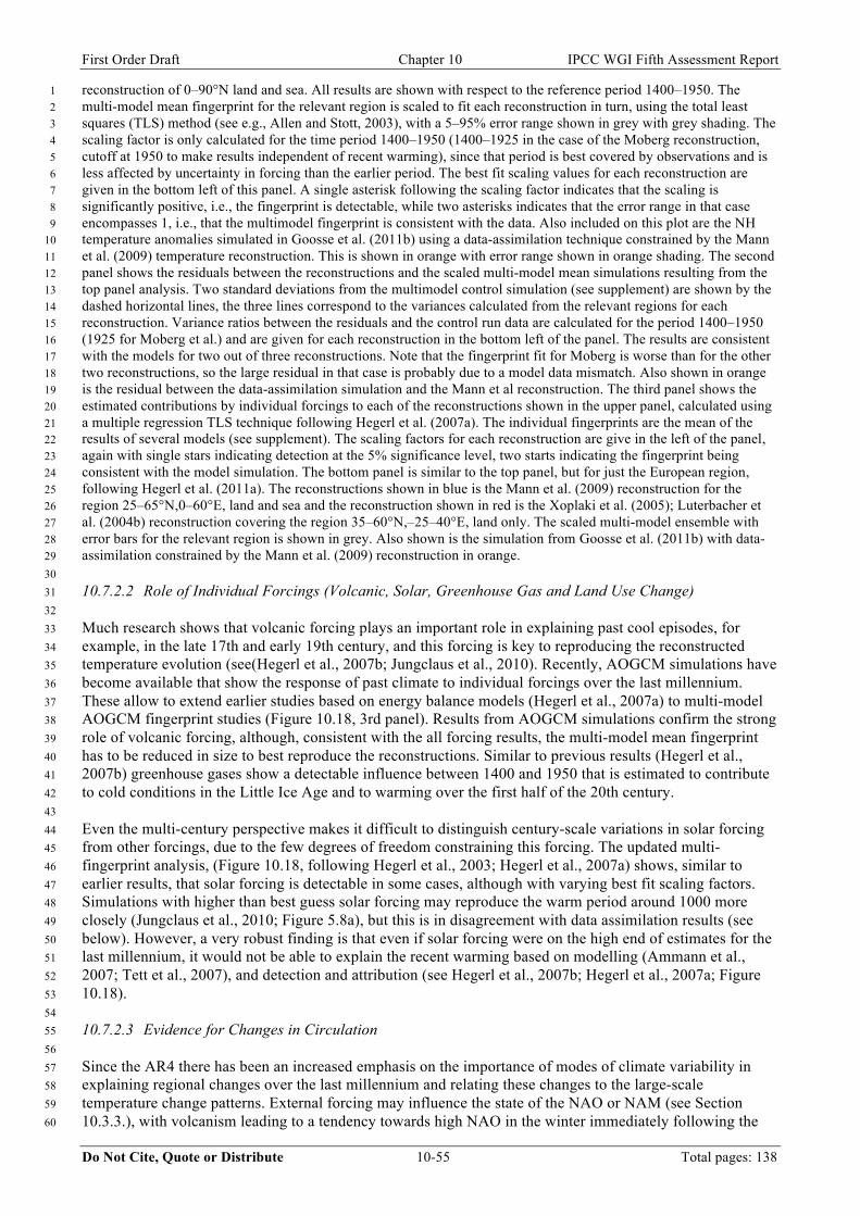
First Order Draft Chapter 10 IPCC WGI Fifth Assessment Report
Do Not Cite, Quote or Distribute 10-55 Total pages: 138
reconstruction of 0–90°N land and sea. All results are shown with respect to the reference period 1400–1950. The 1 multi-model mean fingerprint for the relevant region is scaled to fit each reconstruction in turn, using the total least 2 squares (TLS) method (see e.g., Allen and Stott, 2003), with a 5–95% error range shown in grey with grey shading. The 3 scaling factor is only calculated for the time period 1400–1950 (1400–1925 in the case of the Moberg reconstruction, 4 cutoff at 1950 to make results independent of recent warming), since that period is best covered by observations and is 5 less affected by uncertainty in forcing than the earlier period. The best fit scaling values for each reconstruction are 6 given in the bottom left of this panel. A single asterisk following the scaling factor indicates that the scaling is 7 significantly positive, i.e., the fingerprint is detectable, while two asterisks indicates that the error range in that case 8 encompasses 1, i.e., that the multimodel fingerprint is consistent with the data. Also included on this plot are the NH 9 temperature anomalies simulated in Goosse et al. (2011b) using a data-assimilation technique constrained by the Mann 10 et al. (2009) temperature reconstruction. This is shown in orange with error range shown in orange shading. The second 11 panel shows the residuals between the reconstructions and the scaled multi-model mean simulations resulting from the 12 top panel analysis. Two standard deviations from the multimodel control simulation (see supplement) are shown by the 13 dashed horizontal lines, the three lines correspond to the variances calculated from the relevant regions for each 14 reconstruction. Variance ratios between the residuals and the control run data are calculated for the period 1400–1950 15 (1925 for Moberg et al.) and are given for each reconstruction in the bottom left of the panel. The results are consistent 16 with the models for two out of three reconstructions. Note that the fingerprint fit for Moberg is worse than for the other 17 two reconstructions, so the large residual in that case is probably due to a model data mismatch. Also shown in orange 18 is the residual between the data-assimilation simulation and the Mann et al reconstruction. The third panel shows the 19 estimated contributions by individual forcings to each of the reconstructions shown in the upper panel, calculated using 20 a multiple regression TLS technique following Hegerl et al. (2007a). The individual fingerprints are the mean of the 21 results of several models (see supplement). The scaling factors for each reconstruction are give in the left of the panel, 22 again with single stars indicating detection at the 5% significance level, two starts indicating the fingerprint being 23 consistent with the model simulation. The bottom panel is similar to the top panel, but for just the European region, 24 following Hegerl et al. (2011a). The reconstructions shown in blue is the Mann et al. (2009) reconstruction for the 25 region 25–65°N,0–60°E, land and sea and the reconstruction shown in red is the Xoplaki et al. (2005); Luterbacher et 26 al. (2004b) reconstruction covering the region 35–60°N,–25–40°E, land only. The scaled multi-model ensemble with 27 error bars for the relevant region is shown in grey. Also shown is the simulation from Goosse et al. (2011b) with data-28 assimilation constrained by the Mann et al. (2009) reconstruction in orange. 29 30 10.7.2.2 Role of Individual Forcings (Volcanic, Solar, Greenhouse Gas and Land Use Change) 31 32 Much research shows that volcanic forcing plays an important role in explaining past cool episodes, for 33 example, in the late 17th and early 19th century, and this forcing is key to reproducing the reconstructed 34 temperature evolution (see(Hegerl et al., 2007b; Jungclaus et al., 2010). Recently, AOGCM simulations have 35 become available that show the response of past climate to individual forcings over the last millennium. 36 These allow to extend earlier studies based on energy balance models (Hegerl et al., 2007a) to multi-model 37 AOGCM fingerprint studies (Figure 10.18, 3rd panel). Results from AOGCM simulations confirm the strong 38 role of volcanic forcing, although, consistent with the all forcing results, the multi-model mean fingerprint 39 has to be reduced in size to best reproduce the reconstructions. Similar to previous results (Hegerl et al., 40 2007b) greenhouse gases show a detectable influence between 1400 and 1950 that is estimated to contribute 41 to cold conditions in the Little Ice Age and to warming over the first half of the 20th century. 42 43 Even the multi-century perspective makes it difficult to distinguish century-scale variations in solar forcing 44 from other forcings, due to the few degrees of freedom constraining this forcing. The updated multi-45 fingerprint analysis, (Figure 10.18, following Hegerl et al., 2003; Hegerl et al., 2007a) shows, similar to 46 earlier results, that solar forcing is detectable in some cases, although with varying best fit scaling factors. 47 Simulations with higher than best guess solar forcing may reproduce the warm period around 1000 more 48 closely (Jungclaus et al., 2010; Figure 5.8a), but this is in disagreement with data assimilation results (see 49 below). However, a very robust finding is that even if solar forcing were on the high end of estimates for the 50 last millennium, it would not be able to explain the recent warming based on modelling (Ammann et al., 51 2007; Tett et al., 2007), and detection and attribution (see Hegerl et al., 2007b; Hegerl et al., 2007a; Figure 52 10.18). 53 54 10.7.2.3 Evidence for Changes in Circulation 55 56 Since the AR4 there has been an increased emphasis on the importance of modes of climate variability in 57 explaining regional changes over the last millennium and relating these changes to the large-scale 58 temperature change patterns. External forcing may influence the state of the NAO or NAM (see Section 59 10.3.3.), with volcanism leading to a tendency towards high NAO in the winter immediately following the 60

First Order Draft Chapter 10 IPCC WGI Fifth Assessment Report
Do Not Cite, Quote or Distribute 10-56 Total pages: 138
eruption. Low solar forcing may lead to a decrease in westerlies, and an increased tendency towards 1 blocking, as evidenced by a composite analysis using reanalysis data (e.g., Woollings et al., 2010). There is 2 suggestive evidence for ENSO responding to volcanism (Adams et al., 2003; Section 5.4.3), although 3 uncertainties are large. There is also suggestive evidence for a role of circulation changes in explaining 4 patterns of climate change over the last millennium (Mann et al., 2009), Consistent with that, results from a 5 data assimilation technique (Goosse et al., 2010; Goosse et al., 2011b) suggest that atmospheric circulation 6 played a role in the medieval climate anomaly (MCA). Thus, there is suggestive evidence for a role in 7 atmospheric circulation in contributing to the warm conditions in the medieval warm period, with significant 8 uncertainties in the spatial and seasonal patterns, and in the data. While there is some agreement between 9 models and reconstructions for the MCA, these uncertainties constrain the results to medium confidence. 10 Note that comparisons between spatial patterns in models and data are inconclusive unless the probability of 11 an agreement by chance and the quantitative ability of the model to explain reconstructed changes is 12 assessed. 13 14 10.7.3 Changes of Past Regional Temperature 15 16 Several reconstructions of past regional temperature variability are available (Section 5.4.1). Luterbacher et 17 al. (2004a), (see also Xoplaki et al., 2005) reconstructed temperature variability in Europe from 1500 18 onwards for all four seasons, with the reconstructions dominated by evidence from documents throughout 19 this period and by instrumental data from the late 17th century to present. The Northern Hemispheric spatial 20 reconstruction of Mann et al. (2009) also provides a European sector reconstruction. Bengtsson et al. (2006) 21 concluded that preindustrial European climate captured in the Luterbacher reconstruction is ‘fundamentally a 22 consequence of internal fluctuations of the climate system’. This conclusion is based on the consistent 23 variability found for short timescales in an OAGCM control simulation and this reconstruction. However, 24 Hegerl et al. (2011a) analyzed 5-year averaged European seasonal temperatures and find a detectable 25 response to external forcing in summer temperatures in the period prior to 1900, and detectable signals 26 throughout the record (1500 to 1999 also 1500 to 1950) for winter and the entire record for spring . These 27 authors use a multi-model fingerprint of temperature change over time that is derived from three model 28 simulations with slightly different combinations of external forcings. Despite the forcing uncertainties, the 29 fingerprint for external forcing shows coherent time evolution between models and reconstructed 30 temperatures over the entire analysed period (both before and after 1900), and suggests that the cold winter 31 conditions in the late 17th and early 19th century and the warming between these two cold periods were 32 externally driven. The role of forcing in European temperatures is also detectable in the European sector 33 from the reconstruction by Mann et al. from 1400 onward (Mann et al., 2008; Figure 10.18). 34 35 Recent data assimilation results focusing on the European sector display both a response of European 36 temperatures to external forcing and a role of internal dynamics (Goosse et al., 2011a, see also Section 37 10.7.2.3). While both forced only and assimilated simulation closely follow the reconstructions from 1400 38 onwards, the assimilated simulations reproduce the medieval warm period more closely than the forced only 39 simulations (Goosse et al., 2011a; Figure 10.18) (see further discussion below). 40 41 The response to individual forcings is more difficult to detect and distinguish from each other in noisier 42 regional reconstructions. In the multi-fingerprint approach for European seasonal temperatures, only 43 greenhouse gas forcing was clearly detectable in winter for the period 1500–1950, although there was some 44 evidence for a role of solar forcing in summer (Hegerl et al., 2011a). An epoch analysis of years immediately 45 following volcanic eruptions shows that European summers following volcanic eruptions are significantly 46 colder than average years, while winters show a response of warming in Northern Europe and cooling in 47 Southern Europe (Hegerl et al., 2011a). However, multiple eruptions need to be combined in order to be able 48 to distinguish, particularly, the winter response from climate variability. Thus, there is medium evidence for 49 an influence by external forcing on European temperatures from 1500 onwards. 50 51 10.7.4 Causes or Contributors to Change in Specific Periods 52 53 Here two periods of particular interest are assessed, the little ice age and the Medieval climate anomaly. 54 55 10.7.4.1 The Little Ice Age 56 57

First Order Draft Chapter 10 IPCC WGI Fifth Assessment Report
Do Not Cite, Quote or Distribute 10-57 Total pages: 138
The Little Ice Age is a period of relatively cool conditions, peaking from 1550–1750 and again about 1810–1 1840 (see Chapters 5 and 9). Radiative forcing in the little ice age on long time scales includes a drop in 2 solar forcing (with uncertain amplitude), and a slight reduction in greenhouse gases concentration in the 3 atmosphere (Chapter 5). The late 17th and early 19th century was also characterised by substantial pulses of 4 volcanism, including the powerful eruption of Mount Tambora in 1815. These pulses of volcanism can lead 5 to long-term cooling in models despite the short lived nature of the forcing (see Gregory et al., 2011; Tett et 6 al., 2007 and updates thereof). The overall temperature difference between the cold periods in the late 17th 7 and early 19th century and the 20th century varies between reconstructions. Modelling studies reproduce this 8 cooling if forced with a combination of solar, volcanic, and greenhouse gas forcing (Ammann et al., 2007; 9 Jungclaus et al., 2010; Tett et al., 2007). However, it is unclear if larger solar forcing helps to explain the 10 cold conditions in the little ice age (e.g., Foukal et al., 2006), or if the Little Ice Age is reproduced better with 11 intermediate to small solar forcing (Ammann et al., 2007). Detection and attribution results are usually based 12 on longer time periods that include the LIA, and confirm a role for both volcanic and greenhouse gas forcing 13 with probably a contribution from solar forcing, (Hegerl et al., 2007a and update; Figure 10.18) and is 14 consistent with modelling studies (Goosse et al., 2010; Jungclaus et al., 2010). Both model simulations 15 (Frank et al., 2010; Jungclaus et al., 2010) and detection and attribution studies (Hegerl et al., 2007a; Figure 16 10.18) suggest that the small drop in CO2 during the little ice age may have contributed to the cool conditions 17 during the 16th and 17th century. Palastanga et al. (2011) use a data assimilation approach where the 18 HadCM3 and ECBILT-CLIO models are nudged towards a low state of the NAO, and where water hosing 19 influences the state of the Meridional overturning circulation. Results show that neither a slowdown of the 20 thermohaline circulation nor a persistently negative NAO alone can explain the reconstructed temperature 21 pattern over Europe during parts of the Little Ice Age (periods 1675–1715 and 1790–1820), consistent with 22 the results discussed above that external forcing very likely played a role in explaining the cold conditions 23 during the LIA. 24 25 10.7.4.2 The Medieval Climate Anomaly 26 27 Temperatures in the early centuries of the last millennium were substantially warmer than the so-called Little 28 Ice Age, leading to conditions similar to the ones observed during the second half of the 20th centuries at 29 many locations, and possibly even higher temperatures at some places (Chapter 5, see also Buentgen et al., 30 2011 for Europe). However, warm conditions around the early millennium occurred at different times for 31 different locations, leading to less unusual warmth for the Northern Hemisphere as a whole compared to 32 individual regions (see Briffa et al. 2002). Climatic conditions in Europe in summer were similar to the late 33 20th century, although very recent increases in summer temperatures are highly unusual (Hegerl et al., 34 2011a; Luterbacher et al., 2004b; Hegerl et al., 2011). Goosse et al. (2006) estimate that the radiative forcing 35 for the medieval warm period, particularly for European summer, was quite similar to the recent past. They 36 argue, recent aerosol cooling and land use change (through changes in albedo) during the transition from a 37 more forested stage early in the millennium to more agricultural land in the present (Ruddiman and Ellis, 38 2009) has cancelled out a substantial part of the greenhouse gas forcing. However, this result is model 39 dependent. Solar forcing estimates in the MCA are uncertain, although results suggest an overall slightly 40 elevated solar forcing (Figure 5.1). In contrast to the LIA, the elevated temperatures caused little CO2 change 41 in that period (Frank et al., 2008). Detection and attribution analyses of the entire millennium suggest that 42 small volcanic forcing and small positive solar forcing explain the estimated warmth in some, but not all 43 records during the MCA. In addition to this response to forcing, data assimilation methods(Goosse et al., 44 2011a; Goosse et al., 2011b) suggest that long-term changes in the atmospheric circulation, characterized by 45 strengthened mid-latitude westerlies in winter and northward shifts in the position of the gulfstream and 46 Kurishio current may help explain some of the remaining model and data differences (Figure 10.18). The 47 technique, however, does not allow determining if those circulation changes are purely related to the internal 48 variability of the climate or to a response of the system to some forcing not well represented in the relatively 49 simple climate model used in those experiments. Jungclaus et al. (2009) compare different reconstructions of 50 cooling between the Medieval Climate Anomaly and the Little Ice Age (Figure 10.22, see also Chapters 5 51 and 9) and find that their model can reproduce the changes between both periods within data and forcing 52 uncertainty, and that higher than present best estimate solar forcing explains the change between both 53 periods for reconstructions better. In contrast, Goose et al.’s data assimilation method does not yield 54 substantially better agreement with high solar forcing because the reconstructed spatial structure of the 55 changes during the MCA does not fit to the one of the response to solar forcing in their model. During the 56 MCA, some of the reconstructions remain warmer than the best estimates obtained by climate model, with 57

First Order Draft Chapter 10 IPCC WGI Fifth Assessment Report
Do Not Cite, Quote or Distribute 10-58 Total pages: 138
and without data assimilation, when driven by the current relatively uncertain reconstructions of the external 1 forcing. 2 3 In conclusion, models and data are not in disagreement given the substantial uncertainties that exist in the 4 data and forcing, but some reconstructions remain warmer than climate model simulations. 5 6 10.7.5 Changes in Regional Precipitation, Drought and Circulation 7 8 Reconstructions of past regional precipitation and drought (see Chapter 5) suggest substantial regional 9 droughts have occurred. For example, in western North America (Cook et al., 2007) (see Chapter 5), the past 10 droughts often exceeded droughts recorded in the 20th century. Research suggests a role of tropical Pacific 11 variability in these large droughts. Seager et al. (2008) show that if forced with SSTs reconstructed from 12 corals, a large ensemble of atmospheric model produces droughts that match mega droughts in North 13 America in the 14th and 15th century that have been recorded from tree ring data. However. this ensemble 14 failed to reproduce the wetter period between these two dry periods. The megadroughts in the ensemble are 15 associated by extended La-Nina like states. Herweijer and Seager (2008) show that dry conditions in western 16 North America in the 19th and early 20th century coincided with dry conditions in Europe, southern South 17 American and western Australia, and coincide with cool conditions of the Eastern Tropical Pacific. 18 19 10.7.6 Estimates of Unforced Internal Climate Variability 20 21 The residual variability in past climate that is not explained by changes in radiative forcing provides an 22 estimate of internal variability of the climate system that is independent from the 20th century instrumental 23 period. As the level of internal variability is the background against which forced signals are detected, an 24 estimate of internal climate variability that is largely independent of climate modelling is invaluable because 25 it is not certain whether climate models realistically generate the internal variability of the climate system on 26 long timescales. The residual variability is not completely independent of climate models, because the forced 27 signal fingerprint is diagnosed from models. However, model errors would result in incomplete removal of 28 the true forced signal which would tend to overestimate past variability and therefore provide a conservative 29 test of climate model internal variability. The 1400–1950 residual of decadal smoothed climate variability 30 that is not accounted for by the multi-regression varies strongly with reconstruction, but is, within that 31 uncertainty, consistent with the internal climate model variability from the control simulations of those 32 climate models that provided the fingerprints (see supplement). An exception is the reconstruction by 33 Moberg et al., whose variability is not as well captured by climate model fingerprints yielding larger 34 residuals (see also Hegerl et al., 2007a). 35 36 If the multi-model fingerprint, based on 1400–1950 scaling factors, is subtracted from the entire 37 reconstruction, then the residual decadal variability prior to 1400 shows fairly large excursions for some 38 reconstructions (Figure 10.18). These large excursions are consistent with model simulations not matching 39 the warm conditions in some reconstructions (Chapters 5, 9; see Section 10.7.2.1). ). One of these excursions 40 in the residual is due to the cooling associated with the volcanic eruption in 1258 being much stronger in 41 most simulations than in the reconstructions, possibly because the volcanic forcing for this eruption may 42 have been overestimated (Timmreck et al., 2009 or Mann et al., 2011). 43 44 The interdecadal and longer-term variability in large-scale temperatures in climate model simulations with 45 and without past external forcing is quite different (Jungclaus et al., 2010; Tett et al., 2007), suggesting that a 46 large fraction of temperature variance in the last millennium has been externally driven (>50% on decadal 47 and hemispheric scales (Hegerl et al., 2003; Hegerl et al., 2007a), even over the pre-instrumental period. This 48 is in agreement with detection and attribution studies (Hegerl et al., 2007a; Jungclaus et al., 2010). While the 49 inter-decadal temperature variability is similar to that in climate model control simulations (given uncertainty 50 in the reconstruction and removal of the forced component), the updated result (Figure 10.18) raises the 51 possibility that variability in some climate models may be less than that recorded. 52 53 10.7.7 Summary: Lessons from the Past 54 55 Reconstructions and long records of past climate support a significant role of external forcing on climate 56 variability and change, particularly on hemispheric scales. Climate model simulations forced with realistic 57

First Order Draft Chapter 10 IPCC WGI Fifth Assessment Report
Do Not Cite, Quote or Distribute 10-59 Total pages: 138
estimates of past natural and anthropogenic forcings can reproduce climate variability back to 1400, and 1 reproduce periods back to the 8th century within wider uncertainty levels. Detection and attribution studies 2 show that this agreement is not spurious, and that the time evolution of forcings points at volcanic forcing 3 and CO2 forcing, as well as possible solar forcing being important to explain past changes in Northern 4 Hemispheric temperatures. Results from data assimilation runs and data model comparisons indicate that 5 changes in modes of variability may have contributed to climate anomalies, e.g., the so-called medieval 6 warm period and the little ice age. The role of external forcing extends to regional records, for example, 7 European seasonal temperatures, where the response to all forcings combined is detected over the period 8 1500 to 1900 in summer, and 1500 to 1950 in winter. The reconstructions do not suggest that climate models 9 underestimate internal variability of temperature on large spatial scales by a significant amount. Changes in 10 circulation may have shaped regional climate variability, and have contributed, for example, to the warm 11 conditions early in the millennium. In summary, the evidence across a wide range of studies support and 12 strengthen our confidence in the conclusion that external forcing combined with internal variability as 13 estimated by climate models are very likely to have contributed to Northern Hemispheric temperature 14 variability from 1400 to 1950. Results for the entire millennium are less certain, largely due to increased 15 uncertainties in reconstructions of forcing and temperature change. 16 17 10.8 Whole System Attribution 18 19 The evidence accumulated from widespread anthropogenic changes detected in aspects of the climate 20 system, and documented in the preceding sections, including in near surface temperature (Section 10.3.1.1), 21 free atmosphere temperature (Section 10.3.1.2), atmospheric moisture content (Section 10.3.2), precipitation 22 over land (Section 10.3.2), ocean heat content (Section 10.4.1), ocean salinity (Section 10.4.2), and Arctic 23 sea ice (10.5) as well as in aspects of climate extremes (Section 10.6) strengthens the conclusion that human 24 influence has played the dominant role in observed warming over the past several decades. However the 25 approach of the chapter so far has been to examine each aspect of the climate system – the atmosphere and 26 surface, the ocean, the cryosphere, aspects of extremes – separately. In this section we look across the whole 27 climate system to assess to what extent a consistent picture emerges across sub-systems and across climate 28 variables. 29 30 10.8.1 Multivariable Studies 31 32 There have been relatively few applications of multi-variable detection and attribution studies in the 33 literature. A combined analysis of near-surface temperature from weather stations and free atmosphere 34 temperatures from radiosondes detected an anthropogenic influence on the joint changes in temperatures near 35 the surface and aloft (Jones et al., 2003). In a Bayesian application of detection and attribution (Schnur and 36 Hasselmann, 2005) combined surface temperature, diurnal temperature range and precipitation into a single 37 analysis and showed strong net evidence for detection of anthropogenic forcings despite low likelihood ratios 38 for diurnal temperature range and precipitation on their own. Barnett et al.(Barnett et al., 2008) applied a 39 multi-variable approach in analysing changes in the hydrology of the Western United States (see also Section 40 10.3). They constructed a multi-variable fingerprint, consisting of snow pack (measured as snow water 41 equivalent), the timing of runoff into the major rivers in the region, and average January to March daily 42 minimum temperature over the region. Observed changes were compared with the output of a regional 43 hydrologic model forced by the PCM and MIROC climate models (Figure 10.19). They derived a multi-44 variable fingerprint of anthropogenic changes from the two climate models and found that the observations, 45 when projected onto this fingerprint, show a positive signal strength consistent with the climate model 46 simulations. This observed signal falls outside the range expected from internal variability as estimated from 47 1,600 years of downscaled climate model data. The expected response to solar and natural forcing combined 48 estimated from the PCM model has a signal with the opposite sign to that observed. They conclude that there 49 is a detectable and attributable signature of human effects on the hydrology of this region with simulated 50 trends in response to human influence in their diagnostic having an amplitude with a best estimate of 51 between 30% and 60% of the observed trend, depending on the model and downscaling method applied. 52 53 [INSERT FIGURE 10.19 HERE] 54 Figure 10.19: Observed time series of selected variables (expressed as unit normal deviates) used in the multivariate 55 detection and attribution analysis. Taken in isolation, seven of nine SWE/P, seven of nine JFM Tmin, and one of the 56 three river flow variables have statistically significant trends (Barnett et al., 2008). 57

First Order Draft Chapter 10 IPCC WGI Fifth Assessment Report
Do Not Cite, Quote or Distribute 10-60 Total pages: 138
1 While their analysis shows clearly that the three variables are changing coherently in a systematic fashion, 2 how much additional information is provided by snow mass and timing of river flows in addition to 3 temperature Barnett et al. (2008) examine signal to noise ratios and find that the signal to noise ratio of their 4 multi-variable fingerprint is higher than for each of the individual three components, confirming that the 5 multi-variable fingerprint has higher detectability, although it should be noted that the two hydrological 6 components studied are closely related to temperature. 7 8 The potential for a multi-variable analysis to have greater power to discriminate between forced changes and 9 internal variability was also demonstrated by Stott and Jones (2009), in this case for a different combination 10 of climate variables. They showed that a multi-variable fingerprint consisting of the responses of global 11 mean temperature and sub-tropical Atlantic salinity has a higher signal to noise than the fingerprints of each 12 variable separately. They found reduced detection times as a result of low correlations between the two 13 variables in the control simulation although the detection result depends on the ability of the models to 14 represent the co-variability of the variables concerned. Multi-variable attribution studies potentially provide a 15 stronger test of climate models than single variable attribution studies although there can be sensitivity to 16 weighting of different components of the multi-variable fingerprint, when several variables are convolved 17 into one analysis, it is not necessarily clear where inconsistencies come from, and the inclusion of additional 18 variables in multi-variable studies may add little extra information since non-informative components cannot 19 increase power. 20 21 Further insights can be gained from considering a synthesis of evidence across the climate system. This is the 22 subject of the next subsection. 23 24 10.8.2 Earth System Analysis 25 26 To build robust interpretations of the observed climate changes in terms of the causes we rely on this meta 27 analysis of a suite of studies across all of the common elements of the of the climate system. The 28 instrumental records associated with each element of the climate system are generally independent, and 29 consequent joint interpretations across observations from the main components of the climate system 30 increases the confidence to even higher levels than any single study. Similarly, using models of the climate 31 system, and demanding that they replicate the response of the different forcings (within internal variability) 32 across a wider suite of climate indicators also build confidence in the CMIP3 and CMIP5 models, and 33 connects more powerfully observations with theory. 34 35 Table 10.1 illustrates a suite of detection and attribution results across these elements of the climate system, 36 for global variables (like surface temperature), across the different components that cover the instrumental 37 record and the records derived from paleo-reconstructions on a range of time scales ranging from extreme 38 precipitation events to millennium timescales. 39 40 The surface of the earth, the upper oceans (ocean heat content and thermal expansion), the troposphere, and 41 the temperature gradient between the troposphere and stratosphere all have anthropogenic forced signals that 42 exceed internal variability of the climate system. Indeed to successfully describe the observed global trends 43 in these three components since the1960 and 1970's contributions from both anthropogenic forcing and 44 natural forcings (ie volcanic eruptions and solar) are required (results 1,2,3,4 and 9,10, and 5,7). This is 45 consistent with anthropogenic forcing warming the surface of the earth, troposphere and oceans more than 46 observed, and that the three large eruptions since the 1960's have cooled these components, and these two 47 causes give the observed response (see also Figures 10.1, 10.4, 10.5, 10.6 and 10.15). This is an important 48 because both sources of forcing are required to understand underlying causes of warming of the earth system. 49 The many studies that support this attribution to anthropogenic forcing of the climate range in confidence 50 level from very likely for the troposphere to virtually certain for the long term trends in ocean heat content. 51 52 Water in the free atmosphere is expected to increasing, and at local scales expected to increase from 53 Clausius-Claperyon equation as a consequence of warming at 7% K–1. Atmospheric circulation controls 54 global distribution of rain and evaporation. Simulations show that greenhouse gases increase moisture 55 transport and amplify these global patterns or rain and evaporation, although some aspects of this rain are 56 affected by tropospheric aerosols. The patterns of rain and evaporation are quite distinct from the patterns of 57

First Order Draft Chapter 10 IPCC WGI Fifth Assessment Report
Do Not Cite, Quote or Distribute 10-61 Total pages: 138
warming. The observations show that water is increasing in the free atmosphere (16, medium confidence) 1 evidence, that precipitation is increasing in wet areas and reducing in dry areas (13,14, medium confidence) 2 in the Northern Hemisphere, and the global patterns of ocean salinity at the surface (and at depth) also 3 confirms this tendency (since 1960, 11, likely) for the wet regions becoming wetter and the dry regions 4 becoming dryer. These results together give a global coverage of the earth's surface. 5 6 Warming of the atmosphere and the oceans can affect the cryosphere, and in the case of snow and sea-ice 7 lead to positive feedbacks that amplify the warming response in the atmosphere and oceans. Mountain 8 Glaciers detected to have a anthropogenic influence (17, likely), Greenland ice sheet is melting at the edges 9 and tending accumulate snow in the higher elevations consistent with greenhouse gas warming and the 10 surface mass balance is significantly negative (18, likely). Our level scientific understanding is too low to 11 provide a satisfactory quantifiable explanation of the observed mass loss of Antarctic (18). Sea ice in the 12 Arctic is decreasing rapidly and the changes now exceeds the internal variability (19, likely) while Antarctic 13 sea ice extent is growing but within the envelope internal variability of climate models (20, medium 14 confidence). The warming is likely to be reducing the amount of snow cover and permafrost (21). 15 16 Some aspects of the atmospheric circulation have changed, such as widening of the Hadley Cell (24, medium 17 confidence), while some aspects have remained the same with no detectable trend such as the North Atlantic 18 Oscillation (22, medium), while the Southern Annular Mode has a detectable strengthening (23, likely). The 19 warming is also affecting temperature on continental scales, with human influences detected in mean 20 temperature on all continents (medium confidence), including Antarctica (low confidence). On millenium 21 time scales anthropogenic forcing and volcanic eruptions are detected in Europe in some seasons (29, 22 medium confidence). By contrast it is likely that extremes in temperature has been detected at some sub-23 continental scales (30) and that the probability of heatwaves has risen (31, likely). 24 25 10.9 Implications for Climate System Properties and Projections 26 27 Detection and Attribution results provide information on the causes of past climate change and also provide 28 estimates of the magnitude of the climate response to external forcing. These estimates of the response can 29 be used to predict future changes, based on projections of the same forcing, for example, future increases in 30 greenhouse gases. The value and strength of the constraint on future changes depends on how relevant 31 observable climate changes are for the predicted response, and on the signal-to-noise ratios of the change 32 considered. Transient climate response is a measure of the magnitude of transient warming while the system 33 is not in equilibrium, and is particularly relevant for near-term temperature changes (Section 10.9.1; Annex 34 1; Glossary). It is also tighter constrained by the observed, transient warming than the equilibrium sensitivity 35 (see, for example, (Baker and Roe, 2009; Frame et al., 2005). Comparisons of simulated and observed 36 precipitation changes provide evidence that climate models could underestimate recent changes in mean and 37 intense precipitation, suggesting that they may also underestimate projected future changes (Section 10.9.2). 38 The Equilibrium Climate Sensitivity (ECS; Section 10.9.4) is relevant to determining the CO2 concentration 39 levels that keep global warming below particular thresholds in the long term, under equilibration or long-40 term climate response (see, e.g., Solomon et al., 2009). Constraints on estimates of longer-term climate 41 change and equilibrium climate change from recent warming hinge on the rate at which the ocean has taken 42 up heat, and for both transient and equilibrium changes. The amount of recent warming prevented by aerosol 43 forcing is relevant. Therefore, attempts to estimate climate sensitivity (transient or equilibrium) often also 44 estimate the total aerosol forcing and the rate of ocean heat uptake (Section 10.9.4). 45 46 The AR4 had for the first time a detailed discussion on estimating these quantities relevant for projections, 47 including equilibrium climate sensitivity and transient climate response, and included an appendix with the 48 relevant methods. We build on the AR4 here, repeating some information and discussion where necessary to 49 provide context. 50 51 10.9.1 Transient Climate Response 52 53 The AR4 discussed for the first time estimates of the transient climate response, or TCR, which was 54 originally defined as the warming at the time of CO2 doubling (i.e., after 70 years) in a 1% yr–1 increasing 55 CO2 experiment (see Hegerl et al., 2007b). Like ECS, TCR can also be thought of (Frame et al., 2006; Held 56 et al., 2010) as a generic property of the climate system that determines the transient response to any gradual 57

First Order Draft Chapter 10 IPCC WGI Fifth Assessment Report
Do Not Cite, Quote or Distribute 10-62 Total pages: 138
increase in radiative forcing taking place over a similar timescale. Held et al. (2010) use the simple two-box 1 model of Gregory et al. (2000) in which TCR is determined by the heat capacity of the ocean mixed layer, a 2 radiative damping term corresponding to the ‘fast’ climate sensitivity, and the rate of heat uptake by the deep 3 ocean. To the extent that deep ocean heat uptake is simply proportional to the temperature difference 4 between the mixed layer and deep ocean, then the deep ocean heat exchange affects the surface temperature 5 response as if it were an enhanced radiative damping: hence the difficulty of placing an upper bound on 6 climate sensitivity from the observed surface warming alone (Forest et al., 2002; Frame et al., 2005). Heating 7 of the deep ocean introduces a slow, or ‘recalcitrant’, component of the response. Held et al. (2010) noted 8 that this recalcitrant response could not be reversed for many decades even if it were possible to return 9 radiative forcing to pre-industrial values. To the extent that the fast response is linear, Held’s ‘transient 10 climate sensitivity ‘(TCS) as well as TCR is independent of the actual percent-per-year rate of CO2 increase, 11 and hence can be estimated from the response to any transient forcing operating over a similar timescale. 12 This is similar in motivation to the ‘normalised TCR’ (NTCR), defined by Frame et al. (2006) as the rate of 13 warming in degrees per year divided by the fractional rate of CO2 increase per year over a 70-year period: 14 both TCS and NTCR were introduced to avoid the apparent scenario-dependence of the traditional definition 15 of TCR. Since, however, both are just multiples of TCR itself (TCS=TCR/F2x; NTCR=TCR/0.7), it is not 16 necessary to introduce new notation, and TCR as well as ECS describe general emergent properties of a 17 climate model or the climate system itself rather than outcomes of specific climate model experiments. Since 18 TCR focuses on the short term response, constraining it is a key step in constraining future global 19 temperature change under scenarios where forcing continues to increase, or peak or finally stabilize (Frame 20 et al., 2006). After stabilisation, the Equilibrium climate sensitivity becomes the relevant climate system 21 property. The AR4 concluded that, based on observational constraints, the TCR is very likely to be larger 22 than 1°C and very unlikely to be greater than 3.5°C (Hegerl et al., 2007b). This supported the overall 23 assessment that the transient climate response is very unlikely greater than 3°C and very likely greater than 24 1°C (Meehl et al., 2007a). Meanwhile, several new estimates of the TCR are now available: 25 26 The recently observed climate change provides opportunities to estimate the TCR (Allen et al., 2000; Hegerl 27 et al., 2007b) from recent climate change. For scaling factors derived from fingerprint detection and 28 attribution (see Section 10.2) express how model derived fingerprints for the response to greenhouse gases 29 and aerosols need to be scaled to match the observations over the historical period. These ranges may be 30 used to provide probabilistic projections of the future response to these forcings (Allen et al., 2000; 31 Kettleborough et al., 2007; Meehl et al., 2007b; Stott and Kettleborough, 2002; Stott and Forest, 2007; Stott 32 et al., 2008a; Stott et al., 2006b). Allen et al. (2000) and Kettleborough et al. (2007) demonstrate a near 33 linear relationship for a wide range of parameters between 20th century warming and warming by the mid-34 21st century in Energy Balance Models, thus justifying this approach for scaling future responses to arrive at 35 observationally-constrained projections of 21st century warming. Projections based on scaling factors from 36 detection and attribution (Stott et al., 2006b) were used in the AR4 (Meehl et al., 2007b), among other 37 inputs, for providing probabilistic ranges of future global temperature change. Stott et al. (2008a) 38 demonstrate that optimal detection analysis of 20th century temperature changes, using HadCM3, are able to 39 exclude very high and very low temperature responses to aerosols, or equivalently aerosol forcings. 40 Consequently, projected 21st century warming may be more closely constained than if the full range of 41 aerosol forcings is used(Andreae et al., 2005). Stott and Forest (2007) demonstrate that projections obtained 42 from such an approach are similar to those obtained by constraining energy balance model (EBM) 43 parameters from observations. Stott et al. (2011), using HadGEM2-ES, and Gillett et al. (2011a), using 44 CanESM2, both show that the inclusion of observations between 2000 and 2010 in such an analysis 45 substantially reduces the uncertainties in projected warming in the 21st century, and tends to constrain the 46 maximum projected warming to below that projected using data to 2000 only. Such an improvement in 47 observational constraints through the use of more observational data is consistent with prior expectations of 48 how additional data will narrow uncertainties (Stott and Kettleborough, 2002). 49 50 TCR estimates have been derived using a variety of methods. Knutti and Tomassini (2008) derive a 51 probability density function shifted slightly towards lower values with a 5–95% percent range of 1.11–2.34 52 K. Using a single model and observations from 1851 to 2010 Gillett et al. (2011a) derive a 5–95% range of 53 1.3–1.8 K and using a single model, but multiple sets of observations and analysis periods ending in 2010 54 and beginning in 1910 or earlier, Stott et al. (2011) derive 5–95% ranges that were generally between 1 K 55 and 3 K. Both Stott et al. (2011) and Gillett et al. (2011a) find that the inclusion of data between 2000 and 56 2010 helps to constrain the upper bound of TCR. Gillett et al. (2011a) find that the inclusion of data prior to 57

First Order Draft Chapter 10 IPCC WGI Fifth Assessment Report
Do Not Cite, Quote or Distribute 10-63 Total pages: 138
1900 also helps to constrain TCR, though Stott et al. (2011) do not find such sensitivity, perhaps due to 1 relatively low internal variability on timescales longer than 100 years in the model used by Gillett et al. 2 (2011a).Three estimates of TCR estimated in this way are shown in Fig 10.20, using greenhouse gas scaling 3 factors calculated from the HadGEM2, CNRM and CanESM2 models and from the weighted multi-model 4 mean shown in Figure 10.4. (Libardoni and Forest, 2011) estimate the transient climate response along with 5 other climate system parameters (see below) from a range of 20th century surface temperature datasets as 6 well as atmospheric and ocean temperatures and estimate a 5–95% range of TCR of 0.9 to 2.4 K. Several of 7 the estimates of TCR cited by Hegerl et al. (2007b) used estimates of 20th century radiative forcing due to 8 well-mixed greenhouse gases and these studies may have underestimated the efficacies of non-CO2 gases 9 relative to the estimates in Forster et al. (2007). Since the observationally constrained estimates of TCR are 10 based on the ratio between past attributable warming and past forcing, this could account for a high bias in 11 some of the inputs used for the AR4 estimate. Figure 10.20 provides a synthesis of observationally 12 constrained estimates of TCR. 13 14 Held et al. (2010) show that their two-box model, distinguishing the fast and recalcitrant responses, fits both 15 historical simulations and instantaneous doubled CO2 simulations of the GFDL coupled model CM2.1. In the 16 instantaneous simulations the fast response has a relaxation time of 3–5 years, and where the historical 17 simulation is almost completely described by this fast component of warming. Padilla et al. (2011) use this 18 simple model to derive an observationally-constrained estimate of the TCR of 1.3–2.6 K, similar to other 19 recent estimates. A recent study bases an estimate of TCR on the response to the 11-year solar cycle as 20 estimated from observations and reanalysis data, using discriminant analysis and find a relatively high 21 estimate (>2.5 to 3.6K, Camp and Tung, 2007). However, this estimate may be affected by different 22 mechanisms by which solar forcing across wavelengths affects climate, and despite attempts to avoid 23 aliasing the response to other forcings in the 20th century, the estimate may be influenced by it and by 24 internal climate variability (see discussion in North and Stevens, 1998). 25 26 Based on this evidence, including new evidence from new 21st century observations that were not yet 27 available to AR4, we conclude that TCR is very likely to be larger than 1°C and very unlikely to be greater 28 than 3°C. This range for TCR is smaller than given at the time of AR4, due to the stronger observational 29 constraints and the wider range of studies now available. 30 31 10.9.2 Magnitude of Precipitation Response 32 33 As discussed in Section 10.3.2.3, since the publication of the AR4 anthropogenic influence on precipitation 34 has been detected globally (Zhang et al., 2007b) and over the Arctic (Min et al., 2008a), but the detected 35 changes are larger than simulated by the multimodel mean according to the scaling factors (Noake et al., 36 2011) find that the scaling factors reduce to best estimates around 1-3 when focusing on percent changes of 37 climatological precipitation and accounting for observational uncertainty, which suggests that some of the 38 underestimate in models may be due to differences in scales resolved by model data and point observations. 39 Underestimates by models of the observed precipitation response have also been observed in the response to 40 natural forcings (Gillett et al., 2004) and anthropogenic response in Arctic land precipitation Min et al. 41 (2008a), see also Section 10.6.1.2). Min et al. (2011) find a detectable anthropogenic response in two 42 measures of precipitation extremes over the Northern Hemisphere, with a best-estimate regression coefficient 43 of 2–3 but an uncertainty range that includes one. An underestimation of changes in extreme precipitation in 44 models with prescribed SSTs has also been found in the tropics (Allan and Soden, 2008; Allan et al., 2010). 45 46 There are further indications that models may underestimate the response in the hydrological cycle: Wentz et 47 al. (2007) find that ocean-mean precipitation in SSM/I data shows an increase per unit changes in 48 temperature (hydrological sensitivity) of close to 7% K–1 over the period 1987–2006, which is larger than the 49 1–3% K–1 predicted by climate models. Other studies find that amplitude of moistening of the wet regions of 50 the tropics and drying in the dry regions is underestimated in atmospheric models forced with observed SST 51 (Allan and Soden, 2007; Allan et al., 2010). Liepert et al. (2009) find that this discrepancy may be 52 explainable by internal variability, and that the simulated hydrological sensitivity is higher for aerosol 53 forcing than it is for greenhouse gases, consistent with earlier studies arguing that precipitation is more 54 sensitive to shortwave forcings than longwave forcing (see discussion in Allen and Ingram, 2001, (Hegerl et 55 al., 2007b). This means that the apparent hydrological sensitivity will depend on the relative size of changes 56 in aerosol and GHG forcing, and that the hydrological sensitivity calculated for a period in the past in which 57

First Order Draft Chapter 10 IPCC WGI Fifth Assessment Report
Do Not Cite, Quote or Distribute 10-64 Total pages: 138
greenhouse gas and aerosol forcings were both increasing may be smaller than that for a future period where 1 aerosol forcing is decreasing while GHG forcing continues to increase. Liepert and Previdi (2009) do not 2 find a systematic difference between median simulated hydrological sensitivity in the 20th and 21st 3 centuries, based on an analysis of trends in overlapping 20-year periods, but their analysis includes a number 4 of periods in the 20th century with near-zero or negative 20-year temperature trends which would tend to be 5 associated with large positive hydrological sensitivity. This also implies that scaling the projected future 6 changes in precipitation by a regression coefficient of the observed to simulated combined anthropogenic 7 response during the 20th century would only be a valid approach if the simulated precipitation responses to 8 greenhouse gases and sulphate aerosol are under- or overestimated by the same factor. So far regression 9 coefficients for these two forcings have not been separately evaluated from observations. 10 11 To date, no studies have used attribution results for precipitation to scale projected future changes, as has 12 been done for temperature (Section 10.9.1). Nonetheless, as discussed above, there is some evidence that 13 projected future changes in mean and extreme precipitation may be underestimated by multi-model mean 14 projected changes, although there is uncertainty in observations, a lack of clarity in the role of individual 15 forcings and oceanic salinity indicates consistency between models and observations in inferred freshwater 16 forcing at the surface (Durack et al., 2011a (submitted)). 17 18 10.9.3 Constraints on Long Term Climate Change and the Equilibrium Climate Sensitivity 19 20 The equilibrium climate sensitivity (ECS) is defined as the warming in response to a sustained doubling of 21 carbon dioxide in the atmosphere relative to preindustrial levels (see AR4). The ECS cannot be immediately 22 deduced from transient warming, since the role of ocean heat uptake has to be taken into account when 23 translating attributable greenhouse warming to an estimate of the ECS (see Frame et al., 2005; Hegerl et al., 24 2007b). Nevertheless, detection and attribution results have implications for estimates of the ECS, and 25 estimating the ECS requires the same paradigm of a comparison of observed change with model results 26 given uncertainty in model, data, and internal variability. 27 28 The equilibrium to which the ECS refers to is generally assumed to be an equilibrium involving the ocean-29 atmosphere system, which does not include long-term melting of ice sheets and ice caps (see Chapter 12, 30 Section 12.5.3). The latter would lead to continued warming for a longer time before a warmer equilibrium is 31 reached (Hansen et al., 2005a). Estimates of climate sensitivity can be based on estimating, with 32 uncertainties, past warming per unit forcing changing, and then adapting this sensitivity parameter by 33 multiplying it with the forcing associated with CO2 doubling, or by fitting simple energy balance models to 34 the observed temperature evolution. However, such simple energy balance calculations introduce substantial 35 uncertainties: for example, they might assume a single response timescale rather than the multiple response 36 timescales that are observed, and cannot account for nonlinearities in the climate system that lead to changes 37 in feedbacks for different forcings, such as, for example, the Last Glacial Maximum (see Hargreaves et al., 38 2007; Yoshimori et al., 2009). Therefore, most of this section is based on estimates that use climate model 39 ensembles with varying parameters yielding varying ECS, and evaluate the ability of these models to 40 reproduce a particular observed change. From this, the probability of the different model versions being 41 correct is inferred in order to estimate a probability density function (pdf) for the ECS. As discussed in the 42 AR4, such estimates are inherently based on Bayesian statistics and therefore, even if it is not explicitly 43 obvious, involve using prior information or prior beliefs. This prior information shapes the sampling 44 distribution of the models (Annan and Hargreaves, 2011; Frame et al., 2005; Hegerl et al., 2007b) and since 45 the constraints by data for transient warming is fairly weak, results are sensitive to use of priors (Sanso and 46 Forest, 2009). Analyses that make a more complete effort to estimate all uncertainties affecting the model-47 data comparison lead to more trustworthy results, but are often more uncertain than methods that apply more 48 assumptions (Knutti and Hegerl, 2008). 49 50 The detection and attribution chapter in AR4 (Hegerl et al., 2007b) concluded that ‘Estimates based on 51 observational constraints indicate that it is very likely that the equilibrium climate sensitivity is larger than 52 1.5°C with a most likely value between 2°C and 3°C’ supporting the overall assessment that the ‘likely’ 53 range of ECS is 2–4.5, but that higher values cannot be excluded, and that ECS is very likely to be larger 54 than 1.5°C’(Meehl et al., 2007b).This section re-assesses the evidence on ECS from observed changes. 55 Readers should refer to the AR4 for a more complete explanation of methods and theory. 56 57

First Order Draft Chapter 10 IPCC WGI Fifth Assessment Report
Do Not Cite, Quote or Distribute 10-65 Total pages: 138
10.9.3.1 Estimates from Recent Surface Temperature Change 1 2 Many estimates of the equilibrium climate sensitivity in AR4 were based on climate change that has been 3 observed over the instrumental period (Hegerl et al., 2007b), and their ranges are given in Figure 10.20 for 4 comparison with new estimates. The distribution of ECS estimates are wide and cannot exclude high 5 sensitivities, particularly when the forcing uncertainty, including that by aerosols, is considered fully 6 (Tanaka et al., 2009). The main reason for wide estimates of ECS based on 20th century warming is that 7 based on surface temperature alone, and even based on surface temperature data combined with ocean 8 warming data the possibility cannot be excluded, within data uncertainties, that a strong aerosol forcing or a 9 large ocean heat uptake might have masked a strong greenhouse warming (see, e.g., Stern, 2006; Forest et 10 al., 2002; Frame et al., 2006; Hannart et al., 2009; Roe and Baker, 2007; Urban and Keller, 2009). This is 11 consistent with the finding that a set of models with a larger range of ECS and aerosol forcing than the 12 ranges spanned in the CMIP3 ensemble could be consistent with the observed warming (Kiehl, 2007). 13 Application of fingerprint methods to isolate the greenhouse gas attributable warming can yield substantially 14 more information, and with it tighter estimates (Hegerl et al., 2007b; Stott and Kettleborough, 2002; Frame 15 et al., 2005), than results based on global mean diagnostics (Tanaka et al., 2009). This is not appreciated in a 16 recent estimate of the uncertainty in climate sensitivity and aerosol forcing combined (Schwartz et al., 2010) 17 that suggests that based on global temperature alone, aerosol forcing would need to be constrained in order to 18 enable estimates of future warming. 19 20 Since the AR4, Forest et al. (2008) have updated their study using a newer version of the MIT model used in 21 earlier studies (see Figure 10.24), and have extended the result to using 5 different surface temperature 22 datasets in order to account for processing uncertainty in the surface temperature record (Libardoni and 23 Forest, 2011). The overarching 5–95% range of effective climate sensitivity widens from 2–5 K from (Forest 24 et al., 2008) to 1.2–5.3 K if all five datasets are used, and constraints on ocean diffusivity become very weak. 25 The authors point out that this result is affected by uncertainty in how the ECS relates to the longterm 26 response to doubling of CO2 (see discussion above). Also, uncertainties may increase if further estimates of 27 forcing uncertainty, e.g., due to natural forcings, are considered (Forest et al., 2006). Sanso and Forest (2009) 28 further show, using a Bayesian approach, that the prior has strong influences on the resulting estimate of 29 ECS. Huber and Knutti (2011) similarly analyze the observed record from 1850 on for surface temperature, 30 and ocean heat content since the middle of the 20th century, and find that particularly the choice of ocean 31 data causes uncertainty. They find a 5–95% range of 1.8–6.6°C and a TCR range of 1.3–2.3°C. 32 33 In summary, recent work on instrumental temperature change yields very low and high sensitivity unlikely, 34 but cannot provide a tight constraint on ECS. 35 36 10.9.3.2 Estimates Based on Top-of the Atmosphere (TOA) Radiative Balance 37 38 Since the satellite era, measurements are available of the energy budget of the planet, which can directly 39 quantify the radiative imbalance of incoming shortwave and outgoing longwave radiation. Using a simple 40
energy balance relationship of the form (Murphy et al., 2009), where N is the net energy 41
flow towards the Earth (which will decay to zero as the equilibrium is reached), F is the net forcing, λ is the 42
climate feedback parameter and ε is an uncertainty term due to noise and measurement uncertainty, the 43
measurements could in theory provide tight constraints on the sensitivity of the atmosphere by providing 44 very direct estimates of the climate feedback parameter as the regression coefficient of radiative forcing 45 against global mean temperature, which is inversely proportional to the ECS (see AR4; Forster and Gregory, 46 2006). An estimate is shown in Figure 10.20, both applying a uniform prior in ECS and a prior that is 47 uniform in feedbacks (Hegerl et al., 2007b). However, the trend in shortwave outgoing radiation and with it 48 net radiation budget is affected by uncertainties in measurements, (Harries and Belotti, 2010). Lin et al. 49 (2010) estimate a climate feedback coefficient ranging from –1.3 to –1.0 W/(m2 K), which uses a model-50 estimated single valule of TOA imbalance from (Hansen et al., 2005a) and is hence uncertain. Lindzen and 51 Choi (2009) used data from the radiative budget and simple energy balance models over the tropics to 52 investigate if the feedbacks shown in climate models are realistic. The authors claim based on their 53 comparison, climate models overestimate the outgoing shortwave radiation compared to ERBE data, leading 54 to an overall mis-estimation of the radiative budget. However, the ERBE decrease in outgoing shortwave 55 radiation is highly uncertain as discussed in Harries and Belotti (2010). Also, the result of Lindzen and Choi 56 (2009) is derived from temperatures of the tropics (20°N–20°S) only, which tends to lead to substantially 57

First Order Draft Chapter 10 IPCC WGI Fifth Assessment Report
Do Not Cite, Quote or Distribute 10-66 Total pages: 138
underestimated uncertainties of global balances (Chung et al., 2010; Trenberth et al., 2010), as high latitude 1 feedbacks can be substantial (Murphy et al., 2009). Spencer and Braswell (2008) suggest a systematic bias in 2 analysis methods for feedbacks, which would bias estimates of feedback to low values, and estimates of 3 sensitivity to high values. However, Murphy and Forster (2010) show that Spencer and Braswell’s estimate 4 relaxes to values more consistent with climate models if using more realistic assumptions (e.g., realistic 5 ocean effective mixed layer depth), more realistic OLR error estimates and more comparable values for 6 models and observations (Murphy and Forster, 2010). Murphy et al. (2009) point out that estimates of λ are 7
not suitable to estimate the ECS, since multiple timescales are involved in feedbacks that contribute to 8 climate sensitivity (Knutti and Hegerl, 2008); Lin et al., 2010) and thus a simple relationship as above will 9 yield misleading and non-robust estimates for ECS as long as N is non-zero. In conclusion, some recent 10 estimates of high feedback/low sensitivities based on aspects of the observed radiative budget appear not to 11 be robust to data and method uncertainties. Consequently present TOA radiation budgets appear consistent 12 with other estimates of climate sensitivity but are unable to further robustly constrain these sensitivity 13 estimates (Bender, 2008). 14 15 10.9.3.3 Estimates Based on Response to Natural Forcing or Internal Variability 16 17 Some recent analyses have used the well observed forcing and response to major volcanic eruptions during 18 the 20th century. The constraint is fairly weak since the peak response to short-term volcanic forcing has a 19 nonlinear dependence on equilibrium sensitivity, yielding only slightly enhanced peak cooling for higher 20 values of S (Boer et al., 2007; Wigley et al., 2005). Nevertheless, models with climate sensitivity in the range 21 of 1.5 to 4.5 degrees generally perform well in simulating individual volcanic eruptions (Hegerl et al., 22 2007b). Recently, Bender at al. (2010) re-evaluated the constraint and find that there is a close relationship in 23 9 out of 10 AR4 models between the shortwave TOA imbalance, the simulated response to the eruption of 24 Mount Pinatubo and the ECS. Applying the constraint from observations suggests a range of ECS of 1.7–4.1 25 K, which, however, is subject to observational uncertainty, uncertainty due to internal climate variability, and 26 derived from only a limited sample of models. (Tung et al., 2008) estimate an ECS of >3.8°C based on the 27 estimated TCR in response to solar cycle, which however, is highly uncertain (see above), also due to the ad 28 hoc link of ECS to TRC. (Kirk-Davidoff, 2009; Schwartz, 2007) tried to relate the ECS to the strength of 29 natural variability using the fluctuation dissipation theorem but studies suggest that the observations are too 30 short to support a well constrained and reliable estimate, yielding an underestimate of sensitivity (Kirk-31 Davidoff, 2009); and that assuming single timescales is too simplistic for the climate system. The latter 32 problem is identified to yield substantially underestimated uncertainties in that study (Knutti et al., 2008). 33 34 10.9.3.4 Paleoclimatic Evidence 35 36 Palaeoclimatic evidence is promising for estimating ECS (Edwards et al., 2007). For periods of past climate 37 which were close to radiative balance or when climate was changing slowly, the radiative imbalance and 38 with it the ocean heat uptake uncertainty is less important. For example, the climate of the Last Glacial 39 Maximum (LGM) was much closer to equilibrium than more recent climate periods. However, for the LGM 40 the uncertainty in the radiative forcing due to ice sheets, dust, and CO2 decreases leads to large uncertainty 41 (see Chapter 5), and the possibility of small forcing having led to the reconstructed change lengthens the tail 42 in the estimates of ECS, which is not accounted for in all estimates fully. Estimates of the cooling in 43 response to these boundary conditions during the LGM in climate models compared to data are discussed in 44 Chapter 5 (Otto-Bliesner et al., 2009). Kohler et al. (2010) used an estimate of LGM cooling along with its 45 uncertainties (see Chapter 5) together with estimates of LGM radiative forcing and its uncertainty to derive 46 an overall estimate of climate sensitivity. This method accounts for the effect of changes in feedbacks for 47 this very different climatic state using published estimates of changes in feedback factors (see Chapter 5; 48 Hargreaves et al., 2007; Otto-Bliesner et al., 2009). The authors find a best estimate of 2.4°C and a 5–95% 49 range of ECS from 1.4–5.2°C, with sensitivities beyond 6°C difficult to reconcile with the data. In contrast, 50 Chylek and Lohmann (2008a) estimate the ECS to be 1.3 to 2.3°C based on data for the transition from the 51 LGM to the Holocene, but consider only a small range of uncertainties which leads to underestimation of the 52 range of sensitivities consistent with data (Chylek and Lohmann, 2008b; Ganopolski and Schneider von 53 Deimling, 2008). 54 55 At the time of the AR4, several studies were reviewed in which parameters in climate models had been 56 perturbed systematically in order to estimate ECS (Hegerl et al., 2007b), and further studies have been 57

First Order Draft Chapter 10 IPCC WGI Fifth Assessment Report
Do Not Cite, Quote or Distribute 10-67 Total pages: 138
published since, some making use of expanded data for LGM climate change (see Chapter 5; Schmittner et 1 al., 2011). The ECS of a perturbed model is estimated by running it to equilibrium with doubled CO2, and 2 then a model-data comparison, given uncertainties, assesses whether the same model yields realistic 3 simulations of the LGM conditions. The sometimes substantial differences between estimates based on 4 similar data reflect that there are model uncertainties in how feedbacks change between different climatic 5 states, and in what regional warming resolved by proxies is consistent with a given global climate sensitivity 6 (see Otto-Bliesner et al., 2009). While Hargreaves et al. (2007) and Schneider von Deimling et al. (2006) 7 found a 90% range of 1.2–4.3°C was needed with their EMIC to reproduce reconstructed tropical ocean or 8 Antarctic temperature changes, Hargreaves et al. (2007) and Schneider von Deimling et al. (2006) find quite 9 high sensitivities that are consistent with LGM data in their model, although they used the PMIP2 forcings 10 which did not include all forcings). Holden et al. (2010) analyzed which versions of the EMIC Genie are 11 consistent with LGM tropical SSTs and find a 90% range of 2.0–5.0 K, emphasizing the role of structural 12 model uncertainty. Recently, new data synthesis products have become available for assessment with climate 13 model simulations of the LGM (Otto-Bliesner et al., 2009), and which together with further data cover much 14 more of the LGM ocean and land areas, although there are still substantial gaps (Schmittner et al., 2011). The 15 LGM PMIP simulations are broadly consistent with these data, although the data show more structure in 16 their change with regions of warming interspersed into cooling regions compared to broadly uniform cooling 17 into model simulations of the LGM (see Chapter 5). An analysis of the recent reconstructions with the UVic 18 EMIC shows (Figure 10.20) that land only data support a 90% range of 2.2–4.6 K, while the SSTs yield a 19 much tighter constraint of 1.3–2.7°C (Schmittner et al., 2011). However, this result is affected by the 20 possibility of systematic biases in data, structural model uncertainty, and forcing uncertainties which are only 21 accounted for in sensitivity tests that do not account for uncertainty in forcing by ice sheets and vegetation. 22 No new estimates of ECS from more recent palaeoclimatic periods are available since the AR4. 23 24 Estimates of ECS from other, more distant paleoclimate periods appear to be broadly consistent with the 25 estimates from the more recent past (Royer, 2008; Royer et al., 2007). Lunt et al. (2010), Pagani et al. 26 (2009), and some evidence suggests that the Earth System Sensitivity is larger (e.g., 30–50%) compared to 27 the response based on the fast climate components (see also Chapter 12, Section 12.5.3). However, the 28 uncertainties in those long-distant periods are substantially larger, due to uncertainties in processes and earth 29 system feedbacks that might have been operating at the time, uncertainty in dating of greenhouse gas and 30 temperature-related records, and substantial differences in the earth system compared to today (see Chapter 31 5, Section 5.3.1). Section 5.3.1 discusses evidence for climate sensitivity from deep time, which for many 32 time periods support estimates of the ECS in ranges that are consistent with the other lines of evidence, but 33 for some individual time periods also point at higher sensitivities. . 34 35 10.9.3.5 Combining Evidence and Overall Assessment 36 37 In summary, most studies find a lower 5% limit for ECS between 1°C and 2°C (see Figure 10.20). The 38 combined evidence thus indicates that the net feedbacks to radiative forcing are significantly positive and 39 emphasizes that greenhouse warming will not be small. Presently, there is no credible individual line of 40 evidence which yields very high or very low climate sensitivity as best estimate. Some recent studies suggest 41 a low climate sensitivity (Chylek et al., 2007; Lindzen and Choi, 2009; Schwartz et al., 2007), which, 42 however, use problematic assumptions, neglect internal variability, underestimate uncertainties in data, use 43 unrealistic climate response times or a combination of these (Knutti et al., 2008; Lin et al., 2010; Murphy 44 and Forster, 2010). In some cases these results have been refuted by testing the method of estimation with a 45 climate model with known sensitivity. 46 47 The difficulty in constraining the upper tail of ECS, which is clearly illustrated in Figure 10.20, is due to a 48 variety of reasons. Since the ECS is proportional to the inverse of feedbacks, long tails originate from normal 49 uncertainty distributions of feedbacks which cannot be easily reduced estimating feedbacks individually 50 (Roe and Baker 2007), although the linearity assumption may lead to overly pessimistic expectation 51 (Zaliapin and Ghil, 2010). 52 53 Several authors (Annan and Hargreaves, 2006, 2010; Hegerl et al., 2006a) have proposed combining 54 estimates of climate sensitivity from different lines of evidence. This formalizes that if independent data 55 point at similar values for ECS, the evidence strengthens, and the uncertainties reduce. However, if several 56 climate properties are estimated simultaneously that are not independent, such as ECS and ocean heat uptake, 57

First Order Draft Chapter 10 IPCC WGI Fifth Assessment Report
Do Not Cite, Quote or Distribute 10-68 Total pages: 138
then combining evidence requires combining joint probabilities rather than multiplying marginal posterior 1 PDFs (Hegerl et al., 2006a; Henriksson et al., 2010). Neglected uncertainties will become increasingly 2 important as multiple lines of evidence combined reduce other uncertainties, and the assumption that the 3 climate models simulate changes in feedbacks correctly between the different climate states may be too 4 strong, particularly for simpler models. All this may lead to overly confident assessments (Henriksson et al., 5 2010), a reason why results combining multiple lines of evidence are still treated with caution. It should also 6 be cautioned that ECS, while independent of climate state to first order, does nonetheless vary somewhat 7 with climate state as individual feedbacks become weaker or stronger: whether it increases or decreases with 8 temperature is model dependent (e.g., Boer and Yu, 2003). 9 10 In conclusion, estimates based on observational constraints continue to indicate that it is very likely that the 11 equilibrium climate sensitivity is larger than 1.5°C. New evidence supports also from observations the 12 overall assessment (Chapter 12, Box 12.1) that climate sensitivity is likely in the range from 2–4.5°C. 13 14 [INSERT FIGURE 10.20 HERE] 15 Figure 10.20: Top: Distributions of the transient climate response (TCR, top) and the equilibrium climate sensitivity 16 (bottom). PDFs and ranges (5–95%) for the transient climate response estimated by different studies (see text). The grey 17 shaded range marks the very likely range of 1–3°C for TCR as assessed in this section. Bottom: Estimates of 18 equilibrium climate sensitivity from observed / reconstructed changes in climate compared to overall assessed range 19 (grey). The estimates are generally based on comparisons of model evidence (ranging from 0-D EBMs through 20 OAGCMs) with given sensitivity with observed data and are based on top-of the atmosphere radiative balance (tom 21 row), instrumental changes including surface temperature (2nd row); climate change over the last millennium or 22 volcanic eruptions (3rd row); changes in the last glacial maximum and studies using nonuniform priors or combining 23 evidence (for details of studies, see text). The boxes on the right hand side indicate limitations and strengths of 24 combined lines of evidence, for example, if a period has a similar climatic base state, if feedbacks are similar to those 25 operating under CO2 doubling, if the observed change is close to equlibrium, if, between all lines of evidence plotted, 26 uncertainty is accounted for relatively completely, and summarizes the level of scientific understanding of this line of 27 evidence overall. Green marks indicate an overall line of evidence that is well understood, has small uncertainty, or 28 many studies and overall high confidence. Yellow indicates medium and red low confidence (i.e., poorly understood, 29 very few studies, poor agreement, unknown limitations). After Knutti and Hegerl, 2008. The data shown is as follows. 30 Satelite period: (orange) Forster and Gregory, 2006, using a uniform prior on feedbacks; (green) Lin, 2010; (cyan) 31 Forster/Gregory, 2006, transformed to a uniform prior in ECS, following Frame et al., 2005. 20th Century: (red) Forest 32 et al, 2006; (magenta) Knutti et al, 2002; (pink) Gregory et al., 2002; (orange) Mudelsee; (yellow) Frame et al., 2005; 33 (cyan) Stern, 2005; (green) Tung et al., 2009); (blue) Libardini and Forest, 2010 based on 5 observational datasets. Last 34 Millenium/Volcanism: (cyan) Hegerl et al, 2006; (blue) Last Glacial Maximum: (red) Koehler et al, 2010; (orange) 35 Holden et al, 2010; (magenta) Schneider et al, 2006; (yellow) Hansen et al.,2005; (green solid) Schmittner et al, 2011, 36 land-and-ocean; (green dashed) Schmittner et al, 2011, land-only; (green dash dotted) Schmittner 2011, ocean-only; 37 (cyan) Chlek and Lohmann; 2008 (blue dashed) Annan LGM, 2005. Combination of evidence: (red) Hegerl et al., 2006; 38 (orange) Annan et al., 2006; (blue) Libardoni and Forest, 2011. 39 40 10.9.4 Consequences for Aerosol Forcing and Ocean Heat Uptake 41 42 Murphy et al. (2009) use correlations between surface temperature and outgoing shortwave and longwave 43 flux to estimate how much of the total recent forcing has been reduced by aerosol total reflection, which they 44 estimate as –1.1 ± 0.4 W m–2 from 1970 to 2000 (1 standard deviation) after estimating the rate of heat taken 45 up by ocean (using a range of estimates of ocean warming) and earth, thus ruling out very large indirect 46 aerosol effects. 47 48 Forest et al. (2008) updated their estimates of the probability density functions (PDF) of climate system 49 properties (climate sensitivity - Seff, rate of deep ocean heat uptake or global mean vertical diffusivity 50 coefficient - Kv, and the strength of net aerosol forcing - Faer) from Forest et al. (2006). They use a newer 51 version of the MIT 2-D model and a collection of AOGCMs from CMIP3. They find that the ocean heat 52 uptake in the majority of the CMIP3 models lies above the median value based on observational constraints, 53 resulting in a positive bias in their ocean heat uptake. They explore the robustness of their results by 54 systematically examining the sensitivity of the PDFs for Seff, Faer, and Kv to various diagnostics (the pattern 55 of upper air, ocean, and surface temperature changes). Whereas the PDFs for Seff and Faer are not affected 56 much, the constraint on Kv is weakened by removal of any of the diagnostics but the mode of the distribution 57 is fairly robust. On the whole, they find a clear indication that the AOGCMs overestimate the rate of deep-58

First Order Draft Chapter 10 IPCC WGI Fifth Assessment Report
Do Not Cite, Quote or Distribute 10-69 Total pages: 138
ocean heat uptake suggesting that the results are biased low for projected surface temperature changes while 1 biased high for sea level rise due to thermal expansion of sea water. 2 3 10.9.5 Earth System Properties 4 5 A number of papers have found the global warming response to carbon dioxide emissions to be determined 6 primarily by total cumulative emissions of CO2, irrespective of the timing of those emissions over a broad 7 range of scenarios (Allen et al., 2009; Matthews et al., 2009; Zickfeld et al., 2009; Chapter 6, Section 8 6.5.1.2), although Bowerman et al. (2010) find that, when scenarios with persistent "emission floors" are 9 included, the strongest predictor of peak warming is cumulative emissions to 2200. Moreover, the ratio of 10 global warming to cumulative carbon emissions, known variously as the Absolute Global Temperature 11 Change Potential (defined for an infinitesimal pulse emission; AGTP) (Shine et al., 2005), the Cumulative 12 Warming Commitment (defined based on peak warming in response to a finite injection; CWC) (Allen et al., 13 2009) or the Carbon Climate Response (CCR) (Matthews et al., 2009), is scenario independent and 14 approximately constant in time. 15 16 The ratio of CO2-induced warming realised by a given year to cumulative carbon emissions to that year, 17 known as the Transient Response to Cumulative Emissions (TCRE, see Chapter 12), depends on properties 18 of the physical climate system and the carbon cycle. It may be estimated from observations by dividing 19 warming to date attributable to CO2 by historical cumulative carbon emissions, which gives a 5–95% range 20 of 1.0 to 2.1°C/TtC (Matthews et al., 2009) or 1.4 to 2.5°C/TtC (Allen et al., 2009), the higher range 21 reflecting a higher estimate of CO2-attributable warming to 2000 in the latter study. The peak warming 22 induced by a given total cumulative carbon emission (Peak Response to Cumulative Emissions, PRCE) is 23 less well constrained, since warming may continue even after a complete cessation of CO2 emissions, 24 particularly for high-response models or scenarios. Using a combination of observations and models to 25 constrain temperature and carbon cycle parameters in a simple ESM, (Allen et al., 2009), obtain a PRCE of 26 5–95% confidence interval of 1.3 to 3.9°C/TtC. They also report that (Meinshausen et al., 2009) obtain a 5–27 95% range in PRCE of 1.1 to 2.7°C/TtC using a Bayesian approach with a different EMIC, with climate 28 parameters constrained by observed warming and carbon cycle parameters constrained by the C4MIP 29 simulations. 30 31 The ratio of warming to cumulative emissions, the Transient Climate Response to Cumulative Emissions is 32 estimated to be very likely between 1°C/TtC and 3ºC/TtC based on observational constraints. 33 34 35 [START FAQ 10.1 HERE] 36 37 FAQ 10.1: Climate is Always Changing. How do We Determine the Most Likely Causes of the 38
Observed Changes? 39 40 Determination of the most likely causes of observed changes, with some defined level of confidence, is the 41 process of "attribution". It is done by identifying expected fingerprints of climate change in the spatial and 42 temporal patterns of observed changes. These fingerprints, which are based on the physics governing the 43 climate system and which are calculated using carefully specified climate model experiments, characterize 44 the different geographical and vertical patterns of changes caused by separate forcings, either human 45 caused (such as greenhouse gas increases), or natural (such as changes in solar radiation). Attribution 46 assessments determine the extent to which such fingerprints are present in observed changes. They take 47 account of the natural variability of the climate system, evaluating to what extent observed changes could be 48 explained by internal variability. Using such techniques, it is found that the anthropogenic fingerprint of 49 greenhouse gas increases is clearly detected in the space-time structure of 20th Century climate change, 50 whereas these observed patterns of change cannot be explained by just natural external influences and 51 internal variability. Attribution studies support the conclusion with high confidence that "most of the 52 observed increase in global average temperatures since the mid-20th century is due to the increase in 53 observed greenhouse gas concentrations”. 54 55 Reconstructions of past climates show conclusively that Earth's climate never reaches a true steady state. It 56 has undergone dramatic swings in the distant past resulting from purely natural forcings such as solar 57

First Order Draft Chapter 10 IPCC WGI Fifth Assessment Report
Do Not Cite, Quote or Distribute 10-70 Total pages: 138
brightness variations, orbital changes, and volanic emissions. Over the past 10,000 years, during the climatic 1 period known as the Holocene, global changes have been considerably more subtle than those associated 2 with the growth and retreat of huge continental ice sheets (Chapter 5). 3 4 There are several well-known causal mechanisms that are known to be associated with climate variability 5 and change on decadal to centennial time scales during the Holocene, and all of them are still significant for 6 Earth's climate today. Internal climate variability results from processes within the atmosphere and ocean, 7 causing unforced variations in climate over a wide range of timescales. Large scale oceanic modes of 8 variability, such as those connected to the El Niño-Southern Oscillation (ENSO) cycle in the Pacific Ocean, 9 are the dominant sources of internal variability on decadal to centennial time scales. The Pacific Decadal 10 Oscillation (PDO/IPO) and the Atlantic multi-decadal oscillation (AMO) also produce sustained temperature 11 anomalies in some regions over many decades, with characteristic spatial patterns (Chapter 14). These 12 climatic fluctuations occur without any external forcing at all. 13 14 Climate change can also result from both natural and anthropogenic forcing. Solar variability occurs on a 15 range of timescales. For example, solar brightness varies periodically over 11-year cycles, which can be 16 tracked by monitoring sunspots (Chapter 8). Aerosols (particulate matter) in the atmosphere have multiple 17 important effects on the radiative budget of the atmosphere. Various types of aerosols reflect and absorb 18 some sunlight from reaching the surface (acting to cool surface temperature), and increase the greenhouse 19 effect by absorbing outgoing longwave radiation, thereby acting to warm the surface (Chapter 7). Overall, 20 increased aerosols generally force cooling of the surface temperature, although some aerosols like black 21 carbon (soot) provide significant warming. Fluctuations in atmospheric aerosol concentrations occur both 22 naturally and anthropogenically. Volcanic eruptions can disrupt global climate for several years following a 23 major explosive event that injects aerosols into the stratosphere. Human emissions of sulphur dioxide, soot 24 and other aerosol precursors lead to large-scale particulate clouds in the troposphere. Land surface 25 fluctuations, such as deforestation, can affect local climate very strongly by modifying the exchange of heat 26 and water between the continents and the overlying atmosphere. Enhancement of the Greenhouse Effect due 27 to anthropogenic greenhouse gas emissions — primarily fossil fuel burning and disruption of the natural 28 carbon cycle due to land use changes — has provided a significant, and steadily increasing, positive radiative 29 forcing, acting to warm the surface, since the Industrial Revolution (Chapter 8). 30 31 Determining the most likely causes of observed changes involves first the detection of whether a change in 32 climate is different, in a statistical sense, from climate fluctuations due to internal variability (which can 33 effect an observed change in climate without any forced cause). A threshold that is often chosen for this 34 likelihood is <5%. This means that an observed climate change would be regarded as significant (i.e., 35 "detected") if there is less than a 5% chance that internal variability can explain it, as determined by the 36 assessment of climate model simulations run with the external forcings described above kept constant at 37 prescribed (typically pre-industrial) values. 38 39 Once a change has been detected, attribution studies attempt to determine the most likely causes of the 40 change in observed climate, e.g., whether the change is caused by forcing associated with greenhouse gases, 41 aerosol changes, or solar variability. For robust attribution of an observed change, both the spatial pattern 42 and the time evolution of an observed change are compared with a variety of plausible explanations for that 43 change. Climate models are used to simulate what would happen in response to the various forcing factors 44 described above, both in isolation and in combination with each other. Space-time structures of simulated 45 responses to specific climate forcings are often called the fingerprints of those forcings. Statistical 46 attribution methods are then used to determine which combinations of the simulated response to forcings 47 match the observed change, and when those responses need to be scaled up or down to best match the 48 observations. 49 50 For example, attribution methods may be used to assess whether the magnitude and pattern of detected 51 temperature changes over the past century are consistent with the response to natural forcings alone, or 52 whether human-induced forcings also need to be considered. This attribution process is illustrated in Figure 53 1. A simulation of late 20th Century temperature change including both anthropogenic and natural forcings 54 provides a reasonably close representation of the spatial pattern (middle panel on left) and temporal 55 variability (red time series on right) of observed change (top panel on left, black time series on right). A 56 corresponding simulation that is driven only by natural forcings has a different spatial pattern of change and 57

First Order Draft Chapter 10 IPCC WGI Fifth Assessment Report
Do Not Cite, Quote or Distribute 10-71 Total pages: 138
fails to reproduce the temporal warming trend observed in recent decades (blue time series on right). The 1 natural-forcings-only simulation does reproduce the short-term cooling observed after major volcanic 2 eruptions. Internal variability alone, represented in the bottom panel on the left as the difference between 3 patterns of forced change and observations, yields a pattern of change that is relatively small and random 4 during the late 20th Century. Internal dynamics are largely unpredictable on climatic timescales, so detection 5 and attribution methods need to allow for the possibility that such random variability masks the response to 6 forcings. 7 8 Attribution studies since AR4 have consistently shown that the dominant contributor to the overall global 9 warming trend since the early and mid 20th century is the well-documented increase in greenhouse gases, 10 strongly modified by cooling associated with increased aerosol concentrations. Recent multi-decadal changes 11 observed in surface temperature (including greater warming at high latitudes and over land areas), in the free 12 atmosphere (cooling in the stratosphere and warming in the troposphere) and in the ocean (warming 13 spreading from the surface to depth) are consistent with the distinctive fingerprints of climatic response 14 associated with anthropogenic greenhouse gas and aerosol forcing. As illustrated in Figure 1, late 20th 15 Century temperature changes are different in character from the space-time structure of internal climate 16 variability (including the AMO and the PDO), or the fingerprints of natural forcings from changes in solar 17 output and from explosive volcanic eruptions. For example, observed stratospheric cooling is consistent with 18 simulations of the climatic response to increasing greenhouse gases, but inconsistent with the response to 19 solar forcing. Many additional pieces of evidence from across the climate system, including changes in the 20 water cycle, ocean properties and the cryosphere, point the same way: to the essential role played by well 21 mixed greenhouse gases in generating the climate changes detected in recent decades. 22 23 [INSERT FAQ 10.1, FIGURE 1 HERE] 24 FAQ 10.1, Figure 1: Left: Relative patterns of annually averaged temperature change (normalized to one for the globe) 25 between 20-year averages for 1986–2005 and 1955–1974, adapted from National Research Council (2011). The top 26 panel shows results from the HadCRUT3 instrumental record (Stott et al., 2006a). White indicates regions where 27 sufficient observations are not available. The middle panel shows results from the ensemble of 37 simulations from 15 28 different climate models driven with both natural forcing and human-induced changes in greenhouse gases and aerosols. 29 The climate model change (middle panel) is a mean of many simulations and thus is expected to be much smoother 30 spatially than the observed change (top panel). The bottom panel shows the (observed-model) difference, as a simplified 31 representation of the portion of the observed pattern associated with natural variability, both externally and internally 32 generated. Right: Comparison between global average temperature change since 1900 (°C, relative to the 1901–1950 33 average) from the same observational data, (black; not normalized), and from a suite of climate model simulations that 34 include both human and natural forcing (orange) and natural forcing only (blue). Individual model simulations are 35 shown by thin lines, while their average is indicated by a thick line. Note the effects of strong volcanic eruptions, 36 marked by vertical bars. The effect of natural variability as simulated by climate models is visible in the spread of each 37 individual line relative to the multi-model mean. Adapted from Hegerl et al. (2011b). 38 39 [END FAQ 10.1 HERE] 40 41 42 [START FAQ 10.2 HERE] 43 44 FAQ 10.2: When will Human Influences on Climate be Obvious on Local Scales? 45 46 Human influences on climate are most apparent when climatic variables such as temperature are averaged 47 over large regions and changes are examined over several decades. This is because greenhouse gas forcing 48 changes temperature slowly, whereas other factors affecting local climate may be much larger on year-to-49 year time scales than the response to greenhouse gases but get mostly averaged away over large spatial 50 scales. Recent assessments show that large scale temperature trends should clearly emerge from the local 51 year to year variability within tropical regions first, over the next several decades, because local variability 52 is relatively small in low latitudes. Outside the tropics, regions where projections indicate pronounced 53 summer season warming trends may exhibit clear human influence locally by mid 21st century, with winter 54 trends emerging more slowly. This is because in higher latitudes the inter-annual variability of local 55 temperature is larger than in the tropics, and generally much larger in winter than in summer. 56 57
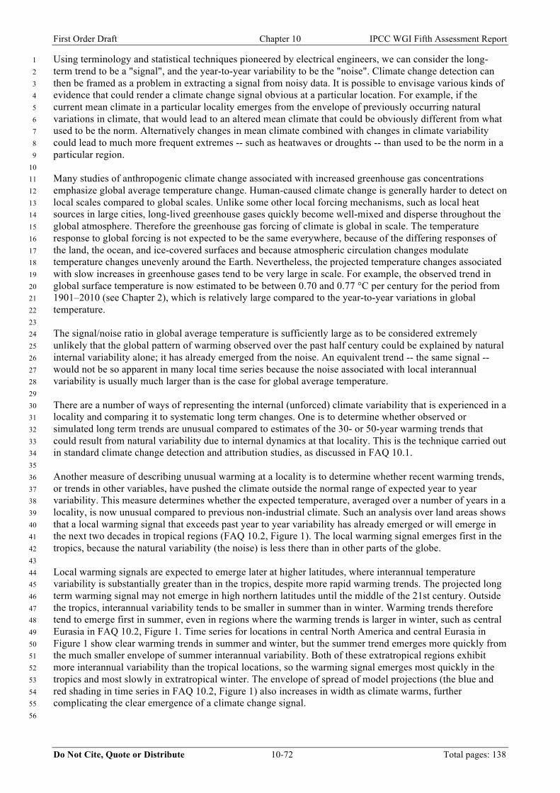
First Order Draft Chapter 10 IPCC WGI Fifth Assessment Report
Do Not Cite, Quote or Distribute 10-72 Total pages: 138
Using terminology and statistical techniques pioneered by electrical engineers, we can consider the long-1 term trend to be a "signal", and the year-to-year variability to be the "noise". Climate change detection can 2 then be framed as a problem in extracting a signal from noisy data. It is possible to envisage various kinds of 3 evidence that could render a climate change signal obvious at a particular location. For example, if the 4 current mean climate in a particular locality emerges from the envelope of previously occurring natural 5 variations in climate, that would lead to an altered mean climate that could be obviously different from what 6 used to be the norm. Alternatively changes in mean climate combined with changes in climate variability 7 could lead to much more frequent extremes -- such as heatwaves or droughts -- than used to be the norm in a 8 particular region. 9 10 Many studies of anthropogenic climate change associated with increased greenhouse gas concentrations 11 emphasize global average temperature change. Human-caused climate change is generally harder to detect on 12 local scales compared to global scales. Unlike some other local forcing mechanisms, such as local heat 13 sources in large cities, long-lived greenhouse gases quickly become well-mixed and disperse throughout the 14 global atmosphere. Therefore the greenhouse gas forcing of climate is global in scale. The temperature 15 response to global forcing is not expected to be the same everywhere, because of the differing responses of 16 the land, the ocean, and ice-covered surfaces and because atmospheric circulation changes modulate 17 temperature changes unevenly around the Earth. Nevertheless, the projected temperature changes associated 18 with slow increases in greenhouse gases tend to be very large in scale. For example, the observed trend in 19 global surface temperature is now estimated to be between 0.70 and 0.77 °C per century for the period from 20 1901–2010 (see Chapter 2), which is relatively large compared to the year-to-year variations in global 21 temperature. 22 23 The signal/noise ratio in global average temperature is sufficiently large as to be considered extremely 24 unlikely that the global pattern of warming observed over the past half century could be explained by natural 25 internal variability alone; it has already emerged from the noise. An equivalent trend -- the same signal -- 26 would not be so apparent in many local time series because the noise associated with local interannual 27 variability is usually much larger than is the case for global average temperature. 28 29 There are a number of ways of representing the internal (unforced) climate variability that is experienced in a 30 locality and comparing it to systematic long term changes. One is to determine whether observed or 31 simulated long term trends are unusual compared to estimates of the 30- or 50-year warming trends that 32 could result from natural variability due to internal dynamics at that locality. This is the technique carried out 33 in standard climate change detection and attribution studies, as discussed in FAQ 10.1. 34 35 Another measure of describing unusual warming at a locality is to determine whether recent warming trends, 36 or trends in other variables, have pushed the climate outside the normal range of expected year to year 37 variability. This measure determines whether the expected temperature, averaged over a number of years in a 38 locality, is now unusual compared to previous non-industrial climate. Such an analysis over land areas shows 39 that a local warming signal that exceeds past year to year variability has already emerged or will emerge in 40 the next two decades in tropical regions (FAQ 10.2, Figure 1). The local warming signal emerges first in the 41 tropics, because the natural variability (the noise) is less there than in other parts of the globe. 42 43 Local warming signals are expected to emerge later at higher latitudes, where interannual temperature 44 variability is substantially greater than in the tropics, despite more rapid warming trends. The projected long 45 term warming signal may not emerge in high northern latitudes until the middle of the 21st century. Outside 46 the tropics, interannual variability tends to be smaller in summer than in winter. Warming trends therefore 47 tend to emerge first in summer, even in regions where the warming trends is larger in winter, such as central 48 Eurasia in FAQ 10.2, Figure 1. Time series for locations in central North America and central Eurasia in 49 Figure 1 show clear warming trends in summer and winter, but the summer trend emerges more quickly from 50 the much smaller envelope of summer interannual variability. Both of these extratropical regions exhibit 51 more interannual variability than the tropical locations, so the warming signal emerges most quickly in the 52 tropics and most slowly in extratropical winter. The envelope of spread of model projections (the blue and 53 red shading in time series in FAQ 10.2, Figure 1) also increases in width as climate warms, further 54 complicating the clear emergence of a climate change signal. 55 56

First Order Draft Chapter 10 IPCC WGI Fifth Assessment Report
Do Not Cite, Quote or Distribute 10-73 Total pages: 138
Assigning a precise date to the future emergence of local anthropogenic warming trends is also subject to 1 uncertainty in future greenhouse gas emissions. A multi-model ensemble forced by a single emissions 2 scenario was used for the results shown in FAQ 10.2, Figure 1. A more or less rapid rate of atmospheric 3 greenhouse gas accumulation would force more or less rapid warming, thereby causing the warming signal 4 to emerge somewhat more or less rapidly from the noise of internal variability. In other words, the spread of 5 model projections depicted by the colored shading in Figure 1 would be considerably greater if different 6 greenhouse gas emissions scenarios were considered. 7 8 Variables other than temperature also show different influences and sensitivities to climate change, such as 9 Arctic sea-ice extent, ocean heat content, ocean salinity and precipitation. Local precipitation trends are very 10 hard to detect, given the large inter-annual variability at most locations, although emergence of trends 11 averaged over a few large continental regions, assessed using techniques similar to that illustrated in FAQ 12 10.2, Figure 1 for temperature, may occur in some regions with pronounced projected trends. For example, 13 projected trends of precipitation increase averaged over Northern Europe, and precipitation decrease 14 averaged over the Mediterranean region, are expected to emerge from internal variability in the 21st Century. 15 16 The preceding paragraphs discuss the detection of projected long-term trends, without explicit regard for the 17 cause of that trend. Attribution of observed changes in climate at local scales to one or more specific causes 18 is complicated by the greater role played by dynamical factors (circulation changes), and determining the 19 effects of external climate forcings other than greenhouse gases. 20 21 Therefore, despite an expectation that climate change has already manifested itself at many localities around 22 the world, attributing the changes at a specific location, and determining with high confidence that a 23 significant fraction of the particularities of the climate evolution in one location can be confidently ascribed 24 to observed greenhouse gas increases, is in many cases still not possible. 25 26 Individual extreme weather events cannot be unambiguously ascribed to climate change since such events 27 could have happened in an unchanged climate. However, the odds of such events could have changed 28 significantly at a particular location, "loading the weather dice", as it were. Statistical modelling may be 29 required to infer from observational data series how the extremes of the distribution are changing, or 30 dynamical modelling to simulate climate states with and without anthropogenic forcings. There is evidence 31 that human-induced increases in greenhouse gases may have contributed substantially to the probability of 32 some heatwaves and may have contributed to the observed intensification of heavy precipitation events 33 found over parts of the northern hemisphere. More clearly, the probability of relatively rare warm summer 34 temperatures (choosing a threshold for summer temperatures as those exceeded one year per decade during 35 the 1961–1990 period) has increased dramatically throughout much of the northern hemisphere and such 36 summers are set to become the norm over the coming decades. The probabilities of other extreme events, 37 including some cold spells, may have been reduced. The probability of many other extreme weather events 38 may not have changed substantially. 39 40 A full answer to the question as to when human influence on climate — as a result of anthropogenic 41 increases in greenhouse gas concentrations — will be obvious on local scales depends on a consideration of 42 what strength of evidence is required to render something obvious to someone. But the most convincing 43 scientific evidence for the effect of climate change on local scales comes from analysing the global picture, 44 and the wealth of evidence from across the climate system linking observed changes to human influence. 45 46 [INSERT FIGURE FAQ 10.2, FIGURE 1 HERE] 47 FAQ 10.2, Figure 1: The map shows the global temperature increase (°C) needed for a single location to undergo a 48 statistically significant change in average summer seasonal surface temperature, aggregated on a country level, based on 49 the SRES A1B scenario. As indicated by the map, tropical countries are associated with the smallest temperature 50 increase (the red colors) required for a statistically significant change. The surrounding time series at four representative 51 locations illustrate geographical and seasonal variations in the emergence of anthropogenically forced temperature 52 change from internal interannual variability of temperature. Above the map, each panel shows extratropical time series 53 of summer season (red) and winter season (blue) temperature at locations in North America and Eurasia from an 54 ensemble of climate model simulations forced by the A1B radiative scenario. The shading about the red and blue curves 55 indicates the 5% and 95% quantiles across all model realizations. Note that the spread of these quantiles widens during 56 the 21st Century as model projections diverge. Interannual variability during an early 20th Century base period (1900–57 1929) (±2 standard deviations) is shaded in gray as an indication of internal variability simulated by the models. 58

First Order Draft Chapter 10 IPCC WGI Fifth Assessment Report
Do Not Cite, Quote or Distribute 10-74 Total pages: 138
Interannual temperature variability is very much larger in winter throughout the extratropics, so the climate change 1 signal emerges more rapidly in summer than in winter, even where the 21st Century temperature trend is greater in 2 winter (as at the Eurasian location in the upper right). Below the map, corresponding time series are shown for locations 3 in tropical South America (left) and tropical Africa (right). In tropical countries, as in the extratropics, the climate 4 change signal emerges from the noise of interannual variability most rapidly in the warm season. Interannual variability 5 is relatively small in the tropics, as shown by how narrow the bands of gray shading are compared to the middle latitude 6 locations above the map, so climate change signals emerge unambiguously from 20th Century variability more quickly 7 in the tropics. Sources: adapted from Mahlstein et al. (2011) and Gutzler and Robbins (2011) 8 9 [END FAQ 10.2 HERE] 10 11 12
13

First Order Draft Chapter 10 IPCC WGI Fifth Assessment Report
Do Not Cite, Quote or Distribute 10-75 Total pages: 138
References 1 2 AchutaRao, K. M., B. D. Santer, P. J. Gleckler, K. E. Taylor, D. W. Pierce, T. P. Barnett, and T. M. L. 3
Wigley, 2006: Variability of ocean heat uptake: Reconciling observations and models. Journal of 4 Geophysical Research, 111, C05019. 5
AchutaRao, K. M., et al., 2007: Simulated and observed variability in ocean temperature and heat content. 6 Proceedings of the National Academy of Sciences, 104, 10768-10773. 7
Adams, J., M. Mann, and C. Ammann, 2003: Proxy evidence for an El Nino-like response to volcanic 8 forcing. Nature, DOI 10.1038/nature02101. 274-278. 9
Ahlmann, H. W., 1948: The present climatic fluctuation. Geographical Journal, 165-195. 10 Alekseev, G., A. Danilov, V. Kattsov, S. Kuz'mina, and N. Ivanov, 2009: Changes in the climate and sea ice 11
of the Northern Hemisphere in the 20th and 21st centuries from data of observations and modeling. 12 Izvestiya Atmospheric and Oceanic Physics, DOI 10.1134/S0001433809060012. 675-686. 13
Alexander, L. V., and J. M. Arblaster, 2009: Assessing trends in observed and modelled climate extremes 14 over Australia in relation to future projections. International Journal of Climatology, 29, 417-435. 15
Allan, R., and T. Ansell, 2006: A new globally complete monthly historical gridded mean sea level pressure 16 dataset (HadSLP2): 1850-2004. Journal of Climate, 19, 5816-5842. 17
Allan, R., and B. Soden, 2007: Large discrepancy between observed and simulated precipitation trends in the 18 ascending and descending branches of the tropical circulation. Geophys. Res. Lett., ARTN L18705, 19 DOI 10.1029/2007GL031460. -. 20
——, 2008: Atmospheric warming and the amplification of precipitation extremes. Science, DOI 21 10.1126/science.1160787. 1481-1484. 22
Allan, R., B. Soden, V. John, W. Ingram, and P. Good, 2010: Current changes in tropical precipitation. 23 Environmental Research Letters, ARTN 025205, DOI 10.1088/1748-9326/5/2/025205. -. 24
Allen, M., 2011: In defense of the traditional null hypothesis: remarks on the Trenberth and Curry WIREs 25 opinion articles. Wiley Interdisciplinary Reviews: Climate Change, 2, 931-934. 26
Allen, M., and S. Tett, 1999: Checking for model consistency in optimal fingerprinting. Climate Dynamics. 27 419-434. 28
Allen, M., and W. Ingram, 2002: Constraints on future changes in climate and the hydrologic cycle. Nature, 29 DOI 10.1038/nature01092. 224-+. 30
Allen, M., and P. Stott, 2003: Estimating signal amplitudes in optimal fingerprinting, part I: theory. Climate 31 Dynamics, DOI 10.1007/s00382-003-0313-9. 477-491. 32
Allen, M., P. Stott, J. Mitchell, R. Schnur, and T. Delworth, 2000: Quantifying the uncertainty in forecasts of 33 anthropogenic climate change. Nature. 617-620. 34
Allen, M., D. Frame, C. Huntingford, C. Jones, J. Lowe, M. Meinshausen, and N. Meinshausen, 2009: 35 Warming caused by cumulative carbon emissions towards the trillionth tonne. Nature, 458, 1163-36 1166. 37
Allen, M. R., 2003: Liability for climate change. 891-892. 38 Ammann, C. M., F. Joos, D. S. Schimel, B. L. Otto-Bliesner, and R. A. Tomas, 2007: Solar influence on 39
climate during the past millennium: Results from transient simulations with the NCAR Climate 40 System Model. Proceedings of the National Academy of Sciences of the United States of America, 104, 41 3713-3718. 42
Anderson, B. T., 2004: Investigation of a large-scale mode of ocean-atmosphere variability and its relation to 43 tropical Pacific sea surface temperature anomalies. Journal of Climate, 17, 4089-4098. 44
Andreae, M., C. Jones, and P. Cox, 2005: Strong present-day aerosol cooling implies a hot future. Nature, 45 DOI 10.1038/nature03671. 1187-1190. 46
Annan, J., and J. Hargreaves, 2006: Using multiple observationally-based constraints to estimate climate 47 sensitivity. Geophys. Res. Lett., ARTN L06704, DOI 10.1029/2005GL025259. -. 48
——, 2010: Reliability of the CMIP3 ensemble. Geophys. Res. Lett., ARTN L02703, DOI 49 10.1029/2009GL041994. -. 50
——, 2011: On the generation and interpretation of probabilistic estimates of climate sensitivity. Clim. 51 Change, 104, 423-436. 52
Aoki, S., N. Bindoff, and J. Church, 2005: Interdecadal water mass changes in the Southern Ocean between 53 30 degrees E and 160 degrees E. Geophys. Res. Lett., ARTN L07607, DOI 10.1029/2004GL022220. -. 54
Armour, K., I. Eisenman, E. Blanchard-Wrigglesworth, K. McCusker, and C. Bitz, 2011: The reversibility of 55 sea ice loss in a state-of-the-art climate model. Geophys. Res. Lett., 38, -. 56

First Order Draft Chapter 10 IPCC WGI Fifth Assessment Report
Do Not Cite, Quote or Distribute 10-76 Total pages: 138
Arzhanov, M. M., A. V. Eliseev, P. F. Demchenko, and I. I. Mokhov, 2007: Modeling of changes in 1 temperature and hydrological regimes of subsurface permafrost, using the climate data (reanalysis). 2 Kriosfera Zemli (Earth Cryosphere), 11, 65-69. 3
Ashok, K., and T. Yamagata, 2009: CLIMATE CHANGE The El Nino with a difference. Nature, 461, 481-4 +. 5
Baker, M., and G. Roe, 2009: The Shape of Things to Come: Why Is Climate Change So Predictable? 6 Journal of Climate, 22, 4574-4589. 7
Barnett, T., D. Pierce, K. Achutarao, P. Gleckler, B. Santer, J. Gregory, and W. Washington, 2005: 8 Penetration of Human-Induced Warming into the World's Oceans. Science, 309, 284-287. 9
Barnett, T. P., et al., 2008: Human-induced changes in the hydrology of the western United States. Science, 10 319, 1080-1083. 11
Beer, J., J. Abreu, and F. Steinhilber, 2009: Sun and planets from a climate point of view. Universal 12 Heliophysical Processes, DOI 10.1017/S1743921309029056. 29-43. 13
Bender, F., 2008: A note on the effect of GCM tuning on climate sensitivity. Environmental Research 14 Letters, ARTN 014001, DOI 10.1088/1748-9326/3/1/014001. -. 15
Bender, F., A. Ekman, and H. Rodhe, 2010: Response to the eruption of Mount Pinatubo in relation to 16 climate sensitivity in the CMIP3 models. Climate Dynamics, DOI 10.1007/s00382-010-0777-3. 875-17 886. 18
Benestad, R. E., and G. A. Schmidt, 2009: Solar trends and global warming. Journal of Geophysical 19 Research-Atmospheres, 114. 20
Bengtsson, L., and K. I. Hodges, 2009: On the evaluation of temperature trends in the tropical troposphere. 21 Clim. Dyn. 22
——, 2011: On the evaluation of temperature trends in the tropical troposphere. Climate Dynamics, 36, 419-23 430. 24
Bengtsson, L., V. Semenov, and O. Johannessen, 2004: The early twentieth-century warming in the Arctic - 25 A possible mechanism. Journal of Climate. 4045-4057. 26
Bengtsson, L., K. I. Hodges, E. Roeckner, and R. Brokopf, 2006: On the natural variability of the pre-27 industrial European climate. Clim Dyn, 27, 17. 28
Bengtsson, L., K. I. Hodges, M. Esch, N. Keenlyside, L. Kornblueh, J. J. Luo, and T. Yamagata, 2007: How 29 may tropical cyclones change in a warmer climate? Tellus.Series A: Dynamic Meteorology and 30 Oceanography, 59(4), 539-561. 31
Berliner, L., R. Levine, and D. Shea, 2000: Bayesian climate change assessment. Journal of Climate. 3805-32 3820. 33
Bhend, J., and H. von Storch, 2008: Consistency of observed winter precipitation trends in northern Europe 34 with regional climate change projections. Climate Dynamics, 31, 17-28. 35
Bindoff, N., and T. McDougall, 2000: Decadal changes along an Indian ocean section at 32 degrees S and 36 their interpretation. Journal of Physical Oceanography. 1207-1222. 37
Bindoff, N. L., et al., 2007: Observations: Oceanic Climate Change and Sea Level. Climate Change 2007: 38 The Physical Science Basis. Contribution of Working Group I to the Fourth Assessment Report of the 39 Intergovernmental Panel on Climate Change, Cambridge University Press. 40
Boe, J., A. Hall, and X. Qu, 2009: September sea-ice cover in the Arctic Ocean projected to vanish by 2100. 41 Nature Geoscience, DOI 10.1038/NGEO467. 341-343. 42
Boer, G., M. Stowasser, and K. Hamilton, 2007: Inferring climate sensitivity from volcanic events. Climate 43 Dynamics, DOI 10.1007/s00382-006-0193-x. 481-502. 44
Boer, G. J., 2011: The ratio of land to ocean temperature change under global warming Climate Dynamics, 45 10.1007/s00382-011-1112-3. 46
Bollasina, M. A., Y. Ming, V. Ramaswamy,, 2011: Anthropogenic Aerosols and the Weakening of the South 47 Asian Summer Monsoon. Science, 10.1126/science.1204994. 48
Bonfils, C., P. B. Duffy, B. D. Santer, T. M. L. Wigley, D. B. Lobell, T. J. Phillips, and C. Doutriaux, 2008: 49 Identification of external influences on temperatures in California. Clim. Change, 87, S43-S55. 50
Booth, B. B. B., P. R. Halloran, and N. J. Dunstone, 2011: Aerosols Implicated as a Prime Driver of 20th 51 century variability within the North Atlantic Nature? 52
Booth, B. B. B., P. R. Halloran, and N. J. Dunstone, 2011: Aerosols Implicated as a Prime Driver of 20th 53 century variability within the North Atlantic. Nature,submitted. 54
Boyer, T., S. Levitus, J. Antonov, R. Locarnini, and H. Garcia, 2005: Linear trends in salinity for the World 55 Ocean, 1955-1998. Geophys. Res. Lett., ARTN L01604, DOI 10.1029/2004GL021791. -. 56

First Order Draft Chapter 10 IPCC WGI Fifth Assessment Report
Do Not Cite, Quote or Distribute 10-77 Total pages: 138
Brayshaw, D. J., B. Hoskins, and M. Blackburn, 2008: he Storm-Track Response to Idealized SST 1 Perturbations in an Aquaplanet GCM. Journal of Atmospheric Sciences, 65, 2842–2860. 2
Brohan, P., J. J. Kennedy, I. Harris, S. F. B. Tett, and P. D. Jones, 2006: Uncertainty estimates in regional 3 and global observed temperature changes: A new data set from 1850. Journal of Geophysical 4 Research-Atmospheres, 111. 5
Bronnimann, S., 2009: Early twentieth-century warming. Nature Geoscience, DOI 10.1038/ngeo670. 735-6 736. 7
Brown, R., and P. Mote, 2009: The Response of Northern Hemisphere Snow Cover to a Changing Climate. 8 Journal of Climate, DOI 10.1175/2008JCLI2665.1. 2124-2145. 9
Brown, S. J., J. Caesar, and C. A. T. Ferro, 2008: Global changes in extreme daily temperature since 1950. 10 Journal of Geophysical Research-Atmospheres, 113. 11
Burke, E. J., S. J. Brown, and N. Christidis, 2006: Modeling the recent evolution of global drought and 12 projections for the twenty-first century with the Hadley Centre climate model. Journal of 13 Hydrometeorology, 7(5), 1113-1125. 14
Butchart, N., et al., 2011: Multimodel climate and variability of the stratosphere. Journal of Geophysical 15 Research-Atmospheres, 116. 16
Butler, A. H., D. W. Thompson, and R. Heikes, 2010: The steady-state atmospheric circulation resions to 17 1021 climate change-like thermal forcings in a simple general circulation model. Journal of Climate, 18 23, 23. 19
Cai, W., T. Cowan, and A. Sullivan, 2009: Recent unprecedented skewness towards positive Indian Ocean 20 Dipole occurrences and its impact on Australian rainfall. Geophys. Res. Lett., 36. 21
Camp, C., and K. Tung, 2007: Surface warming by the solar cycle as revealed by the composite mean 22 difference projection. Geophys. Res. Lett., 34, -. 23
Cayan, D. R., T. Das, D. W. Pierce, T. P. Barnett, M. Tyree, and A. Gershunov, 2010: Future dryness in the 24 southwest US and the hydrology of the early 21st century drought. Proceedings of the National 25 Academy of Sciences, 107, 21271-21276. 26
Cazenave, A., and W. Llovel, 2010: Contemporary Sea Level Rise. Annual Review of Marine Science, 2, 27 145-173. 28
Chang, P., et al., 2007: Pacific meridional mode and El Nino-southern oscillation. Geophys. Res. Lett., 34. 29 Chen, G., Y. Ming, N. D. Singer, and J. Lu, 2011: Testing the Clausius-Clapeyron constraint on the 30
aerosol-induced changes in mean and extreme precipitation. Geophys. Res. Lett., 38. 31 Cheng, G., and T. Wu, 2007: Responses of permafrost to climate change and their environmental 32
significance, Qinghai-Tibet Plateau. Journal of Geophysical Research, 112. 33 Chinn, T., S. Winkler, M. Salinger, and N. Haakensen, 2005: Srecent glacier advances in Norway and New 34
Zealand: A comparison of their glaciological and meteorological causes. Geografiska Annaler Series 35 a-Physical Geography. 141-157. 36
Choi, G., D. Robinson, and S. Kang, 2010: Changing Northern Hemisphere Snow Seasons. Journal of 37 Climate, DOI 10.1175/2010JCLI3644.1. 5305-5310. 38
Christidis, N., P. A. Stott, and S. J. Brown, 2011a: The role of human activity in the recent warming of 39 extremely warm daytime temperatures. 40
Christidis, N., P. A. Stott, F. W. Zwiers, H. Shiogama, and T. Nozawa, 2010: Probabilistic estimates of 41 recent changes in temperature: a multi-scale attribution analysis. Climate Dynamics, 34, 1139-1156. 42
Christidis, N., P. A. Stott, G. S. Jones, H. Shiogama, T. Nozawa, and J. Luterbacher, 2011b: Human activity 43 and anomalously warm seasons in Europe. International Journal of Climatology, 10.1002/joc.2262. 44
Christy, J. R., et al., 2010: What do observational datasets say about modeled tropospheric temperature 45 trends since 1979? Remote Sens., 2, 2148-2169. 46
Chung, E., B. Soden, and B. Sohn, 2010: Revisiting the determination of climate sensitivity from 47 relationships between surface temperature and radiative fluxes. Geophys. Res. Lett., ARTN L10703, 48 DOI 10.1029/2010GL043051. -. 49
Church, J., N. White, and J. Arblaster, 2005: Significant decadal-scale impact of volcanic eruptions on sea 50 level and ocean heat content. Nature, 438, 74-77. 51
Church, J., et al., 2011: Revisiting the Earth's sea-level and energy budgets from 1961 to 2008. Geophys. 52 Res. Lett., 38, -. 53
Chylek, P., and U. Lohmann, 2008a: Aerosol radiative forcing and climate sensitivity deduced from the last 54 glacial maximum to Holocene transition. Geophys. Res. Lett., ARTN L04804, DOI 55 10.1029/2007GL032759. -. 56

First Order Draft Chapter 10 IPCC WGI Fifth Assessment Report
Do Not Cite, Quote or Distribute 10-78 Total pages: 138
——, 2008b: Reply to comment by Andrey Ganopolski and Thomas Schneider von Deimling on "Aerosol 1 radiative forcing and climate sensitivity deduced from the Last Glacial Maximum to Holocene 2 transition''. Geophys. Res. Lett., ARTN L23704, DOI 10.1029/2008GL034308. -. 3
Chylek, P., U. Lohmann, M. Dubey, M. Mishchenko, R. Kahn, and A. Ohmura, 2007: Limits on climate 4 sensitivity derived from recent satellite and surface observations. Journal of Geophysical Research-5 Atmospheres, 112. 6
Comiso, J., and F. Nishio, 2008: Trends in the sea ice cover using enhanced and compatible AMSR-E, 7 SSM/I, and SMMR data. Journal of Geophysical Research-Oceans, ARTN C02S07, DOI 8 10.1029/2007JC004257. -. 9
Cook, E., R. Seager, M. Cane, and D. Stahle, 2007: North American drought: Reconstructions, causes, and 10 consequences. Earth-Science Reviews, DOI 10.1016/j.earscirev.2006.12.002. 93-134. 11
Cordero, E. C., and P. M. D. Forster, 2006: Stratospheric variability and trends in models used for the IPCC 12 AR4. Atmospheric Chemistry and Physics, 6, 5369-5380. 13
Cravatte, S., T. Delcroix, D. Zhang, M. McPhaden, and J. Leloup, 2009: Observed freshening and warming 14 of the western Pacific Warm Pool. Climate Dynamics, DOI 10.1007/s00382-009-0526-7. 565-589. 15
Crook, J., P. Forster, and N. Stuber, 2011: Spatial Patterns of Modeled Climate Feedback and Contributions 16 to Temperature Response and Polar Amplification. Journal of Climate, 24, 3575-3592. 17
Curry, J., 2011: Nullifying the climate null hypothesis. Wiley Interdisciplinary Reviews: Climate Change, 2, 18 919-924. 19
Curry, J. A., and P. J. Webster, 2011: Climate Science and the Uncertainty Monster. Bulletin of the American 20 Meteorological Society, 10.1175/2011BAMS3139.1. in press. 21
Curry, R., B. Dickson, and I. Yashayaev, 2003: A change in the freshwater balance of the Atlantic Ocean 22 over the past four decades. Nature, DOI 10.1038/nature02206. 826-829. 23
Dai, A., 2011: Drought under global warming: a review. Wiley Interdisciplinary Reviews: Climate Change, 24 2, 21. 25
Dai, A., T. Qian, K. Trenberth, and J. Milliman, 2009: Changes in continental freshwater discharge from 26 1948 to 2004. Journal of Climate, 22, 2773-2792. 27
Dall'Amico, M., L. J. Gray, K. H. Rosenlof, A. A. Scaife, K. P. Shine, and P. A. Stott, 2010: Stratospheric 28 temperature trends: impact of ozone variability and the QBO. Climate Dynamics, 34, 381-398. 29
Davis, S. M., and K. H. Rosenlof, 2011: A multi-diagnostic intercomparision of tropical width and jet 30 timeseries using meteorological reanalyses and satellite observations. J.Climate, in press. 31
Dean, S. M., and P. A. Stott, 2009: The Effect of Local Circulation Variability on the Detection and 32 Attribution of New Zealand Temperature Trends. Journal of Climate, 22, 6217-6229. 33
DelSole, T., M. K. Tippett, and J. Shukla, 2011: A significant component of unforced multidecadal 34 variability in the recent acceleration of global warming. Journal of Climate, 24, 18. 35
Delworth, T., and M. Mann, 2000: Observed and simulated multidecadal variability in the Northern 36 Hemisphere. Climate Dynamics, 16, 661-676. 37
Delworth, T., V. Ramaswamy, and G. Stenchikov, 2005: The impact of aerosols on simulated ocean 38 temperature and heat content in the 20th century. Geophys. Res. Lett., 32, L24709. 39
Delworth, T. L., and T. R. Knutson, 2000: Simulation of Early 20th Century Global Warming. Science, 287, 40 5. 41
Deo, R. C., J. I. Syktus, C. A. McAlpine, P. J. Lawrence, H. A. McGowan, and S. R. Phinn, 2009: Impact of 42 historical land cover change on daily indices of climate extremes including droughts in eastern 43 <country-region>Australia</country-region>. Geophys. Res. Lett., 36(L08705). 44
Dery, S. J., and R. D. Brown, 2007: Recent Northern Hemisphere snow cover extenet trends and implications 45 for the snow-albedo feedback. Geophys. Res. Lett., 34, 6. 46
Deser, C., and H. Teng, 2008: Evolution of Arctic sea ice concentration trends and the role of atmospheric 47 circulation forcing, 1979-2007. Geophys. Res. Lett., ARTN L02504, DOI 10.1029/2007GL032023. 48
Deser, C., A. S. Phillips, and M. A. Alexander, 2010: Twentieth century tropical sea surface temperature 49 trends revisited. Geophys. Res. Lett., 37. 50
Deutsch, C., S. Emerson, and L. Thompson, 2005: Fingerprints of climate change in North Pacific oxygen 51 (vol 32, art no L16604, 2005). Geophys. Res. Lett., ARTN L17610, DOI 10.1029/2005GL024471. -. 52
Dickson, R., et al., 2000: The Arctic Ocean response to the North Atlantic oscillation. Journal of Climate. 53 2671-2696. 54
Ding, Q., E. Steig, D. Battisti, and M. Kuttel, 2011: Winter warming in West Antarctica caused by central 55 tropical Pacific warming. Nature Geoscience, 4, 398-403. 56

First Order Draft Chapter 10 IPCC WGI Fifth Assessment Report
Do Not Cite, Quote or Distribute 10-79 Total pages: 138
Doherty, S., et al., 2009: LESSONS LEARNED FROM IPCC AR4 Scientific Developments Needed To 1 Understand, Predict, And Respond To Climate Change. Bulletin of the American Meteorological 2 Society, DOI 10.1175/2008BAMS2643.1. 497-+. 3
Dole, R., et al., 2011: Was there a basis for anticipating the 2010 Russian heat wave? Geophys. Res. Lett., 38. 4 Domingues, C., J. Church, N. White, P. Gleckler, S. Wijffels, P. Barker, and J. Dunn, 2008: Improved 5
estimates of upper-ocean warming and multi-decadal sea-level rise. Nature, 453, 1090-1093. 6 Doscher, R., K. Wyser, H. Meier, M. Qian, and R. Redler, 2010: Quantifying Arctic contributions to climate 7
predictability in a regional coupled ocean-ice-atmosphere model. Climate Dynamics, DOI 8 10.1007/s00382-009-0567-y. 1157-1176. 9
Douglass, D., E. Blackman, and R. Knox, 2004: Temperature response of Earth to the annual solar irradiance 10 cycle (vol 323, pg 315, 2004). Physics Letters a, DOI 10.1016/j.physleta.2004.03.029. 175-176. 11
Douglass, D. H., J. R. Christy, B. D. Pearson, and S. F. Singer, 2008: A comparison of tropical temperature 12 trends with model predictions. International Journal of Climatology, 28, 1693-1701. 13
Drost, F., D. Karoly, and K. Braganza, 2011: Communicating global climate change using simple indices: an 14 update Climate Dynamics, 10.1007/s00382-011-1227-6. 15
Durack, P., and S. Wijffels, 2010: Fifty-Year Trends in Global Ocean Salinities and Their Relationship to 16 Broad-Scale Warming. Journal of Climate, DOI 10.1175/2010JCLI3377.1. 4342-4362. 17
Durack, P. J., S. E. Wijffels, and R. J. Matear, 2011a (submitted): Ocean Salinities Reveal Strong Global 18 Water Cycle Intensification during 1950-2000., Science. 19
——, 2011b (submitted): Ocean Salinities Reveal Strong Global Water Cycle Intensification during 1950-20 2000., Science. 21
Dutton, J. F., C. J. Poulsen, and J. L. Evans, 2000: The effect of global climate change on the regions of 22 tropical convection in CSM1. Geophys. Res. Lett., 27(19), 3049-3052. 23
Easterling, D. R., and M. F. Wehner, 2009: Is the climate warming or cooling? Geophys. Res. Lett., 36. 24 Edwards, T., M. Crucifix, and S. Harrison, 2007: Using the past to constrain the future: how the palaeorecord 25
can improve estimates of global warming. Progress in Physical Geography, DOI 26 10.1177/0309133307083295. 481-500. 27
Eliseev, A. V., M. M. Arzhanov, P. E. Demchenko, and I. I. Mokhov, 2009: 2009: Changes in climatic 28 characteristics of Northern Hemisphere extratropical land in the 21st century: Assessments with the 29 IAP RAS climate model. Izvestiya, Atmos. Ocean. Phys., 45, 271-283. 30
Elsner, J. B., 2006: Evidence in support of the climate change–Atlantic hurricane hypothesis. Geophys. Res. 31 Lett. 32
Elsner, J. B., J. P. Kossin, and T. H. Jagger, 2008: The increasing intensity of the strongest tropical cyclones. 33 Nature, 455(7209). 34
Emanuel, K., 2000: A statistical analysis of tropical cyclone intensity. Monthly Weather Review, 128(4), 35 1139-1152. 36
——, 2005: Increasing destructiveness of tropical cyclones over the past 30 years. Nature, 436, 686-688. 37 Emerson, S., Y. Watanabe, T. Ono, and S. Mecking, 2004: Temporal trends in apparent oxygen utilization in 38
the upper pycnocline of the North Pacific: 1980-2000. Journal of Oceanography. 139-147. 39 Emori, S., and S. J. Brown, 2005: Dynamic and thermodynamic changes in mean and extreme precipitation 40
under changed climate. Geophys. Res. Lett., 32(L17706). 41 Eyring, V., T. G. Shepherd, and D. W. Waugh, 2010: SPARC Report on the Evaluation of Chemistry-42
Climate Models,. WCRP-132, WMO/TD-No. 1526. 43 Eyring, V., et al., 2006: Assessment of temperature, trace species, and ozone in chemistry-climate model 44
simulations of the recent past. Journal of Geophysical Research-Atmospheres, 111. 45 Feldstein, S., 2002: The recent trend and variance increase of the annular mode. Journal of Climate. 88-94. 46 Feng, S., R. J. Oglesby, C. M. Rowe, D. B. Loope, and Q. Hu, 2008: Atlantic and Pacific SST influences on 47
Medieval drought in North America simulated by the Community Atmospheric Model. Journal of 48 Geophysical Research-Atmospheres, 113. 49
Fettweis, X., G. Mabille, M. Erpicum, S. Nicolay, and M. Van den Broeke, 2011: The 1958-2009 Greenland 50 ice sheet surface melt and the mid-tropospheric atmospheric circulation. Climate Dynamics, DOI 51 10.1007/s00382-010-0772-8. 139-159. 52
Feudale, L., and J. Shukla, 2007: Role of Mediterranean SST in enhancing the European heat wave of 53 summer 2003. Geophys. Res. Lett., 34. 54
——, 2010: Influence of sea surface temperature on the European heat wave of 2003 summer. Part I: an 55 observational study. Clim. Dyn., DOI 10.1007/s00382-010-0788-0. 56

First Order Draft Chapter 10 IPCC WGI Fifth Assessment Report
Do Not Cite, Quote or Distribute 10-80 Total pages: 138
Fischer, E. M., and C. Schär 2010: Consistent geographical patterns of changes in high-impact European 1 heatwaves. Nature Geoscience, 3, 398-403. 2
Fischer, E. M., S. I. Seneviratne, P. L. Vidale, D. Luthi, and C. Schar, 2007: Soil moisture - Atmosphere 3 interactions during the 2003 European summer heat wave. Journal of Climate, 20, 5081-5099. 4
Fogt, R., J. Perlwitz, A. Monaghan, D. Bromwich, J. Jones, and G. Marshall, 2009: Historical SAM 5 Variability. Part II: Twentieth-Century Variability and Trends from Reconstructions, Observations, 6 and the IPCC AR4 Models. Journal of Climate, DOI 10.1175/2009JCLI2786.1. 5346-5365. 7
Folland, C. K., et al., 2011: High predictive skill of global surface temperature a year ahead. Met Office 8 Hadley Centre Climate Programme (MOHCCP) 2010-2012, Met Office Hadley Centre, 21. 9
Forest, C., P. Stone, and A. Sokolov, 2006: Estimated PDFs of climate system properties including natural 10 and anthropogenic forcings. Geophys. Res. Lett., ARTN L01705, DOI 10.1029/2005GL023977. -. 11
——, 2008: Constraining climate model parameters from observed 20th century changes. Tellus Series a-12 Dynamic Meteorology and Oceanography, DOI 10.1111/j.1600-0870.2008.00346.x. 911-920. 13
Forest, C., P. Stone, A. Sokolov, M. Allen, and M. Webster, 2002: Quantifying uncertainties in climate 14 system properties with the use of recent climate observations. Science. 113-117. 15
Forster, P., and K. Taylor, 2006: Climate forcings and climate sensitivities diagnosed from coupled climate 16 model integrations. Journal of Climate, 19, 6181-6194. 17
Forster, P., and J. Gregory, 2006: The climate sensitivity and its components diagnosed from Earth Radiation 18 Budget data. Journal of Climate. 39-52. 19
Forster, P. M., et al., 2011: Stratospheric changes and climate, Chapter 4 in Scientific Assessment of Ozone 20 Depletion: 2010. Global Ozone Research and Monitoring Project-Report No. 52, P. M. Forster, et al., 21 Ed., World Meteorological Organization, 516pp. 22
Foukal, P., C. Frohlich, H. Spruit, and T. Wigley, 2006: Variations in solar luminosity and their effect on the 23 Earth's climate. Nature, 443, 161-166. 24
Fowler, H. J., and R. L. Wilby, 2010: Detecting changes in seasonal precipitation extremes using regional 25 climate model projections: Implications for managing fluvial flood risk. Water Resources Research, 26 46(W0525). 27
Frame, D., D. Stone, P. Stott, and M. Allen, 2006: Alternatives to stabilization scenarios. Geophys. Res. 28 Lett., ARTN L14707, DOI 10.1029/2006GL025801. -. 29
Frame, D., B. Booth, J. Kettleborough, D. Stainforth, J. Gregory, M. Collins, and M. Allen, 2005: 30 Constraining climate forecasts: The role of prior assumptions. Geophys. Res. Lett., ARTN L09702, 31 DOI 10.1029/2004GL022241. -. 32
Frank, D. C., J. Esper, C. C. Raible, U. Buntgen, V. Trouet, B. Stocker, and F. Joos, 2010: Ensemble 33 reconstruction constraints on the global carbon cycle sensitivity to climate, 463, 6. 34
Franzke, C., 2010: Long-Range Dependence and Climate Noise Characteristics of Antarctic Temperature 35 Data. Journal of Climate, DOI 10.1175/2010JCLI3654.1. 6074-6081. 36
Free, M., 2011: The Seasonal Structure of Temperature Trends in the Tropical Lower Stratosphere. Journal 37 of Climate, 24, 859-866. 38
Frierson, D., J. Lu, and G. Chen, 2007: Width of the Hadley cell in simple and comprehensive general 39 circulation models. Geophys. Res. Lett., ARTN L18804, DOI 10.1029/2007GL031115. -. 40
Frierson, D. M. W., 2006: Robust increases in midlatitude static stability in simulations of global warming. 41 Geophys. Res. Lett., 33. 42
Fu, Q., and P. Lin, 2011: Poleward shift of subtropical jets inferred from satellite-observed lower 43 stratospheric temperatures. J. Climate, 24, 5597-5603. 44
Fu, Q., S. Solomon, and P. Lin, 2010: On the seasonal dependence of tropical lower-stratospheric 45 temperature trends. Atmospheric Chemistry and Physics, 10, 2643-2653. 46
Fu, Q., S. Manabe, and C. M. Johanson, 2011: On the warming in the tropical upper troposphere: Models 47 versus observations. Geophys. Res. Lett., 38. 48
Fu, Q., C. M. Johanson, J. M. Wallace, and T. Reichler, 2006: Enhanced mid-latitude tropospheric warming 49 in satellite measurements. Science, 312, 1179-1179. 50
Fyfe, J., 2006: Southern Ocean warming due to human influence. Geophys. Res. Lett., 33, -. 51 Fyfe, J. C., N. P. Gillett, and D. W. J. Thompson, 2010: Comparing variability and trends in observed and 52
modelled global-mean surface temperature. Geophys. Res. Lett., 37. 53 Fyfe, J. C., M. J. Merryfield, V. Kharin, G. J. Boer, W.-S. Lee, and K. v. Salzen, 2011: Skillful predictions of 54
decadal trends in global mean surface temperatur. Geophys. Res. Lett., 38. 55 Gadgil, S., and K. R. Kumar, 2006: The Asian Monsoon. Springer/Praxis Publishing, 651-682 pp. 56

First Order Draft Chapter 10 IPCC WGI Fifth Assessment Report
Do Not Cite, Quote or Distribute 10-81 Total pages: 138
Ganopolski, A., and T. Schneider von Deimling, 2008: Comment on "Aerosol radiative forcing and climate 1 sensitivity deduced from the Last Glacial Maximum to Holocene transition'' by Petr Chylek and Ulrike 2 Lohmann. Geophys. Res. Lett., ARTN L23703, DOI 10.1029/2008GL033888. -. 3
Gascard, J. C., and e. al, 2008: Exploring Arcitc transpolar drift during dramatic sea ice retreat. EOS, 89, 3. 4 Gedney, N., P. M. Cox, R. A. Betts, O. Boucher, C. Huntingford, and P. A. Stott, 2006: Detection of a direct 5
carbon dioxide effect in continental river runoff records. Nature, 439, 835-838. 6 Giannini, A., R. Saravanan, and P. Chang, 2003: Oceanic forcing of Sahel rainfall on interannual to 7
interdecadal time scales. Science, 302, 1027-1030. 8 Giese, B. S., and S. Ray, 2011: El Nino variability in simple ocean data assimilation (SODA), 1871-2008. 9
Journal of Geophysical Research-Oceans, 116. 10 Giles, K., S. Laxon, and A. Ridout, 2008: Circumpolar thinning of Arctic sea ice following the 2007 record 11
ice extent minimum. Geophys. Res. Lett., ARTN L22502, DOI 10.1029/2008GL035710. -. 12 Gillett, N., 2005: Climate modelling - Northern Hemisphere circulation. Nature, DOI 10.1038/437496a. 496-13
496. 14 Gillett, N., and P. Stott, 2009: Attribution of anthropogenic influence on seasonal sea level pressure. 15
Geophys. Res. Lett., ARTN L23709, DOI 10.1029/2009GL041269. -. 16 Gillett, N., A. Weaver, F. Zwiers, and M. Wehner, 2004: Detection of volcanic influence on global 17
precipitation. Geophys. Res. Lett., ARTN L12217, DOI 10.1029/2004GL020044. -. 18 Gillett, N. P., R. J. Allan, and T. J. Ansell, 2005: Detection of external influence on sea level pressure with a 19
multi-model ensemble. Geophys. Res. Lett., 32(L19714). 20 Gillett, N. P., P. A. Stott, and B. D. Santer, 2008a: Attribution of cyclogenesis region sea surface temperature 21
change to anthropogenic influence. Geophys. Res. Lett., 35. 22 Gillett, N. P., G. C. Hegerl, M. R. Allen, and P. A. Stott, 2000: Implications of changes in the Northern 23
Hemisphere circulation for the detection of anthropogenic climate change. Geophys. Res. Lett., 27, 24 993-996. 25
Gillett, N. P., V. K. Arora, G. M. Flato, J. F. Scinocca, and K. von Salzen, 2011a: Improved constraints on 26 21st-century warming derived using 160 years of temperature observations. Geophys. Res. Lett. 27
Gillett, N. P., et al., 2008b: Attribution of polar warming to human influence. Nature Geoscience, 1, 750-28 754. 29
Gillett, N. P., et al., 2011b: Attribution of observed changes in stratospheric ozone and temperature. Atmos. 30 Chem. Phys, 599-609. 31
Gleckler, P. J., T. M. L. Wigley, B. D. Santer, J. M. Gregory, K. AchutaRao, and K. E. Taylor, 2006: 32 Volcanoes and climate: Krakatoa's signature persists in the ocean. Nature, 439, 675-675. 33
Gleckler, P. J., et al., 2011: Human-induced ocean warming identified with improved observations in a 34 multi-model analysis. Nature, submitted. 35
Gong, D. Y., and C. H. Ho, 2002: The Siberian High and climate change over middle to high latitude Asia. 36 Theoretical and Applied Climatology, 72, 1-9. 37
Goosse, H., W. Lefebvre, A. de Montety, E. Crespin, and A. Orsi, 2009: Consistent past half-century trends 38 in the atmosphere, the sea ice and the ocean at high southern latitudes. Climate Dynamics, DOI 39 10.1007/s00382-008-0500-9. 999-1016. 40
Goosse, H., J. Guiot, M. E. Mann, S. Dubinkina, and Y. Sallaz-Damaz, 2011a: The medieval climate 41 anomaly in Europe: Comparison of the summer and annual mean signals in two reconstructions and in 42 simulations with data assimilation. Global and Planetary Change. 43
Goosse, H., E. Crespin, A. de Montety, M. Mann, H. Renssen, and A. Timmermann, 2010: Reconstructing 44 surface temperature changes over the past 600 years using climate model simulations with data 45 assimilation. Journal of Geophysical Research-Atmospheres, ARTN D09108, DOI 46 10.1029/2009JD012737. -. 47
Goosse, H., et al., 2011b: The Role of Forcing and Internal Dynamics in 5 Explaining the “Medieval Climate 48 Anomaly”. Climate Dynamics. 49
Goosse, H., et al., 2006: The origin of the European "Medieval Warm Period". Clim. Past., 99-113. 50 Gouretski, V., and K. Koltermann, 2007: How much is the ocean really warming? Geophys. Res. Lett., 34, 51
L01610. 52 Grant, A., S. Bronnimann, T. Ewen, T. Griesser, and A. Stickler, 2009: The early twentieth century warm 53
period in the European Arctic. Meteorologische Zeitschrift, 18, 425-432. 54 Graversen, R., and M. Wang, 2009: Polar amplification in a coupled climate model with locked albedo. 55
Climate Dynamics, DOI 10.1007/s00382-009-0535-6. 629-643. 56 Gray, L., et al., 2010: SOLAR INFLUENCES ON CLIMATE. Reviews of Geophysics, 48, -. 57

First Order Draft Chapter 10 IPCC WGI Fifth Assessment Report
Do Not Cite, Quote or Distribute 10-82 Total pages: 138
Gregory, J., 2000: Vertical heat transports in the ocean and their effect an time-dependent climate change. 1 Climate Dynamics. 501-515. 2
Gregory, J., J. Lowe, and S. Tett, 2006: Simulated global-mean sea level changes over the last half-3 millennium. Journal of Climate, 19, 4576-4591. 4
Gregory, J. M., H. T. Banks, P. A. Stott, J. A. Lowe, and M. D. Palmer, 2004: Simulated and observed 5 decadal variability in ocean heat content. Geophys. Res. Lett., 31, L15312. 6
Guilyardi, E., 2006: El Nino-mean state-seasonal cycle interactions in a multi-model ensemble. Climate 7 Dynamics, 26, 329-348. 8
Gutowski, W. J., et al., 2008: Causes of Observed Changes in Extremes and Projections of Future Changes. 9 Weather and Climate Extremes in a Changing Climate. Regions of Focus: North America, Hawaii, 10 Caribbean, and U.S. Pacific Islands, T. R. Karl, et al., Ed., A Report by the U.S. Climate Change 11 Science Program and the Subcommittee on Global Change Research. 12
Gutzler, D. S., and T. O. Robbins, 2011: Climate variability and projected change in the western United 13 States: regional downscaling and drought statistics. Climate Dynamics, 37, 835-849. 14
Haerter, J. O., and P. Berg, 2009: Unexpected rise in extreme precipitation caused by a shift in rain type? 15 Nature Geoscience, 2(6), 372-373. 16
Haimberger, L., C. Tavolato, and S. Sperka, 2011: On the persistence of a tropical tropospheric warming 17 maximum during five decades of radiosonde observations. submitted to Science. 18
Han, W., et al., 2010: Patterns of Indian Ocean sea-level change in a warming climate. Nature Geoscience, 3, 19 546-550. 20
Hanna, E., et al., 2008: Increased runoff from melt from the Greenland Ice Sheet: A response to global 21 warming. Journal of Climate, 21, 331-341. 22
Hannart, A., J. Dufresne, and P. Naveau, 2009: Why climate sensitivity may not be so unpredictable. 23 Geophys. Res. Lett., ARTN L16707, DOI 10.1029/2009GL039640. -. 24
Hansen, and e. al, 2011 (Submitted): Earth's Energy Imbalance and Implications. Atmos. Chem Phys 25 Discuss, 27031-27105. 26
HANSEN, J., and S. LEBEDEFF, 1987: GLOBAL TRENDS OF MEASURED SURFACE AIR-27 TEMPERATURE. Journal of Geophysical Research-Atmospheres. 13345-13372. 28
Hansen, J., R. Ruedy, M. Sato, and K. Lo, 2010: GLOBAL SURFACE TEMPERATURE CHANGE. 29 Reviews of Geophysics, 48. 30
Hansen, J., et al., 2001: A closer look at United States and global surface temperature change. Journal of 31 Geophysical Research-Atmospheres, 106, 23947-23963. 32
Hansen, J., et al., 2005a: Earth's energy imbalance: Confirmation and implications. Science, DOI 33 10.1126/science.1110252. 1431-1435. 34
Hansen, J., et al., 2005b: Efficacy of climate forcings. Journal of Geophysical Research-Atmospheres, 110. 35 Hargreaves, J., A. Abe-Ouchi, and J. Annan, 2007: Linking glacial and future climates through an ensemble 36
of GCM simulations. Clim. Past., 77-87. 37 Harries, J., and C. Belotti, 2010: On the Variability of the Global Net Radiative Energy Balance of the 38
Nonequilibrium Earth. Journal of Climate, DOI 10.1175/2009JCLI2797.1. 1277-1290. 39 HASSELMANN, K., 1976: STOCHASTIC CLIMATE MODELS .1. THEORY. Tellus, 28, 473-485. 40 ——, 1997: Multi-pattern fingerprint method for detection and attribution of climate change. Climate 41
Dynamics. 601-611. 42 Hegerl, G., and F. Zwiers, 2011: Use of models in detection and attribution of climate change. Wiley. 43 Hegerl, G., T. Crowley, W. Hyde, and D. Frame, 2006a: Climate sensitivity constrained by temperature 44
reconstructions over the past seven centuries. Nature, DOI 10.1038/nature04679. 1029-1032. 45 Hegerl, G., T. Crowley, S. Baum, K. Kim, and W. Hyde, 2003: Detection of volcanic, solar and greenhouse 46
gas signals in paleo-reconstructions of Northern Hemispheric temperature. Geophys. Res. Lett., ARTN 47 1242, DOI 10.1029/2002GL016635. -. 48
Hegerl, G., J. Luterbacher, F. Gonzalez-Rouco, S. F. B. Tett, T. Crowley, and E. Xoplaki, 2011a: Influence 49 of human and natural forcing on European seasonal temperatures. Nature Geoscience, published 50 online 16 January 2011, 5. 51
Hegerl, G., T. Crowley, M. Allen, W. Hyde, H. Pollack, J. Smerdon, and E. Zorita, 2007a: Detection of 52 human influence on a new, validated 1500-year temperature reconstruction. Journal of Climate, DOI 53 10.1175/JCLI4011.1. 650-666. 54
Hegerl, G., et al., 2006b: Climate change detection and attribution: Beyond mean temperature signals. 55 Journal of Climate. 5058-5077. 56

First Order Draft Chapter 10 IPCC WGI Fifth Assessment Report
Do Not Cite, Quote or Distribute 10-83 Total pages: 138
Hegerl, G. C., F. W. Zwiers, and C. Tebaldi, 2011b: Patterns of change: Whose fingerprint is seen in global 1 warming? Environmental Research Letters. 2
Hegerl, G. C., P. Stott, S. Solomon, and F. W. Zwiers, 2011c: Comment on Climate Science and the 3 Uncertainty Monster by J.A. Curry and P.J. Webster. Bulletin of the American Meteorological Society, 4 in press. 5
Hegerl, G. C., et al., 2010: Good Practice Guidance Paper on Detection and Attribution Related to 6 Anthropogenic Climate Change. 7
Hegerl, G. C., et al., 2007b: Understanding and Attributing Climate Change. Climate Change 2007: The 8 Physical Science Basis. Contribution of Working Group I to the Fourth Assessment Report of the 9 Intergovernmental Panel on Climate Change, Cambridge University Press. 10
Hegerl, G. C., et al., 2007b: Understanding and Attributing climate change, climate change 2007: The 11 Physical Science Basis. Contribution of Working Group I to the Fourth Assessment Report of the 12 Intergovernment Panel on Climate Change., Cambridge University Press, Cambridge, United 13 Kingdom and New York, USA. 14
Held, I., and B. Soden, 2006a: Robust responses of the hydrological cycle to global warming. Journal of 15 Climate. 5686-5699. 16
Held, I., M. Winton, K. Takahashi, T. Delworth, F. Zeng, and G. Vallis, 2010: Probing the Fast and Slow 17 Components of Global Warming by Returning Abruptly to Preindustrial Forcing. Journal of Climate, 18 DOI 10.1175/2009JCLI3466.1. 2418-2427. 19
Held, I. M., 2000: The general circulation of the atmosphere, 70 pp. 20 Held, I. M., and B. J. Soden, 2006b: Robust responses of the hydrological cycle to global warming. Journal 21
of Climate, 19, 5686-5699. 22 Helm, K., N. Bindoff, and J. Church, 2010a: Changes in the global hydrological-cycle inferred from ocean 23
salinity. Geophys. Res. Lett., ARTN L18701, DOI 10.1029/2010GL044222. -. 24 ——, 2010b: Changes in the global hydrological-cycle inferred from ocean salinity. Geophysical Research 25
Letters, 37, -. 26 Helm, K. P., N. L. Bindoff, and J. A. Church, 2011: Observed decreases in oxygen content of the global 27
ocean. Geophysical research letters. 28 Henriksson, S., E. Arjas, M. Laine, J. Tamminen, and A. Laaksonen, 2010: Comment on 'Using multiple 29
observationally-based constraints to estimate climate sensitivity' by J. D. Annan and J. C. Hargreaves, 30 Geophys. Res. Lett., 2006. Clim. Past., DOI 10.5194/cp-6-411-2010. 411-414. 31
Herweijer, C., and R. Seager, 2008: The global footprint of persistent extra-tropical drought in the 32 instrumental era. International Journal of Climatology, 28, 14. 33
Hidalgo, H. G., et al., 2009: Detection and Attribution of Streamflow Timing Changes to Climate Change in 34 the Western United States. Journal of Climate, 22, 3838-3855. 35
Hodge, S., D. Trabant, R. Krimmel, T. Heinrichs, R. March, and E. Josberger, 1998: Climate variations and 36 changes in mass of three glaciers in western North America. Journal of Climate. 2161-2179. 37
Hoerling, M., and A. Kumar, 2003: The perfect ocean for drought. Science, 299, 691-694. 38 Hoerling, M., J. Hurrell, J. Eischeid, and A. Phillips, 2006: Detection and attribution of twentieth-century 39
northern and southern African rainfall change. Journal of Climate, 19, 3989-4008. 40 Hoerling, M., J. Eischeid, J. Perlwitz, X. Quan, T. Zhang, and P. Pegion, 2011: On the increased frequency 41
of Mediterranean drought. J. Climate, submitted. 42 Hofmann, D., J. Barnes, M. O'Neill, M. Trudeau, and R. Neely, 2009: Increase in background stratospheric 43
aerosol observed with lidar at Mauna Loa Observatory and Boulder, Colorado. Geophys. Res. Lett., 36. 44 Holden, P., N. Edwards, K. Oliver, T. Lenton, and R. Wilkinson, 2010: A probabilistic calibration of climate 45
sensitivity and terrestrial carbon change in GENIE-1. Climate Dynamics, 35, 785-806. 46 Holland, D., R. Thomas, B. De Young, M. Ribergaard, and B. Lyberth, 2008: Acceleration of Jakobshavn 47
Isbrae triggered by warm subsurface ocean waters. Nature Geoscience, DOI 10.1038/ngeo316. 659-48 664. 49
Holland, M., M. Serreze, and J. Stroeve, 2010: The sea ice mass budget of the Arctic and its future change as 50 simulated by coupled climate models. Climate Dynamics, DOI 10.1007/s00382-008-0493-4. 185-200. 51
Hosoda, S., T. Suga, N. Shikama, and K. Mizuno, 2009: Global Surface Layer Salinity Change Detected by 52 Argo and Its Implication for Hydrological Cycle Intensification. Journal of Oceanography. 579-586. 53
Hu, Y., and Q. Fu, 2007: Observed poleward expansion of the Hadley circulation since 1979. Atmospheric 54 Chemistry and Physics, 7, 5229-5236. 55
Hu, Y. Y., C. Zhou, and J. P. Liu, 2011: Observational Evidence for Poleward Expansion of the Hadley 56 Circulation. Advances in Atmospheric Sciences, 28, 33-44. 57

First Order Draft Chapter 10 IPCC WGI Fifth Assessment Report
Do Not Cite, Quote or Distribute 10-84 Total pages: 138
Hudson, R. D., M. F. Andrade, M. B. Follette, and A. D. Frolov, 2006: The total ozone field separated into 1 meteorological regimes - Part II: Northern Hemisphere mid-latitude total ozone trends. Atmospheric 2 Chemistry and Physics, 6, 5183-5191. 3
Hulme, M., S. J. O'Neill, and S. Dessai, 2011: Is Weather Event Attribution Necessary for Adaptation 4 Funding? Science, 334. 5
Huntingford, C., P. Stott, M. Allen, and F. Lambert, 2006: Incorporating model uncertainty into attribution 6 of observed temperature change. Geophys. Res. Lett., ARTN L05710, DOI 10.1029/2005GL024831. 7
Huntington, T. G., 2006: Evidence for intensification of the global water cycle: Review and synthesis. 8 Journal of Hydrology, 319, 83-95. 9
Huss, M., and A. Bauder, 2009: 20th-century climate change inferred from four long-term point observations 10 of seasonal mass balance. Annals of Glaciology, 50, 207-214. 11
Huss, M., R. Hock, A. Bauder, and M. Funk, 2010: 100-year mass changes in the Swiss Alps linked to the 12 Atlantic Multidecadal Oscillation. Geophys. Res. Lett., ARTN L10501, DOI 10.1029/2010GL042616. 13 -. 14
Huybers, P., 2010: Compensation between Model Feedbacks and Curtailment of Climate Sensitivity. Journal 15 of Climate, 23, 3009-3018. 16
Ihara, C., Y. Kushnir, and M. A. Cane, 2008: Warming trend of the Indian Ocean SST and Indian Ocean 17 dipole from 1880 to 2004. Journal of Climate, 21, 2035-2046. 18
Ishii, M., and M. Kimoto, 2009: Reevaluation of historical ocean heat content variations with time-varying 19 XBT and MBT depth bias corrections. Journal of Oceanography, 65, 287-299. 20
Izumo, T., et al., 2010: Influence of the state of the Indian Ocean Dipole on the following year's El Nino. 21 Nature Geoscience, 3, 168-172. 22
Jackson, J., E. Carmack, F. McLaughlin, S. Allen, and R. Ingram, 2010: Identification, characterization, and 23 change of the near-surface temperature maximum in the Canada Basin, 1993-2008. Journal of 24 Geophysical Research-Oceans, ARTN C05021, DOI 10.1029/2009JC005265. -. 25
Jacobs, S., A. Jenkins, C. Giulivi, and P. Dutrieux, 2011: Stronger ocean circulation and increased melting 26 under Pine Island Glacier ice shelf. Nature Geoscience, 4, 519-523. 27
Jahn, A., et al., 2011 [Submitted]: Late 20th Century simulation of Arctic Sea-ice and ocean properties in the 28 CCSM4. J. Climate. 29
Johannessen, O., et al., 2004: Arctic climate change: observed and modelled temperature and sea-ice 30 variability (vol 56A, pg 328, 2004). Tellus Series a-Dynamic Meteorology and Oceanography. 559-31 560. 32
Johanson, C. M., and Q. Fu, 2009: Hadley Cell Widening: Model Simulations versus Observations. Journal 33 of Climate, 22, 2713-2725. 34
Johnson, G., and A. Orsi, 1997: Southwest Pacific Ocean water-mass changes between 1968/69 and 1990/91. 35 Journal of Climate. 306-316. 36
Johnson, N. C., and S.-P. Xie, 2010: Changes in the sea surface temperature threshold for tropical 37 convection. Nature Geoscience, 3(12), 842-845. 38
Jones, G. S., and P. A. Stott, 2011: Sensitivity of the attribution of near surface temperature warming to the 39 choice of observational dataset. 40
Jones, G. S., S. F. B. Tett, and P. A. Stott, 2003: Causes of atmospheric temperature change 1960–2000: A 41 combined attribution analysis. Geophys. Res. Lett.,, 30. 42
Jones, G. S., P. A. Stott, and N. Christidis, 2008: Human contribution to rapidly increasing frequency of very 43 warm Northern Hemisphere summers. Journal of Geophysical Research-Atmospheres, 113. 44
Jones, G. S., N. Christidis, and P. A. Stott, 2010: Detecting the influence of fossil fuel and bio-fuel black 45 carbon aerosols on near surface temperature changes. Atmos. Chem. Phys. Discuss., 20921-20974. 46
Jones, P., T. Jonsson, and D. Wheeler, 1997: Extension to the North Atlantic Oscillation using early 47 instrumental pressure observations from Gibraltar and south-west Iceland. International Journal of 48 Climatology, 17, 1433-1450. 49
Jones, P., et al., 2001: Adjusting for sampling density in grid box land and ocean surface temperature time 50 series. Journal of Geophysical Research-Atmospheres, 106, 3371-3380. 51
Joshi, M., and G. Jones, 2009: The climatic effects of the direct injection of water vapour into the 52 stratosphere by large volcanic eruptions. Atmospheric Chemistry and Physics. 6109-6118. 53
Joughin, I., and R. Alley, 2011: Stability of the West Antarctic ice sheet in a warming world. Nature 54 Geoscience, 4, 506-513. 55
Jungclaus, J., 2009: Lessons from the past millennium. Nature Geoscience, DOI 10.1038/ngeo559. 468-470. 56

First Order Draft Chapter 10 IPCC WGI Fifth Assessment Report
Do Not Cite, Quote or Distribute 10-85 Total pages: 138
Jungclaus, J., et al., 2010: Climate and carbon-cycle variability over the last millennium. Clim. Past., DOI 1 10.5194/cp-6-723-2010. 723-737. 2
Karl, T. R., S. J. Hassol, C. Miller, D., and W. L. Murray, 2006: Temperature Trends in the Lower 3 Atmosphere: Steps for Understanding and Reconciling Differences. A Report by the Climate Change 4 Science Program and Subcommittee on Global Change Research, 180pp pp. 5
Karoly, D. J., and Q. G. Wu, 2005: Detection of regional surface temperature trends. Journal of Climate, 18, 6 4337-4343. 7
Karoly, D. J., and P. A. Stott, 2006: Anthropogenic warming of central England temperature. Atmos. Sci. 8 Let., 81-85. 9
Karpechko, A., N. Gillett, G. Marshall, and A. Scaife, 2008a: Stratospheric influence on circulation changes 10 in the Southern Hemisphere troposphere in coupled climate models. Geophys. Res. Lett., 35, -. 11
Karpechko, A. Y., N. P. Gillett, G. J. Marshall, and A. A. Scaife, 2008b: Stratospheric influence on 12 circulation changes in the Southern Hemisphere troposphere in coupled climate models. Geophysical 13 Research Letters, 35. 14
Kattsov, V., J. Walsh, W. Chapman, V. Govorkova, T. Pavlova, and X. Zhang, 2007: Simulation and 15 projection of arctic freshwater budget components by the IPCC AR4 global climate models. Journal of 16 Hydrometeorology, 8, 571-589. 17
Kattsov, V., et al., 2010: Arctic sea-ice change: a grand challenge of climate science. Journal of Glaciology, 18 56, 1115-1121. 19
Kaufmann, R. K., H. Kauppi, M. L. Mann, and J. H. Stock, 2011: Reconciling anthropogenic climate change 20 with observed temperature 1998–2008. Proceedings of the National Academy of Sciences of the 21 United States of America, 10.1073/pnas.1102467108. 22
Kay, A. L., S. M. Crooks, P. Pall, and D. A. Stone, 2011a: Attribution of Autumn 2000 flood risk in England 23 to anthropogenic climate change. submitted. 24
Kay, J., M. Holland, and A. Jahn, 2011b: Inter-annual to multi-decadal Arctic sea ice extent trends in a 25 warming world. Geophys. Res. Lett., 38, -. 26
Keeling, R., and H. Garcia, 2002: The change in oceanic O-2 inventory associated with recent global 27 warming. Proceedings of the National Academy of Sciences of the United States of America, DOI 28 10.1073/pnas.122154899. 7848-7853. 29
Kennedy, J. J., N. A. Rayner, R. O. Smith, M. Saunby, and D. E. Parker, 2011a: Reassessing biases and other 30 uncertainties in sea-surface temperature observations since 1850 part 2: biases and homogenisation. J. 31 Geophys. Res., in revision. 32
Kennedy, J. J., N. A. Rayner, R. O. Smith, D. E. Parker, and M. Saunby, 2011b: Reassessing biases and 33 other uncertainties in sea surface temperature observations measured in situ since 1850: 2. Biases and 34 homogenization. Journal of Geophysical Research-Atmospheres, 116. 35
——, 2011c: Reassessing biases and other uncertainties in sea surface temperature observations measured in 36 situ since 1850: 1. Measurement and sampling uncertainties. Journal of Geophysical Research-37 Atmospheres, 116. 38
Kennedy, J. J., N. A. Rayner, R. O. Smith, M. Saunby, and D. E. Parker, 2011d: Reassessing biases and 39 other uncertainties in sea-surface temperature observations since 1850 part 1: measurement and 40 sampling errors. J. Geophys. Res., in revision. 41
Kettleborough, J., B. Booth, P. Stott, and M. Allen, 2007: Estimates of uncertainty in predictions of global 42 mean surface temperature. Journal of Climate, DOI 10.1175/JCLI4012.1. 843-855. 43
Kiehl, J. T., 2007: Twentieth century climate model response and climate sensitivity. Geophys. Res. Lett., 34, 44 4. 45
Kim, H. J., B. Wang, and Q. H. Ding, 2008: The Global Monsoon Variability Simulated by CMIP3 Coupled 46 Climate Models. Journal of Climate, 21, 5271-5294. 47
Kim, H. M., P. J. Webster, and J. A. Curry, 2009: Impact of Shifting Patterns of Pacific Ocean Warming on 48 North Atlantic Tropical Cyclones. Science, 325, 77-80. 49
Kim, H. M., C. D. Hoyos, P. J. Webster, and I. S. Kang, 2010: Ocean-atmosphere coupling and the boreal 50 winter MJO. Climate Dynamics, 35, 771-784. 51
Kirk-Davidoff, D., 2009: On the diagnosis of climate sensitivity using observations of fluctuations. 52 Atmospheric Chemistry and Physics. 813-822. 53
Kitaev, L. M., and A. V. Kislov, 2008: Regional differences of snow accumulation - contemporary and 54 future changes (on the example of Northern Europe and northern part of West Siberia). Kriosfera 55 Zemly (Earth Cryosphere), 12, 98-104. 56

First Order Draft Chapter 10 IPCC WGI Fifth Assessment Report
Do Not Cite, Quote or Distribute 10-86 Total pages: 138
Kitaev, L. M., T. B. Titkova, and E. A. Cherenkova, 2007: Snow accumulation tendencies in Northern 1 Eurasia , Vol.11, No.3, 71-77. Kriosfera Zemly (Earth Cryosphere), 11, 71-77. 2
Knight, J., et al., 2009: Do global temperature trends over the last decade falsify climate predictions? In: 3 State of the climate in 2008, Bull. Amer. Meteor. Soc., S22-S23. 4
Knight, J. R., C. K. Folland, and A. A. Scaife, 2006: Climate impacts of the Atlantic Multidecadal 5 Oscillation. Geophys. Res. Lett., 33. 6
Knight, J. R., R. J. Allan, C. K. Folland, M. Vellinga, and M. E. Mann, 2005: A signature of persistent 7 natural thermohaline circulation cycles in observed climate. Geophys. Res. Lett., 32. 8
Knutson, T., J. Sirutis, S. Garner, G. Vecchi, and I. Held, 2008: Simulated reduction in Atlantic hurricane 9 frequency under twenty-first-century warming conditions. Nature Geoscience, DOI 10.1038/ngeo202. 10 359-364. 11
Knutson, T. R., et al., 2006: Assessment of twentieth-century regional surface temperature trends using the 12 GFDL CM2 coupled models. Journal of Climate, 19(9), 1624-1651. 13
Knutson, T. R., et al, 2010: Tropical cyclones and climate change. Nature Geoscience, 3, 157-163. 14 Knutti, R., 2008: Why are climate models reproducing the observed global surface warming so well? 15
Geophys. Res. Lett., ARTN L18704, DOI 10.1029/2008GL034932. -. 16 Knutti, R., and G. Hegerl, 2008: The equilibrium sensitivity of the Earth's temperature to radiation changes. 17
Nature Geoscience, DOI 10.1038/ngeo337. 735-743. 18 Knutti, R., and L. Tomassini, 2008: Constraints on the transient climate response from observed global 19
temperature and ocean heat uptake. Geophys. Res. Lett., ARTN L09701, DOI 20 10.1029/2007GL032904. -. 21
Knutti, R., et al., 2008: A review of uncertainties in global temperature projections over the twenty-first 22 century. Journal of Climate, 21, 2651-2663. 23
Kodama, C., and T. Iwasaki, 2009: Influence of the SST Rise on Baroclinic Instability Wave Activity under 24 an Aquaplanet Condition. J. Atmos. Sci., 66, 2272–2287. 25
Kohler, P., R. Bintanja, H. Fischer, F. Joos, R. Knutti, G. Lohmann, and V. Masson-Delmotte, 2010: What 26 caused Earth's temperature variations during the last 800,000 years? Data-based evidence on radiative 27 forcing and constraints on climate sensitivity. Quaternary Science Reviews, DOI 28 10.1016/j.quascirev.2009.09.026. 129-145. 29
Korhonen, H., K. S. Carslaw, P. M. Forster, S. Mikkonen, N. D. Gordon, and H. Kokkola, 2010: Aerosol 30 climate feedback due to decadal increases in Southern Hemisphere wind speeds. Geophys. Res. Lett., 31 37. 32
Kucharski, F., A. Bracco, R. Barimalala, and J. Yoo, 2010: Contribution of the east–west thermal heating 33 contrast to the South Asian Monsoon and consequences for its variability. Climate Dynamics, 34 10.1007/s00382-010-0858-3. 1-15-15. 35
Kunkel, K. E., et al., 2008: Observed Changes in Weather and Climate Extremes. Weather and Climate 36 Extremes in a Changing Climate. Regions of Focus: North America, Hawaii, Caribbean, and U.S. 37 Pacific Islands, G. A. M. T. R. Karl, C. D. Miller, S. J. Hassol, A. M. Waple, and W. L. Murray, Ed., 38 A Report by the U.S. Climate Change Science Program and the Subcommittee on Global Change 39 Research. 40
Kwok, R., G. Cunningham, M. Wensnahan, I. Rigor, H. Zwally, and D. Yi, 2009: Thinning and volume loss 41 of the Arctic Ocean sea ice cover: 2003-2008. Journal of Geophysical Research-Oceans, ARTN 42 C07005, DOI 10.1029/2009JC005312. -. 43
L'Heureux, M., A. Butler, B. Jha, A. Kumar, and W. Wang, 2010: Unusual extremes in the negative phase of 44 the Arctic Oscillation during 2009. Geophys. Res. Lett., ARTN L10704, DOI 10.1029/2010GL043338. 45 -. 46
Lackner, B., A. Steiner, G. Kirchengast, and G. Hegerl, 2011: Atmospheric Climate Change Detection by 47 Radio Occultation Data Using a Fingerprinting Method. 5275–5291. 48
Lambert, F., P. Stott, M. Allen, and M. Palmer, 2004: Detection and attribution of changes in 20th century 49 land precipitation. Geophys. Res. Lett., ARTN L10203, DOI 10.1029/2004GL019545. -. 50
Lambert, F., N. Gillett, D. Stone, and C. Huntingford, 2005: Attribution studies of observed land 51 precipitation changes with nine coupled models. Geophys. Res. Lett., ARTN L18704, DOI 52 10.1029/2005GL023654. -. 53
Lambert, F. H., and M. R. Allen, 2009: Are Changes in Global Precipitation Constrained by the 54 Tropospheric Energy Budget? Journal of Climate, 22, 499-517. 55
Langen, P., and V. Alexeev, 2007: Polar amplification as a preferred response in an idealized aquaplanet 56 GCM. Climate Dynamics, DOI 10.1007/s00382-006-0221-x. 305-317. 57

First Order Draft Chapter 10 IPCC WGI Fifth Assessment Report
Do Not Cite, Quote or Distribute 10-87 Total pages: 138
Latif, M., M. Collins, H. Pohlmann, and N. Keenlyside, 2006: A review of predictability studies of Atlantic 1 sector climate on decadal time scales. Journal of Climate, 19, 5971-5987. 2
Latif, M., et al., 2004: Reconstructing, monitoring, and predicting multidecadal-scale changes in the North 3 Atlantic thermohaline circulation with sea surface temperature. Journal of Climate, 17, 1605-1614. 4
Lau, W. K. M., and K. M. Kim, 2010: Fingerprinting the impacts of aerosols on long-term trends of the 5 Indian summer monsoon regional rainfall. Geophys. Res. Lett., 37. 6
Lean, J., 2006: Comment on "Estimated solar contribution to the global surface warming using the ACRIM 7 TSI satellite composite'' by N. Scafetta and B. J. West. Geophys. Res. Lett., ARTN L15701, DOI 8 10.1029/2005GL025342. -. 9
Lean, J., and D. Rind, 2008: How natural and anthropogenic influences alter global and regional surface 10 temperatures: 1889 to 2006. Geophys. Res. Lett., ARTN L18701, DOI 10.1029/2008GL034864. -. 11
Lean, J. L., and D. H. Rind, 2009: How will Earth's surface temperature change in future decades? Geophys. 12 Res. Lett., 36. 13
Ledoit, O., and M. Wolf, 2004: A well-conditioned estimator for large-dimensional covariance matrices. 14 Journal of Multivariate Analysis, DOI 10.1016/S0047-259X(03)00096-4. 365-411. 15
Lee, T., and M. J. McPhaden, 2010: Increasing intensity of El Nino in the central-equatorial Pacific. 16 Geophys. Res. Lett., 37. 17
Lefebvre, W., and H. Goosse, 2008: An analysis of the atmospheric processes driving the large-scale winter 18 sea ice variability in the Southern Ocean. Journal of Geophysical Research-Oceans, 113, -. 19
Legras, B., O. Mestre, E. Bard, and P. Yiou, 2010: A critical look at solar-climate relationships from long 20 temperature series. Clim. Past., 6, 745-758. 21
Lenderink, G., and E. Van Meijgaard, 2008: Increase in hourly precipitation extremes beyond expectations 22 from temperature changes. Nature Geoscience, 1(8), 511-514. 23
——, 2009: Unexpected rise in extreme precipitation caused by a shift in rain type? Nature Geoscience, 2(6), 24 373-373. 25
Levitus, S., J. Antonov, T. Boyer, R. Locarnini, H. Garcia, and A. Mishonov, 2009: Global ocean heat 26 content 1955-2008 in light of recently revealed instrumentation problems. Geophys. Res. Lett., 36, -. 27
Li, H. M., A. G. Dai, T. J. Zhou, and J. Lu, 2010: Responses of East Asian summer monsoon to historical 28 SST and atmospheric forcing during 1950-2000. Climate Dynamics, 34, 501-514. 29
Li, Y., R. Y. Lu, and B. W. Dong, 2007: The ENSO-Asian monsoon interaction in a coupled ocean-30 atmosphere GCM. Journal of Climate, 20, 5164-5177. 31
Libardoni, A. G., and C. E. Forest, 2011: Sensitivity of distributions of climate system properties to the 32 surface temperature dataset. Geophysical Research Letters, 48, L22705. 33
Liebmann, B., R. M. Dole, C. Jones, I. Blade, and D. Allured, 2010: INFLUENCE OF CHOICE OF TIME 34 PERIOD ON GLOBAL SURFACE TEMPERATURE TREND ESTIMATES. Bulletin of the 35 American Meteorological Society, 91, 1485-U1471. 36
Liepert, B. G., and M. Previdi, 2009: Do Models and Observations Disagree on the Rainfall Response to 37 Global Warming? Journal of Climate, 22, 3156-3166. 38
Lin, P., Q. A. Fu, S. Solomon, and J. M. Wallace, 2010: Temperature Trend Patterns in Southern 39 Hemisphere High Latitudes: Novel Indicators of Stratospheric Change (vol 22, pg 6325, 2009). 40 Journal of Climate, 23, 4263-4280. 41
Lindzen, R., and Y. Choi, 2009: On the determination of climate feedbacks from ERBE data. Geophys. Res. 42 Lett., ARTN L16705, DOI 10.1029/2009GL039628. -. 43
Lockwood, J. G., 1999: Is potential evapotranspiration and its relationship with actual evapotranspiration 44 sensitive to elevated atmospheric CO2 levels? Clim. Change, 41, 193-212. 45
Lockwood, M., 2008: Recent changes in solar outputs and the global mean surface temperature. III. Analysis 46 of contributions to global mean air surface temperature rise. Proc. R. Soc. A-Math. Phys. Eng. Sci., 47 464, 1387-1404. 48
Loehle, C., and N. Scaffetta, 2011: Climate change attribution using empirical decomposition of climatic 49 data. The Open Atmospheric Science Journal, 5, 74-86. 50
Lu, J., G. A. Vecchi, and T. Reichler, 2007: Expansion of the Hadley cell under global warming. Geophys. 51 Res. Lett., 34. 52
Lu, J., C. Deser, and T. Reichler, 2009: Cause of the widening of the tropical belt since 1958. Geophys. Res. 53 Lett., 36. 54
Lunt, D., A. Haywood, G. Schmidt, U. Salzmann, P. Valdes, and H. Dowsett, 2010: Earth system sensitivity 55 inferred from Pliocene modelling and data. Nature Geoscience, DOI 10.1038/NGEO706. 60-64. 56

First Order Draft Chapter 10 IPCC WGI Fifth Assessment Report
Do Not Cite, Quote or Distribute 10-88 Total pages: 138
Luterbacher, J., D. Dietrich, E. Xoplaki, M. Grosjean, and H. Wanner, 2004a: European seasonal and annual 1 temperature variability, trends, and extremes since 1500. Science. 1499-1503. 2
Luterbacher, J., D. Dietrich, E. Xoplaki, M. Grosjean, and H. Wanner, 2004b: European Seasonal and 3 Annual Temperature Variability, Trend, and Extremes Since 1500. Science, 303, 5. 4
MacDonald, G., 2010: Water, climate change, and sustainability in the southwest. Proceedings of the 5 National Academy of Science, 107, 21256-21262. 6
Mahlstein, I., and R. Knutti, 2011 [Submitted]: September Arctic sea ice predicted to disappear for 2oC 7 global warming above present. Journal of Geophysical Research. 8
Mahlstein, I., R. Knutti, S. Solomon, and R. W. Portmann, 2011: Early onset of significant local warming in 9 low latitude countries. Environmental Research Letters, 6. 10
Mann, M., Z. Zhang, M. Hughes, R. Bradley, S. Miller, S. Rutherford, and F. Ni, 2008: Proxy-based 11 reconstructions of hemispheric and global surface temperature variations over the past two millennia. 12 Proceedings of the National Academy of Sciences of the United States of America, DOI 13 10.1073/pnas.0805721105. 13252-13257. 14
Mann, M., et al., 2009: Global Signatures and Dynamical Origins of the Little Ice Age and Medieval Climate 15 Anomaly. Science, DOI 10.1126/science.1177303. 1256-1260. 16
Mann, M. E., and K. A. Emanuel, 2006: Atlantic hurricane trends linked to climate change. Eos 17 Transactions, 87(24), 233-241. 18
Manning, A., and R. Keeling, 2006: Global oceanic and land biotic carbon sinks from the Scripps 19 atmospheric oxygen flask sampling network. Tellus Series B-Chemical and Physical Meteorology, 58, 20 95-116. 21
Mariotti, A., 2010: Recent Changes in the Mediterranean Water Cycle: A Pathway toward Long-Term 22 Regional Hydroclimatic Change? Journal of Climate, 23, 1513-1525. 23
Marshall, G., 2003: Trends in the southern annular mode from observations and reanalyses. Journal of 24 Climate, 16, 4134-4143. 25
Maslanik, J., C. Fowler, J. Stroeve, S. Drobot, J. Zwally, D. Yi, and W. Emery, 2007: A younger, thinner 26 Arctic ice cover: Increased potential for rapid, extensive sea-ice loss. Geophys. Res. Lett., ARTN 27 L24501, DOI 10.1029/2007GL032043. -. 28
Matear, R., and A. Hirst, 2003: Long-term changes in dissolved oxygen concentrations in the ocean caused 29 by protracted global warming. Global Biogeochemical Cycles, ARTN 1125, DOI 30 10.1029/2002GB001997. -. 31
Matear, R. J., A. C. Hirst, and B. I. McNeil, 2000: Changes in dissolved oxygen in the Southern Ocean with 32 climate change. Geochemistry, Geophysics, Geosystems. An electronic journal of the Earth Sciences, 33 1, 12. 34
Matthews, H., N. Gillett, P. Stott, and K. Zickfeld, 2009: The proportionality of global warming to 35 cumulative carbon emissions. Nature, 459, 829-U823. 36
McCarthy, M. P., P. W. Thorne, and H. A. Titchner, 2009: An analysis of tropospheric humidity trends from 37 radiosondes. Journal of Climate, 22, 5820-5838. 38
McKitrick, R., S. McIntyre, and C. Herman, 2010: Panel and multivariate methods for tests of trend 39 equivalence in climate data series. Atmospheric Science Letters, 11, 270-277. 40
McLandress, C., T. Shepherd, J. Scinocca, D. Plummer, M. Sigmond, A. Jonsson, and M. Reader, 2011a: 41 Separating the Dynamical Effects of Climate Change and Ozone Depletion. Part II Southern 42 Hemisphere Troposphere. Journal of Climate, 24, 1850-1868. 43
McLandress, C., T. G. Shepherd, J. F. Scinocca, D. A. Plummer, M. Sigmond, A. I. Jonsson, and R. M. C., 44 2011b: Separating the dynamical effects of climate change and ozone depletion: Part 2. Southern 45 Hemisphere Troposphere. J. Clim., press. 46
Mecking, S., M. Warner, and J. Bullister, 2006: Temporal changes in pCFC-12 ages and AOU along two 47 hydrographic sections in the eastern subtropical North Pacific. Deep-Sea Research Part I-48 Oceanographic Research Papers, DOI 10.1016/j.dsr.2005.06.018. 169-187. 49
Meehl, G. A., J. M. Arblaster, and C. Tebaldi, 2005a: Understanding future patterns of increased 50 precipitation intensity in climate model simulations. Geophys. Res. Lett., 32(L18719). 51
Meehl, G. A., J. M. Arblaster, and C. Tebaldi, 2007a: Contributions of natural and anthropogenic forcing to 52 changes in temperature extremes over the U.S. Geophys. Res. Lett., 34. 53
Meehl, G. A., C. Covey, B. McAvaney, M. Latif, and R. J. Stouffer, 2005b: Overview of the Coupled Model 54 Intercomparison Project. Bulletin of the American Meteorological Society, 86, 89-+. 55
Meehl, G. A., J. M. Arblaster, J. T. Fasullo, A. Hu, and K. E. Trenberth, 2011: Model-based evidence of 56 deep-ocean heat uptake during surface-temperature hiatus periods 360-364. 57

First Order Draft Chapter 10 IPCC WGI Fifth Assessment Report
Do Not Cite, Quote or Distribute 10-89 Total pages: 138
Meehl, G. A., et al., 2007b: Global Climate Projections. Climate Change 2007: The Physical Science Basis. 1 Contribution of Working Group I to the Fourth Assessment Report of the Intergovernmental Panel on 2 Climate Change, Cambridge University Press. 3
Meinshausen, M., et al., 2009: Greenhouse-gas emission targets for limiting global warming to 2 degrees C. 4 Nature, 458, 1158-U1196. 5
Mernild, S., G. Liston, C. Hiemstra, K. Steffen, E. Hanna, and J. Christensen, 2009: Greenland Ice Sheet 6 surface mass-balance modelling and freshwater flux for 2007, and in a 1995-2007 perspective. 7 Hydrological Processes, DOI 10.1002/hyp.7354. 2470-2484. 8
Merryfield, W. J., 2006: Changes to ENSO under CO2 doubling in a multimodel ensemble. Journal of 9 Climate, 19, 4009-4027. 10
Miller, G., R. Alley, J. Brigham-Grette, J. Fitzpatrick, L. Polyak, M. Serreze, and J. White, 2010: Arctic 11 amplification: can the past constrain the future? Quaternary Science Reviews, DOI 12 10.1016/j.quascirev.2010.02.008. 1779-1790. 13
Min, S.-K., X. Zhang, F. W. Zwiers, and G. C. Hegerl, 2011: Human contribution to more intense 14 precipitation extremes. Nature, 470, 378-381. 15
Min, S., and A. Hense, 2006: A Bayesian assessment of climate change using multimodel ensembles. Part I: 16 Global mean surface temperature. Journal of Climate, 19, 3237-3256. 17
Min, S., X. Zhang, and F. Zwiers, 2008a: Human-induced arctic moistening. Science, DOI 18 10.1126/science.1153468. 518-520. 19
——, 2008b: Human-induced arctic moistening. Science, 320, 518-520. 20 Min, S., X. Zhang, F. Zwiers, and T. Agnew, 2008c: Human influence on Arctic sea ice detectable from 21
early 1990s onwards. Geophys. Res. Lett., ARTN L21701, DOI 10.1029/2008GL035725. -. 22 Min, S. K., and A. Hense, 2007: A Bayesian assessment of climate change using multimodel ensembles. Part 23
II: Regional and seasonal mean surface temperatures. Journal of Climate, 20, 2769-2790. 24 Moberg, A., D. Sonechkin, K. Holmgren, N. Datsenko, and W. Karlen, 2005: Highly variable Northern 25
Hemisphere temperatures reconstructed from low- and high-resolution proxy data. Nature, 433, 613-26 617. 27
Molg, T., and G. Kaser, 2011: Unifying large-scale atmospheric dynamics and glacier scale mass balance 28 without the need for scale bridging. Geophysical Research, 13. 29
Molg, T., N. Cullen, D. Hardy, M. Winkler, and G. Kaser, 2009: Quantifying Climate Change in the Tropical 30 Midtroposphere over East Africa from Glacier Shrinkage on Kilimanjaro. Journal of Climate, DOI 31 10.1175/2009JCLI2954.1. 4162-4181. 32
Mölg, T., M. Großhauser, A. Hemp, M. Hofer, and B. Marzeion, 2011: Is there additional forcing of 33 mountain glacier loss through land cover change? Nature, Submitted. 34
Moore, J. C., S. Jevrejeva, and A. Grinsted, 2011: The historical global sea level budget. Ann. Glaciol, 52, 8-35 14. 36
Morak, S., G. C. Hegerl, and J. Kenyon, 2011a: Detectable regional changes in the number of warm nights. 37 (submitted). 38
——, 2011b: Detectable regional changes in the number of warm nights. Geophysical Research Letters, 38. 39 Morgenstern, O., et al., 2010: Anthropogenic forcing of the Northern Annular Mode in CCMVal-2 models. 40
Journal of Geophysical Research-Atmospheres, 115. 41 Morice, C. P., J. J. Kennedy, N. A. Rayner, and P. D. Jones, 2011: Quantifying uncertainties in global and 42
regional temperature change using an ensemble of observational estimates: the HadCRUT4 dataset. 43 Journal of Geophysical Research. submitted. 44
Murphy, D., and P. Forster, 2010: On the Accuracy of Deriving Climate Feedback Parameters from 45 Correlations between Surface Temperature and Outgoing Radiation. Journal of Climate, DOI 46 10.1175/2010JCLI3657.1. 4983-4988. 47
Murphy, D., S. Solomon, R. Portmann, K. Rosenlof, P. Forster, and T. Wong, 2009: An observationally 48 based energy balance for the Earth since 1950. Journal of Geophysical Research-Atmospheres, ARTN 49 D17107, DOI 10.1029/2009JD012105. -. 50
Nakanowatari, T., K. Ohshima, and M. Wakatsuchi, 2007: Warming and oxygen decrease of intermediate 51 water in the northwestern North Pacific, originating from the Sea of Okhotsk, 1955-2004. Geophys. 52 Res. Lett., ARTN L04602, DOI 10.1029/2006GL028243. -. 53
Nesje, A., O. Lie, and S. Dahl, 2000: Is the North Atlantic Oscillation reflected in Scandinavian glacier mass 54 balance records? Journal of Quaternary Science. 587-601. 55
Newman, M., S. I. Shin, and M. A. Alexander, 2011: Natural variation in ENSO flavors. Geophys. Res. Lett., 56 38. 57

First Order Draft Chapter 10 IPCC WGI Fifth Assessment Report
Do Not Cite, Quote or Distribute 10-90 Total pages: 138
Nghiem, S., I. Rigor, D. Perovich, P. Clemente-Colon, J. Weatherly, and G. Neumann, 2007: Rapid 1 reduction of Arctic perennial sea ice. Geophys. Res. Lett., ARTN L19504, DOI 2 10.1029/2007GL031138. -. 3
Noake, K., D. Polson, G. Hegerl, and X. Zhang, 2011: Changes in seasonal precipitation during the 20th 4 Century. Geophys. Res. Lett., submitted for publication. 5
North, G., and M. Stevens, 1998: Detecting climate signals in the surface temperature record. Journal of 6 Climate. 563-577. 7
O'Gorman, P. A., and T. Schneider, 2008: Energy of Midlatitude Transient Eddies in Idealized Simulations 8 of Changed Climates. Journal of Climate, 21(22), 5797-5806. 9
——, 2009a: The physical basis for increases in precipitation extremes in simulations of 21st-century climate 10 change. Proceedings of the National Academy of Sciences of the Unied States of America, 106(35), 11 14773-14777. 12
——, 2009b: Scaling of Precipitation Extremes over a Wide Range of Climates Simulated with an Idealized 13 GCM. Journal of Climate, 22(21), 5676-5685. 14
O’Gorman, P. A., 2011: Understanding the varied response of the extratropical storm tracks to climate 15 change. Proceedings of the National Academy of Sciences, 10.1073/pnas.1011547107. 16
Oerlemans, J., 2005: Extracting a climate signal from 169 glacier records. Science, 308, 675-677. 17 Oldenborgh, G. J. v., S. Y. Philip, and M. Collins, 2005: El Niño in a changing climate: a multi-model study. 18
Copernicus GmbH on behalf of the European Geosciences Union (EGU). 19 Ono, T., T. Midorikawa, Y. Watanabe, K. Tadokoro, and T. Saino, 2001: Temporal increases of phosphate 20
and apparent oxygen utilization in the subsurface waters of western subarctic Pacific from 1968 to 21 1998. Geophys. Res. Lett., 3285-3288. 22
Osterkamp, T. E., 2005: The recent warming of permafrost in Alaska. Global and Planetary Change, 49, 23 187-202. 24
Ottera, O., M. Bentsen, H. Drange, and L. Suo, 2010: External forcing as a metronome for Atlantic 25 multidecadal variability. Nature Geoscience, 3, 688-694. 26
Otto-Bliesner, B., et al., 2009: A comparison of PMIP2 model simulations and the MARGO proxy 27 reconstruction for tropical sea surface temperatures at last glacial maximum. Climate Dynamics, DOI 28 10.1007/s00382-008-0509-0. 799-815. 29
Otto, F. E. L., N. Massey, G. J. van Oldenborgh, R. Jones, and M. R. Allen, 2011: Reconciling two 30 approaches to attribution of the 2010 Russian heatwave. Journal of Geophysical Research, submitted. 31
Overland, J., 2009: The case for global warming in the Arctic. Influence of Climate Change on the Changing 32 Arctic and Sub-Arctic Conditions. 13-23. 33
Overland, J., and M. Wang, 2005: The Arctic climate paradox: The recent decrease of the Arctic Oscillation. 34 Geophys. Res. Lett., ARTN L06701, DOI 10.1029/2004GL021752. -. 35
Overland, J., M. Wang, and S. Salo, 2008: The recent Arctic warm period. Tellus Series a-Dynamic 36 Meteorology and Oceanography, DOI 10.1111/j.1600-0870.2008.00327.x. 589-597. 37
Overland, J. E., K. R. Wood, and M. Wang, 2011 [in press]: Warm Arctic-Cold Continents: Impact of the 38 newley open Arctic Sea., Polar Res. 39
Pagani, M., K. Caldeira, R. Berner, and D. Beerling, 2009: The role of terrestrial plants in limiting 40 atmospheric CO2 decline over the past 24 million years. Nature, DOI 10.1038/nature08133. 85-U94. 41
Palastanga, V., G. van der Schrier, S. L. Weber, T. Kleinen, K. R. Briffa, and T. J. Osborn, 2011: 42 Atmosphere and ocean dynamics: contributors to the Little Ice Age and Medieval Climate Anomaly. 43 973-987. 44
Pall, P., A. M. R., and D. A. Stone, 2007: Testing the Clausius-Clapeyron constraint on changes in extreme 45 precipitation under CO2 warming. Climate Dynamics, 28, 353-361. 46
Pall, P., et al., 2011: Anthropogenic greenhouse gas contribution to <country-region>UK</country-region> 47 autumn flood risk. Nature, doi:10.1038/nature09762. 48
Palmer, M. D., S. A. Good, K. Haines, N. A. Rayner, and P. A. Stott, 2009: A new perspective on warming 49 of the global oceans. Geophys. Res. Lett., 36, L20709. 50
Palmer, T., 1999: A nonlinear dynamical perspective on climate prediction. Journal of Climate. 575-591. 51 Pavlov, A. V., and V. G. Malkova, 2010: Dynamics of permafrost zone of Russia under changing climate 52
conditions. Izvestiya, Ser. Geogr., 5, 44-51. 53 Pederson, G. T., et al., 2011: The Unusual Nature of Recent Snowpack Declines in the North American 54
Cordillera. Science, 333, 332-335. 55

First Order Draft Chapter 10 IPCC WGI Fifth Assessment Report
Do Not Cite, Quote or Distribute 10-91 Total pages: 138
Penner, J., M. Wang, A. Kumar, L. Rotstayn, and B. Santer, 2007: Effect of black carbon on mid-1 troposphere and surface temperature trends. Human-Induced Climate Change: An Interdisciplinary 2 Assessment, M. Schlesinger, et al., Ed., 18-33. 3
Perlwitz, J., M. Hoerling, J. Eischeid, T. Xu, and A. Kumar, 2009: A strong bout of natural cooling in 2008. 4 Geophys. Res. Lett., 36. 5
Pierce, D. W., and e. al, 2008: Attribution of declining Western US Snowpack to Human effects. American 6 Meteorological Society, 10.1175/2008JCLI2405.1. 20. 7
Pierce, D. W., T. P. Barnett, B. D. Santer, and P. J. Gleckler, 2009: Selecting global climate models for 8 regional climate change studies. Proceedings of the National Academy of Sciences of the United States 9 of America, 106, 8441-8446. 10
Pitman, A. J., et al, 2009: Uncertainties in climate responses to past land cover change: first results from the 11 LUCID intercomparison study. Geophys. Res. Lett., 36(L14814). 12
Plattner, G. K., F. Joos, and T. F. Stocker, 2002: Revision of the global carbon budget due to changing air-13 sea oxygen fluxes. Global Biogeochemical Cycles, 16, 12. 14
Polvani, L. M., D. W. Waugh, G. J. P. Correa, and S.-W. Son, 2010: Stratospheric ozone depletion: the main 15 driver of 20th Century atmospheric circulation changes in the Southern Hemisphere. Journal of 16 Climate, 10.1175/2010jcli3772.1. 17
Polvani, L. M., D. W. Waugh, G. J. P. Correa, and S. W. Son, 2011: Stratospheric Ozone Depletion: The 18 Main Driver of Twentieth-Century Atmospheric Circulation Changes in the Southern Hemisphere. 19 Journal of Climate, 24, 795-812. 20
Polyakov, I., U. Bhatt, H. Simmons, D. Walsh, J. Walsh, and X. Zhang, 2005: Multidecadal variability of 21 North Atlantic temperature and salinity during the twentieth century. Journal of Climate. 4562-4581. 22
Polyakov, I., et al., 2003: Variability and trends of air temperature and pressure in the maritime Arctic, 1875-23 2000. Journal of Climate. 2067-2077. 24
Pongratz, J., C. Reick, T. Raddatz, and M. Claussen, 2009: Effects of anthropogenic land cover change on 25 the carbon cycle of the last millennium. Global Biogeochemical Cycles, ARTN GB4001, DOI 26 10.1029/2009GB003488. -. 27
Quadrelli, R., and J. Wallace, 2004: A simplified linear framework for interpreting patterns of Northern 28 Hemisphere wintertime climate variability. Journal of Climate. 3728-3744. 29
Rahmstorf, S., and D. Coumou, 2011: Increase of extreme events in a warming world. Proceedings of the 30 National Academy of Science, doi:10.1073/pnas.1101766108. 31
Ramaswamy, V., M. D. Schwarzkopf, W. J. Randel, B. D. Santer, B. J. Soden, and G. L. Stenchikov, 2006: 32 Anthropogenic and natural influences in the evolution of lower stratospheric cooling. Science, 311, 33 1138-1141. 34
Rampal, P., J. Weiss, C. Dubois, and J. Campin, 2011: IPCC climate models do not capture Arctic sea ice 35 drift acceleration: Consequences in terms of projected sea ice thinning and decline. Journal of 36 Geophysical Research-Oceans, 116, -. 37
Ramsay, H. A., and A. H. Sobel, 2011: The effects of relative and absolute sea surface temperature on 38 tropical cyclone potential intensity using a single column model. Journal of Climate, (in press). 39
Randel, W. J., F. Wu, H. Vˆmel, G. E. Nedoluha, and P. Forster, 2006: Decreases in stratospheric water 40 vapor after 2001: Links to changes in the tropical tropopause and the Brewer-Dobson circulation. J. 41 Geophys. Res., 111, D12312. 42
Randel, W. J., et al., 2009: An update of observed stratospheric temperature trends. Journal of Geophysical 43 Research-Atmospheres, 114, 21. 44
Ray, E. A., et al., 2010: Evidence for changes in stratospheric transport and mixing over the past three 45 decades based on multiple data sets and tropical leaky pipe analysis. Journal of Geophysical Research-46 Atmospheres, 115. 47
Reichert, B., L. Bengtsson, and J. Oerlemans, 2002: Recent glacier retreat exceeds internal variability. 48 Journal of Climate. 3069-3081. 49
Ribes, A., J. M. Azais, and S. Planton, 2009: Adaptation of the optimal fingerprint method for climate 50 change detection using a well-conditioned covariance matrix estimate. Climate Dynamics, 33, 707-51 722. 52
——, 2010: A method for regional climate change detection using smooth temporal patterns. Climate 53 Dynamics, 35, 391-406. 54
Rignot, E., I. Velicogna, M. van den Broeke, A. Monaghan, and J. Lenaerts, 2011: Acceleration of the 55 contribution of the Greenland and Antarctic ice sheets to sea level rise. Geophys. Res. Lett., 38, -. 56
Robock, A., 2000: Volcanic eruptions and climate. Reviews of Geophysics. 191-219. 57

First Order Draft Chapter 10 IPCC WGI Fifth Assessment Report
Do Not Cite, Quote or Distribute 10-92 Total pages: 138
Roe, G., and M. Baker, 2007: Why is climate sensitivity so unpredictable? Science, DOI 1 10.1126/science.1144735. 629-632. 2
Roe, G., and M. O'Neal, 2009: The response of glaciers to intrinsic climate variability: observations and 3 models of late-Holocene variations in the Pacific Northwest. Journal of Glaciology. 839-854. 4
Roemmich, D., and J. Gilson, 2009: The 2004-2008 mean and annual cycle of temperature, salinity, and 5 steric height in the global ocean from the Argo Program. Progress in Oceanography, DOI 6 10.1016/j.pocean.2009.03.004. 81-100. 7
Rosenlof, K. H., and G. C. Reid, 2008: Trends in the temperature and water vapor content of the tropical 8 lower stratosphere: Sea surface connection. Journal of Geophysical Research-Atmospheres, 113. 9
Royer, D., 2008: Linkages between CO2, climate, and evolution in deep time. Proceedings of the National 10 Academy of Sciences of the United States of America, DOI 10.1073/pnas.0710915105. 407-408. 11
Royer, D., R. Berner, and J. Park, 2007: Climate sensitivity constrained by CO2 concentrations over the past 12 420 million years. Nature, DOI 10.1038/nature05699. 530-532. 13
Ruddiman, W. F., and E. C. Ellis, 2009: Effect of per-capita land use changes on Holocene forest clearance 14 and CO2 emissions. Quaternary Science Reviews, 28, 3011-3015. 15
Ryan, B. F., I. G. Watterson, and J. L. Evans, 1992: Tropical Cyclone Frequencies Inferred from Grays 16 Yearly Genesis Parameter - Validation of Gcm Tropical Climates. Geophys. Res. Lett., 19(18), 1831-17 1834. 18
Sanso, B., and C. Forest, 2009: Statistical calibration of climate system properties. Journal of the Royal 19 Statistical Society Series C-Applied Statistics, 58, 485-503. 20
Santer, B., et al., 2005: Amplification of surface temperature trends and variability in the tropical 21 atmosphere. Science, DOI 10.1126/science.1114867. 1551-1556. 22
Santer, B. D., et al., 2009: Incorporating model quality information in climate change detection and 23 attribution studies. Proceedings of the National Academy of Sciences of the United States of America, 24 106, 14778-14783. 25
Santer, B. D., et al., 2007: Identification of human-induced changes in atmospheric moisture content. 26 Proceedings of the National Academy of Sciences of the United States of America, 104, 15248-15253. 27
Santer, B. D., et al., 2008: Consistency of modelled and observed temperature trends in the tropical 28 troposphere. International Journal of Climatology, 28, 1703-1722. 29
Santer, B. D., et al., 2011: Separating Signal and Noise in Atmospheric Temperature Changes: The 30 Importance of Timescale. in press. 31
Santer, B. D., et al, 2006: Forced and unforced ocean temperature changes in Atlantic and Pacific tropical 32 cyclogenesis regions. Proceedings of the National Academy of Sciences, 103(38), 13905-13910. 33
Scafetta, N., and B. West, 2007: Phenomenological reconstructions of the solar signature in the Northern 34 Hemisphere surface temperature records since 1600. Journal of Geophysical Research-Atmospheres, 35 ARTN D24S03, DOI 10.1029/2007JD008437. -. 36
Schär , C., P. L. Vidale, D. Lüthi, C. Frei, C. Häberl, M. A. Liniger, and C. Appenzeller, 2004: The role of 37 increasing temperature variability in European summer heatwaves. Nature, 427, 332-336. 38
SCHLESINGER, M., and N. RAMANKUTTY, 1994: AN OSCILLATION IN THE GLOBAL CLIMATE 39 SYSTEM OF PERIOD 65-70 YEARS. Nature. 723-726. 40
Schneider, T., and I. Held, 2001: Discriminants of twentieth-century changes in earth surface temperatures. 41 Journal of Climate. 249-254. 42
Schneider von Deimling, T., H. Held, A. Ganopolski, and S. Rahmstorf, 2006: Climate sensitivity estimated 43 from ensemble simulations of glacial climate. Climate Dynamics, DOI 10.1007/s00382-006-0126-8. 44 149-163. 45
Schnur, R., and K. Hasselmann, 2005: Optimal filtering for Bayesian detection and attribution of climate 46 change. Climate Dynamics, 24, 45-55. 47
Schopf, P. S., and R. J. Burgman, 2006: A simple mechanism for ENSO residuals and asymmetry. Journal of 48 Climate, 19, 3167-3179. 49
Schubert, S., et al, 2009: A <country-region>US</country-region> CLIVAR Project to Assess and Compare 50 the Responses of Global Climate Models to Drought-Related SST Forcing Patterns: Overview and 51 Results. Journal of Climate, 22, 5251-5272. 52
Schubert, S. D., M. J. Suarez, P. J. Pegion, R. D. Koster, and J. T. Bacmeister, 2008: Potential predictability 53 of long-term drought and pluvial conditions in the US Great Plains. Journal of Climate, 21(4), 802-54 816. 55
Schwartz, S., 2007: Heat capacity, time constant, and sensitivity of Earth's climate system. Journal of 56 Geophysical Research-Atmospheres, ARTN D24S05, DOI 10.1029/2007JD008746. -. 57

First Order Draft Chapter 10 IPCC WGI Fifth Assessment Report
Do Not Cite, Quote or Distribute 10-93 Total pages: 138
Schwartz, S., R. Charlson, R. Kahn, J. Ogren, and H. Rodhe, 2010: Why Hasn't Earth Warmed as Much as 1 Expected? Journal of Climate, DOI 10.1175/2009JCLI3461.1. 2453-2464. 2
Schwartz, S. E., R. J. Charlson, and H. Rodhe, 2007: Quantifying climate change — too rosy a picture? 3 Nature Reports Climate Change, 23-24. 4
Schwarzkopf, M. D., and V. Ramaswamy, 2008: Evolution of stratospheric temperature in the 20th century. 5 Geophys. Res. Lett., 35, 6. 6
Screen, J., and I. Simmonds, 2010: Increasing fall-winter energy loss from the Arctic Ocean and its role in 7 Arctic temperature amplification. Geophys. Res. Lett., ARTN L16707, DOI 10.1029/2010GL044136. -8 . 9
Seager, R., N. Naik, and G. Vecchi, 2010: Thermodynamic and Dynamic Mechanisms for Large-Scale 10 Changes in the Hydrological Cycle in Response to Global Warming. Journal of Climate, DOI 11 10.1175/2010JCLI3655.1. 4651-4668. 12
Seager, R., Y. Kushnir, C. Herweijer, N. Naik, and J. Velez, 2005: Modeling of tropical forcing of persistent 13 droughts and pluvials over western North America: 1856-2000. Journal of Climate, 18, 4065-4088. 14
Seager, R., R. Burgman, Y. Kushnir, A. Clement, E. Cook, N. Naik, and J. Miller, 2008: Tropical Pacific 15 Forcing of North American Medieval Megadroughts: Testing the Concept with an Atmosphere Model 16 Forced by Coral-Reconstructed SSTs. Journal of Climate, 21, 6175-6190. 17
Sedlacek, J. R., O. Knutti, O. Martius, and U. Beyerle, 2011 [accepted- June 2011]: Impact of a reduced 18 Arctic Sea-ice cover on ocean and atmospheric properties., Journal of Climate. 19
Seidel, D. J., and W. J. Randel, 2007: Recent widening of the tropical belt: Evidence from tropopause 20 observations. Journal of Geophysical Research-Atmospheres, 112. 21
Seidel, D. J., Q. Fu, W. J. Randel, and T. J. Reichler, 2008: Widening of the tropical belt in a changing 22 climate. Nature Geoscience, 1, 21-24. 23
Seidel, D. J., N. P. Gillett, J. R. Lanzante, K. P. Shine, and P. W. Thorne, 2011: Stratospheric temperature 24 trends: Our evolving understanding. Wiley Interdisciplinary Reviews: Climate Change, 2, 592-616. 25
Semenov, V., 2008: Influence of oceanic inflow to the Barents Sea on climate variability in the Arctic 26 region. Doklady Earth Sciences, DOI 10.1134/S1028334X08010200. 91-94. 27
Semmler, T., S. Varghese, R. McGrath, P. Nolan, S. L. Wang, P., and C. O’Dowd, 2008: Regional climate 28 model simulations of NorthAtlantic cyclones: frequency and intensity changes. Climate Research, 36. 29
Seneviratne, S. I., et al., 2010: Investigating soil moisture-climate interactions in a changing climate: A 30 review. Earth Science Reviews, 125-161. 31
Seneviratne, S. I., et al., 2012 (in press): Chapter 3: Changes in climate extremes and their impacts on the 32 natural physical environment. IPCC Special Report: Managing the Risks of Extreme Events and 33 Disasters to Advance Climate Change Adaptation (SREX). 34
Serreze, M., and J. Francis, 2006: The arctic amplification debate. Clim. Change, DOI 10.1007/s10584-005-35 9017-y. 241-264. 36
Serreze, M., M. Holland, and J. Stroeve, 2007: Perspectives on the Arctic's shrinking sea-ice cover. Science, 37 DOI 10.1126/science.1139426. 1533-1536. 38
Serreze, M., et al., 2000: Observational evidence of recent change in the northern high-latitude environment. 39 Clim. Change. 159-207. 40
Serreze, M. C., A. P. Barrett, J. C. Stroeve, D. N. Kindig, and M. M. Holland, 2009: The emergence of 41 surface-based Arctic amplification. The Cryosphere, 3, 9. 42
Shapiro, A., E. Rozanov, T. Egorova, A. Shapiro, T. Peter, and W. Schmutz, 2011: Sensitivity of the Earth's 43 middle atmosphere to short-term solar variability and its dependence on the choice of solar irradiance 44 data set. Journal of Atmospheric and Solar-Terrestrial Physics, DOI 10.1016/j.jastp.2010.02.011. 348-45 355. 46
Sheffield, J., and E. F. Wood, 2008: Global trends and variability in soil moisture and drought 47 characteristics, 1950-2000, from observation-driven simulations of the terrestrial hydrologic cycle. 48 Journal of Climate, 21, 26. 49
Shindell, D., and G. Faluvegi, 2009: Climate response to regional radiative forcing during the twentieth 50 century. Nature Geoscience, 2, 294-300. 51
Shine, K., J. Fuglestvedt, K. Hailemariam, and N. Stuber, 2005: Alternatives to the global warming potential 52 for comparing climate impacts of emissions of greenhouse gases. Clim. Change, 68, 281-302. 53
Shiogama, H., T. Nagashima, T. Yokohata, S. Crooks, and T. Nozawa, 2006: Influence of volcanic activity 54 and changes in solar irradiance on surface air temperatures in the early twentieth century. Geophys. 55 Res. Lett., ARTN L09702, DOI 10.1029/2005GL025622. -. 56

First Order Draft Chapter 10 IPCC WGI Fifth Assessment Report
Do Not Cite, Quote or Distribute 10-94 Total pages: 138
Sigmond, M., and J. Fyfe, 2010: Has the ozone hole contributed to increased Antarctic sea ice extent? 1 Geophys. Res. Lett., ARTN L18502, DOI 10.1029/2010GL044301. -. 2
Sigmond, M., M. C. Reader, J. C. Fyfe, and N. P. Gillett, 2011: Drivers of past and future Southern Ocean 3 change: Stratospheric ozone versus greenhouse gas impacts. Geophys. Res. Lett., 38. 4
Simmons, A. J., K. M. Willett, P. D. Jones, P. W. Thorne, and D. P. Dee, 2010: Low-frequency variations in 5 surface atmospheric humidity, temperature, and precipitation: Inferences from reanalyses and monthly 6 gridded observational data sets. Journal of Geophysical Research-Atmospheres, 115. 7
Smirnov, D., and I. Mokhov, 2009: From Granger causality to long-term causality: Application to climatic 8 data. Physical Review E, ARTN 016208, DOI 10.1103/PhysRevE.80.016208. -. 9
Smith, S., J. van Aardenne, Z. Klimont, R. Andres, A. Volke, and S. Arias, 2011: Anthropogenic sulfur 10 dioxide emissions: 1850-2005. Atmospheric Chemistry and Physics, 11, 1101-1116. 11
Solomon, S., G. Plattner, R. Knutti, and P. Friedlingstein, 2009: Irreversible climate change due to carbon 12 dioxide emissions. Proceedings of the National Academy of Sciences of the United States of America, 13 106, 1704-1709. 14
Solomon, S., J. Daniel, R. Neely, J. Vernier, E. Dutton, and L. Thomason, 2011: The Persistently Variable 15 "Background" Stratospheric Aerosol Layer and Global Climate Change. Science, 333, 866-870. 16
Solomon, S., K. H. Rosenlof, R. W. Portmann, J. S. Daniel, S. M. Davis, T. J. Sanford, and G. K. Plattner, 17 2010: Contributions of Stratospheric Water Vapor to Decadal Changes in the Rate of Global Warming. 18 Science, 327, 1219-1223. 19
Solomon, S., et al., 2007: Technical Summary. Climate Change 2007: The Physical Science Basis. 20 Contribution of Working Group I to the Fourth Assessment Report of the Intergovernmental Panel on 21 Climate Change, Cambridge University Press. 22
Son, S. W., N. F. Tandon, L. M. Polvani, and D. W. Waugh, 2009a: Ozone hole and Southern Hemisphere 23 climate change. Geophys. Res. Lett., 36. 24
Son, S. W., et al., 2009b: The Impact of Stratospheric Ozone Recovery on Tropopause Height Trends. 25 Journal of Climate, 22, 429-445. 26
Son, S. W., et al., 2008: The impact of stratospheric ozone recovery on the Southern Hemisphere westerly 27 jet. Science, 320, 1486-1489. 28
Son, S. W., et al., 2010: Impact of stratospheric ozone on Southern Hemisphere circulation change: A 29 multimodel assessment. Journal of Geophysical Research-Atmospheres, 115. 30
Stainforth, D. A., et al., 2005: Uncertainty in predictions of the climate response to rising levels of 31 greenhouse gases. Nature, 433, 403-406. 32
Steig, E., D. Schneider, S. Rutherford, M. Mann, J. Comiso, and D. Shindell, 2009: Warming of the 33 Antarctic ice-sheet surface since the 1957 International Geophysical Year (vol 457, pg 459, 2009). 34 Nature, DOI 10.1038/nature08286. 766-766. 35
Stenchikov, G., T. Delworth, V. Ramaswamy, R. Stouffer, A. Wittenberg, and F. Zeng, 2009: Volcanic 36 signals in oceans. Journal of Geophysical Research-Atmospheres, 114, -. 37
Stephens, G., and Y. Hu, 2010: Are climate-related changes to the character of global-mean precipitation 38 predictable? Environmental Research Letters, 5, -. 39
Stern, D., 2006: An atmosphere-ocean time series model of global climate change. Computational Statistics 40 & Data Analysis, 51, 1330-1346. 41
Stone, D., and M. Allen, 2005a: Attribution of global surface warming without dynamical models. Geophys. 42 Res. Lett., ARTN L18711, DOI 10.1029/2005GL023682. -. 43
Stone, D., M. Allen, P. Stott, P. Pall, S. Min, T. Nozawa, and S. Yukimoto, 2009: The Detection and 44 Attribution of Human Influence on Climate. Annual Review of Environment and Resources, DOI 45 10.1146/annurev.environ.040308.101032. 1-16. 46
Stone, D. A., and M. R. Allen, 2005b: The end-to-end attribution problem: From emissions to impacts. Clim. 47 Change, 71, 303-318. 48
Stott, P., and J. Kettleborough, 2002: Origins and estimates of uncertainty in predictions of twenty-first 49 century temperature rise (vol 416, pg 723, 2002). Nature. 205-205. 50
Stott, P., and C. Forest, 2007: Ensemble climate predictions using climate models and observational 51 constraints. Philosophical Transactions of the Royal Society a-Mathematical Physical and 52 Engineering Sciences, DOI 10.1098/rsta.2007.2075. 2029-2052. 53
Stott, P., G. Jones, and J. Mitchell, 2003: Do models underestimate the solar contribution to recent climate 54 change? Journal of Climate. 4079-4093. 55
Stott, P., D. Stone, and M. Allen, 2004a: Human contribution to the European heatwave of 2003. Nature, 56 DOI 10.1038/nature03089. 610-614. 57

First Order Draft Chapter 10 IPCC WGI Fifth Assessment Report
Do Not Cite, Quote or Distribute 10-95 Total pages: 138
Stott, P., C. Huntingford, C. Jones, and J. Kettleborough, 2008a: Observed climate change constrains the 1 likelihood of extreme future global warming. Tellus Series B-Chemical and Physical Meteorology, 2 DOI 10.1111/j.1600-0889.2007.00329.x. 76-81. 3
Stott, P., J. Mitchell, M. Allen, T. Delworth, J. Gregory, G. Meehl, and B. Santer, 2006a: Observational 4 constraints on past attributable warming and predictions of future global warming. Journal of Climate. 5 3055-3069. 6
Stott, P. A., and G. S. Jones, 2009: Variability of high latitude amplification of anthropogenic warming. 7 Geophys. Res. Lett., 36, 6. 8
——, 2011: Observed 21st century temperatures further constrain decadal predictions of future warming. 9 Atmospheric Science Letters. 10
Stott, P. A., D. A. Stone, and M. R. Allen, 2004b: Human contribution to the European heatwave of 2003. 11 Nature, 432, 610-614. 12
Stott, P. A., R. T. Sutton, and D. M. Smith, 2008b: Detection and attribution of Atlantic salinity changes. 13 Geophys. Res. Lett., 35, 5. 14
Stott, P. A., J. F. B. Mitchell, M. R. Allen, T. L. Delworth, J. M. Gregory, G. A. Meehl, and B. D. Santer, 15 2006b: Observational constraints on past attributable warming and predictions of future global 16 warming. Journal of Climate, 19, 3055-3069. 17
Stott, P. A., N. P. Gillett, G. C. Hegerl, D. J. Karoly, D. A. Stone, X. Zhang, and F. Zwiers, 2010: Detection 18 and attribution of climate change: a regional perspective. Wiley Interdisciplinary Reviews: Climate 19 Change, 1, 192-211. 20
Stott., P. A., G. S. Jones, N. Christidis, F. W. Zwiers, G. Hegerl, and H. Shiogama, 2011: Single-step 21 attribution of increasing frequencies of very warm regional temperatures to human influence. 22
Stroeve, J., M. Holland, W. Meier, T. Scambos, and M. Serreze, 2007: Arctic sea ice decline: Faster than 23 forecast. Geophys. Res. Lett., ARTN L09501, DOI 10.1029/2007GL029703. -. 24
Stroeve, J., et al., 2008: Arctic Sea ice extent plumments in 2007. EOS, Trans. Amer. Geophys. Union. 25 Stroeve, J. C., M. C. Serreze, M. M. Holland, J. E. Kay, W. Meier, and A. P. Barrett, 2011: The Arctic's 26
rapidly shrinking sea ice cover: A research synthesis. Climate Change. 27 Sugiyama, M., H. Shiogama, and S. Emori, 2010: Precipitation extreme changes exceeding moisture content 28
increases in MIROC and IPCC climate models. Proceedings of the National Academy of Sciences of 29 the <country-region>United States of America</country-region>, 107(2), 571-575. 30
Sutton, R. T., and D. L. R. Hodson, 2005: Atlantic Ocean forcing of North American and European summer 31 climate. Science, 309, 115-118. 32
Swanson, K., G. Sugihara, and A. Tsonis, 2009: Long-term natural variability and 20th century climate 33 change. Proceedings of the National Academy of Sciences of the United States of America, 106, 34 16120-16123. 35
Takahashi, K., A. Montecinos, K. Goubanova, and B. Dewitte, 2011: ENSO regimes: Reinterpreting the 36 canonical and Modoki El Nino. Geophys. Res. Lett., 38. 37
Tanaka, K., T. Raddatz, B. O'Neill, and C. Reick, 2009: Insufficient forcing uncertainty underestimates the 38 risk of high climate sensitivity. Geophys. Res. Lett., 36, -. 39
Terray, L., L. Corre, S. Cravatte, T. Delcroix, G. Reverdin, and T. Aurelien, 2011 [In Press]: Near-surface 40 salinity as Nature’s rain gauge to detect human influence on the tropical water cycle., Journal of 41 Climate. 42
Tett, S., et al., 2007: The impact of natural and anthropogenic forcings on climate and hydrology since 1550. 43 Climate Dynamics, DOI 10.1007/s00382-006-0165-1. 3-34. 44
Thompson, D., and S. Solomon, 2002: Interpretation of recent Southern Hemisphere climate change. 45 Science. 895-899. 46
Thompson, D., J. Wallace, P. Jones, and J. Kennedy, 2009: Identifying Signatures of Natural Climate 47 Variability in Time Series of Global-Mean Surface Temperature: Methodology and Insights. Journal 48 of Climate, DOI 10.1175/2009JCLI3089.1. 6120-6141. 49
Thompson, D. W. J., and S. Solomon, 2009: Understanding Recent Stratospheric Climate Change. Journal of 50 Climate, 22, 1934-1943. 51
Thompson, D. W. J., J. J. Kennedy, J. M. Wallace, and P. D. Jones, 2008: A large discontinuity in the mid-52 twentieth century in observed global-mean surface temperature. Nature, 453, 646-U645. 53
Thorne, P. W., J. R. Lanzante, T. C. Peterson, D. J. Seidel, and S. K. P., 2010: Tropospheric temperature 54 trends: history of an ongoing controversy. Wiley Interdisciplinary Reviews: Climate Change, 2, 66-88. 55
Thorne, P. W., et al., 2011: A quantification of uncertainties in historical tropical tropospheric temperature 56 trends from radiosondes. Journal of Geophysical Research-Atmospheres, 116, 19. 57

First Order Draft Chapter 10 IPCC WGI Fifth Assessment Report
Do Not Cite, Quote or Distribute 10-96 Total pages: 138
Tietsche, S., D. Notz, J. Jungclaus, and J. Marotzke, 2011: Recovery mechanisms of Arctic summer sea ice. 1 Geophys. Res. Lett., 38, -. 2
Timmermann, A., S. McGregor, and F. Jin, 2010: Wind Effects on Past and Future Regional Sea Level 3 Trends in the Southern Indo-Pacific. Journal of Climate, 23, 4429-4437. 4
Timmreck, C., S. Lorenz, T. Crowley, S. Kinne, T. Raddatz, M. Thomas, and J. Jungclaus, 2009: Limited 5 temperature response to the very large AD 1258 volcanic eruption. Geophys. Res. Lett., ARTN 6 L21708, DOI 10.1029/2009GL040083. -. 7
Ting, M., Y. Kushnir, R. Seager, and C. Li, 2009a: Forced and Internal Twentieth-Century SST Trends in the 8 North Atlantic. Journal of Climate, DOI 10.1175/2008JCLI2561.1. 1469-1481. 9
Ting, M. F., Y. Kushnir, R. Seager, and C. H. Li, 2009b: Forced and Internal Twentieth-Century SST Trends 10 in the North Atlantic. Journal of Climate, 22, 1469-1481. 11
Tokinaga, H., S.-P. Xie, A. Timmermann, S. McGregor, T. Ogata, H. Kubota, and Y. M. Okumura, 2011: 12 Regional patterns of tropical Indo-Pacific climate change: Evidence of the Walker Circulation 13 weakening. J. Climate [in Press]. 14
Trenberth, K., 2011: Attribution of climate variations and trends to human influences and natural variability. 15 Wiley Interdisciplinary Reviews: Climate Change, 2, 925-930. 16
Trenberth, K., J. Fasullo, and L. Smith, 2005: Trends and variability in column-integrated atmospheric water 17 vapor. Climate Dynamics, 24, 741-758. 18
Trenberth, K., J. Fasullo, and J. Kiehl, 2009: EARTH'S GLOBAL ENERGY BUDGET. Bulletin of the 19 American Meteorological Society, 90, 311-+. 20
Trenberth, K., J. Fasullo, C. O'Dell, and T. Wong, 2010: Relationships between tropical sea surface 21 temperature and top-of-atmosphere radiation. Geophys. Res. Lett., ARTN L03702, DOI 22 10.1029/2009GL042314. -. 23
Trenberth, K. E., and D. J. Shea, 2006: Atlantic hurricanes and natural variability in 2005. Geophys. Res. 24 Lett., 33. 25
Tung, K., J. Zhou, and C. Camp, 2008: Constraining model transient climate response using independent 26 observations of solar-cycle forcing and response. Geophys. Res. Lett., 35, -. 27
Turner, J., and J. Overland, 2009: Contrasting climate change in the two polar regions. Polar Research, DOI 28 10.1111/j.1751-8369.2009.00128.x. 146-164. 29
Turner, J., et al., 2005: Antarctic change during the last 50 years (vol 25, pg 279, 2005). International 30 Journal of Climatology, DOI 10.1002/joc.1212. 1147-1148. 31
Turner, J., et al., 2009: Non-annular atmospheric circulation change induced by stratospheric ozone depletion 32 and its role in the recent increase of Antarctic sea ice extent. Geophys. Res. Lett., ARTN L08502, DOI 33 10.1029/2009GL037524. -. 34
Ummenhofer, C. C., et al., 2009: What causes southeast Australia's worst droughts? Geophys. Res. Lett., 36. 35 Urban, N., and K. Keller, 2009: Complementary observational constraints on climate sensitivity. Geophys. 36
Res. Lett., ARTN L04708, DOI 10.1029/2008GL036457. -. 37 Vavrus, S. J., M. M. Holland, A. Jahn, D. A. Bailey, and B. A. Blazey, 2011 [Submitted]: 21st Century 38
Arctic climate change in CCSM4. J.Climate. 39 Vecchi, G. A., and B. J. Soden, 2007: Global Warming and the Weakening of the Tropical Circulation. 40
Journal of Climate, 20, 4316-4340. 41 Veryard, H. G., 1963: A review of studies on climate fluctuations during the period of the meteorological. 42
Changes of Climate: Proceedings of the Rome Symposium Organised by UNESCO and WMO, 3-15. 43 Vimont, D. J., J. M. Wallace, and D. S. Battisti, 2003: The seasonal footprinting mechanism in the Pacific: 44
Implications for ENSO. Journal of Climate, 16, 2668-2675. 45 von Schuckmann, K., F. Gaillard, and P. Le Traon, 2009: Global hydrographic variability patterns during 46
2003-2008. Journal of Geophysical Research-Oceans, ARTN C09007, DOI 10.1029/2008JC005237. -47 . 48
Vorosmarty, C., L. Hinzman, and J. Pundsack, 2008: Introduction to special section on Changes in the Arctic 49 Freshwater System: Identification, Attribution, and Impacts at Local and Global Scales. Journal of 50 Geophysical Research-Biogeosciences, ARTN G01S91, DOI 10.1029/2007JG000615. -. 51
Vose, R. S., et al., 2011: NOAA's Merged Land-Ocean Surface Temperature Analysis. Bulletin of the 52 American Meteorological Society. submitted. 53
Vuille, M., G. Kaser, and I. Juen, 2008: Glacier mass balance variability in the Cordillera Blanca, Peru and 54 its relationship with climate and the large-scale circulation. Global and Planetary Change, DOI 55 10.1016/j.gloplacha.2007.11.003. 14-28. 56

First Order Draft Chapter 10 IPCC WGI Fifth Assessment Report
Do Not Cite, Quote or Distribute 10-97 Total pages: 138
Walker, R., T. Dupont, D. Holland, B. Parizek, and R. Alley, 2009: Initial effects of oceanic warming on a 1 coupled ocean-ice shelf-ice stream system. Earth and Planetary Science Letters, DOI 2 10.1016/j.epsl.2009.08.032. 483-487. 3
Wang, B., and Q. H. Ding, 2006: Changes in global monsoon precipitation over the past 56 years. Geophys. 4 Res. Lett., 33. 5
Wang, J., and X. Zhang, 2008: Downscaling and projection of winter extreme daily precipitation over North 6 America. Journal of Climate, 21, 923-937. 7
Wang, J., et al., 2009a: Is the Dipole Anomaly a major driver to record lows in Arctic summer sea ice extent? 8 Geophys. Res. Lett., 36, -. 9
Wang, M., and J. Overland, 2009: A sea ice free summer Arctic within 30 years? Geophys. Res. Lett., ARTN 10 L07502, DOI 10.1029/2009GL037820. -. 11
Wang, M., J. Overland, V. Kattsov, J. Walsh, X. Zhang, and T. Pavlova, 2007: Intrinsic versus forced 12 variation in coupled climate model simulations over the Arctic during the twentieth century. Journal of 13 Climate, DOI 10.1175/JCLI4043.1. 1093-1107. 14
Wang, X. L., V. R. Swail, F. W. Zwiers, X. Zhang, and Y. Feng, 2009b: Detection of external influence on 15 trends of atmospheric storminess and northern oceans wave heights. Climate Dynamics, 32(2-3), 189-16 203. 17
Weng, H. Y., S. K. Behera, and T. Yamagata, 2009: Anomalous winter climate conditions in the Pacific rim 18 during recent El NiA +/- o Modoki and El NiA +/- o events. Climate Dynamics, 32, 663-674. 19
Wentz, F., L. Ricciardulli, K. Hilburn, and C. Mears, 2007: How much more rain will global warming bring? 20 Science, DOI 10.1126/science.1140746. 233-235. 21
Wigley, T., C. Ammann, B. Santer, and K. Taylor, 2005: Comment on "Climate forcing by the volcanic 22 eruption of Mount Pinatubo'' by David H. Douglass and Robert S. Knox. Geophys. Res. Lett., ARTN 23 L20709, DOI 10.1029/2005GL023312. -. 24
Wijffels, S., et al., 2008: Changing Expendable Bathythermograph Fall Rates and Their Impact on Estimates 25 of Thermosteric Sea Level Rise. Journal of Climate, 21, 5657-5672. 26
Wilcox, L. J., B. J. Hoskins, and K. P. Shine, 2011: A global blended tropopause based on ERA data. Part II: 27 Trends and tropical broadening. Q.J.R. Meteorol.Soc. 28
Willett, K. M., N. P. Gillett, P. D. Jones, and P. W. Thorne, 2007a: Attribution of observed surface humidity 29 changes to human influence. Nature, 449, 710-712. 30
Willett, K. M., N. P. Gillett, P. D. Jones, and P. W. Thorne, 2007b: Attribution of observed surface humidity 31 changes to human influence. Nature, 449, 710-U716. 32
Willett, K. M., P. D. Jones, N. P. Gillett, and P. W. Thorne, 2008: Recent Changes in Surface Humidity: 33 Development of the HadCRUH Dataset. Journal of Climate, 21, 5364-5383. 34
Wing, A. A., A. H. Sobel, and S. J. Camargo, 2007: Relationship between the potential and actual intensities 35 of tropical cyclones on interannual time scales. Geophys. Res. Lett., 34(L08810). 36
WMO, 2010: Scientific Assessment of Ozone Depletion: 2010. WMO. 37 ——, 2011: (World Meteorological Organization), Scientific Assessment of Ozone Depletion: 2010, Global 38
Ozone Research and Monitoring Project–Report, 516pp pp. 39 Wong, A., N. Bindoff, and J. Church, 1999a: Large-scale freshening of intermediate waters in the Pacific and 40
Indian oceans. Nature, 400, 440-443. 41 ——, 1999b: Large-scale freshening of intermediate waters in the Pacific and Indian oceans. Nature. 440-42
443. 43 Wood, K., and J. Overland, 2010: Early 20th century Arctic warming in retrospect. International Journal of 44
Climatology, DOI 10.1002/joc.1973. 1269-1279. 45 Woollings, T., 2008: Vertical structure of anthropogenic zonal-mean atmospheric circulation change. 46
Geophys. Res. Lett., 35. 47 Woollings, T., M. Lockwood, G. Masato, C. Bell, and L. Gray, 2010: Enhanced signature of solar variability 48
in Eurasian winter climate. Geophys. Res. Lett., 37, -. 49 Wu, Q., and D. Karoly, 2007a: Implications of changes in the atmospheric circulation on the detection of 50
regional surface air temperature trends. Geophys. Res. Lett., ARTN L08703, DOI 51 10.1029/2006GL028502. -. 52
Wu, Q. G., and D. J. Karoly, 2007b: Implications of changes in the atmospheric circulation on the detection 53 of regional surface air temperature trends. Geophysical Research Letters, 34. 54
Wu, Z., N. Huang, J. Wallace, B. Smoliak, and X. Chen, 2011: On the time-varying trend in global-mean 55 surface temperature. Climate Dynamics, 37, 759-773. 56

First Order Draft Chapter 10 IPCC WGI Fifth Assessment Report
Do Not Cite, Quote or Distribute 10-98 Total pages: 138
Xie, S.-P., C. Deser, G. A. Vecchi, J. Ma, H. Teng, and A. T. Wittenberg, 2010: Global Warming Pattern 1 Formation: Sea Surface Temperature and Rainfall. Journal of Climate, 23(4), 966-986. 2
Xoplaki, E., J. Luterbacher, H. Paeth, D. Dietrich, N. Steiner, M. Grosjean, and H. Wanner, 2005: European 3 spring and autumn temperature variability and change of extremes over the last half millennium. 4 Geophys. Res. Lett., 32, -. 5
Yamaguchi, S., R. Naruse, and T. Shiraiwa, 2008: Climate reconstruction since the Little Ice Age by 6 modelling Koryto glacier, Kamchatka Peninsula, Russia. Journal of Glaciology, 54, 125-130. 7
Yeh, S.-W., et al., 2010: Two leading modes of Western-Pacific warm pool SST variability. J. Climate. 8 Yoshimori, M., and A. J. Broccoli, 2008: Equilibrium response of an atmosphere-mixed layer ocean model 9
to different radiative forcing agents: Global and zonal mean response. Journal of Climate, 21, 4399-10 4423. 11
Yoshimori, M., T. Yokohata, and A. Abe-Ouchi, 2009: A Comparison of Climate Feedback Strength 12 between CO2 Doubling and LGM Experiments. Journal of Climate, 22, 3374-3395. 13
Yoshimori, M., C. Raible, T. Stocker, and M. Renold, 2006: On the interpretation of low-latitude 14 hydrological proxy records based on Maunder Minimum AOGCM simulations. Climate Dynamics, 15 DOI 10.1007/s00382-006-0144-6. 493-513. 16
Yoshimura, J., M. Sugi, and A. Noda, 2006: Influence of greenhouse warming on tropical cyclone frequency. 17 Journal of the Meteorological Society of <country-region>Japan</country-region>, 84(2), 405-428. 18
Yu, R. C., B. Wang, and T. J. Zhou, 2004: Tropospheric cooling and summer monsoon weakening trend over 19 East Asia. Geophys. Res. Lett., 31. 20
Zaliapin, I., and M. Ghil, 2010: Another look at climate sensitivity. Nonlinear Processes in Geophysics, 17, 21 113-122. 22
Zhang, Q., Y. Guan, and H. J. Yang, 2008a: ENSO amplitude change in observation and coupled models. 23 Advances in Atmospheric Sciences, 25, 361-366. 24
Zhang, R., and T. L. Delworth, 2009: A new method for attributing climate variations over the Atlantic 25 Hurricane Basin's main development region. Geophys. Res. Lett., 36. 26
Zhang, T., et al., 2005: Spatial and temporal variability of active layer thickness over the Russian Arctic 27 drainage basin. Journal of Geophysical Research, 110. 28
Zhang, X., 2010: Sensitivity of arctic summer sea ice coverage to global warming forcing: towards reducing 29 uncertainty in arctic climate change projections. Tellus Series a-Dynamic Meteorology and 30 Oceanography, 62, 220-227. 31
Zhang, X., A. Sorteberg, J. Zhang, R. Gerdes, and J. Comiso, 2008b: Recent radical shifts of atmospheric 32 circulations and rapid changes in Arctic climate system. Geophys. Res. Lett., ARTN L22701, DOI 33 10.1029/2008GL035607. -. 34
Zhang, X., et al., 2007a: Detection of human influence on twentieth-century precipitation trends. Nature, 35 DOI 10.1038/nature06025. 461-U464. 36
Zhang, X. B., K. D. Harvey, W. D. Hogg, and T. R. Yuzyk, 2001: Trends in Canadian streamflow. Water 37 Resources Research, 37, 987-998. 38
Zhang, X. B., et al., 2007b: Detection of human influence on twentieth-century precipitation trends. Nature, 39 448, 461-U464. 40
Zheng, X. T., S. P. Xie, G. A. Vecchi, Q. Y. Liu, and J. Hafner, 2010: Indian Ocean Dipole Response to 41 Global Warming: Analysis of Ocean-Atmospheric Feedbacks in a Coupled Model. Journal of Climate, 42 23, 1240-1253. 43
Zhou, T. J., L. X. Zhang, and H. M. Li, 2008a: Changes in global land monsoon area and total rainfall 44 accumulation over the last half century. Geophys. Res. Lett., 35. 45
Zhou, T. J., R. C. Yu, H. M. Li, and B. Wang, 2008b: Ocean forcing to changes in global monsoon 46 precipitation over the recent half-century. Journal of Climate, 21, 3833-3852. 47
Zhou, T. J., et al., 2009: The CLIVAR C20C project: which components of the Asian-Australian monsoon 48 circulation variations are forced and reproducible? Climate Dynamics, 33, 1051-1068. 49
Zickfeld, K., M. Eby, H. Matthews, and A. Weaver, 2009: Setting cumulative emissions targets to reduce the 50 risk of dangerous climate change. Proceedings of the National Academy of Sciences of the United 51 States of America, 106, 16129-16134. 52
Zorita, E., T. Stocker, and H. von Storch, 2008: How unusual is the recent series of warm years? Geophys. 53 Res. Lett., ARTN L24706, DOI 10.1029/2008GL036228. -. 54
Zwally, H., et al., 2011: Greenland ice sheet mass balance: distribution of increased mass loss with climate 55 warming; 2003-07 versus 1992-2002. Journal of Glaciology, 57, 88-102. 56

First Order Draft Chapter 10 IPCC WGI Fifth Assessment Report
Do Not Cite, Quote or Distribute 10-99 Total pages: 138
Zwiers, F. W., X. Zhang, and Y. Feng, 2011: Anthropogenic influence on long return period daily 1 temperature extremes at regional scales. Journal of Climate, 10.1175/2010JCLI3908.1. 2
3 4

First Order Draft Chapter 10 IPCC WGI Fifth Assessment Report
Do Not Cite, Quote or Distribute 10-100 Total pages: 138
Tables 1 2 Table 10.1: Synthesis of detection and attribution results across the climate system Note that we follow the guidance note for lead authors of the IPCC AR5 on consistent treatment 3 of uncertainties (Mastrandrea et al., 2010). Where the confidence is medium or less there is no assessment of the quantified measure is given and the table cell is marked not 4 applicable (N/A). 5
1) Statement about variable or property: time, season
2) Data sources Observational evidence (Chapters 2-5); Models (9)(limited, medium, robust)
3) No and type of attribution studies (formal (single step); multiple step; qualitative)
4) Type, amount, quality, consistency of evidence (limited, medium, robust)
5) Degree of agreement of studies (low, medium, high)
6) Confidence (Very high, High, medium or low, very low)
7) Quantified measure of uncertainty where the probability of the outcome can be quantified (Likelihood given generally only if high or very high confidence)
8) Factors contributing to the assessment Including Physical understanding, observational uncertainty. Trace statements back to sections. Uncertainties and caveats.
Global scale temperature changes
1 Most of the observed increase in global average temperatures since the mid-20th century is due to the observed anthropogenic increase in greenhouse gas concentrations.
Three global surface temperature series. CMIP3 and CMIP5 models.
Many formal attribution studies, including optimal fingerprint time-space studies and time series based studies.
Robust evidence. Attribution of more than half of warming since 1950 to GHGs seen in multiple independent analyses using different observational datasets and climate models.
High agreement. Studies agree in robust detection of greenhouse gas contribution to observed warming that is larger than any other factor including internal variability.
Very high confidence
Very likely The observed warming is well understood in terms of contributions of anthropogenic forcings such as greenhouse gases and tropospheric aerosols and natural forcings from volcanic eruptions. Solar forcing is the only other forcing that could explain long-term warming but pattern of warming is not consistent with observed pattern of change in time, vertical change and estimated to be small. AMO could be confounding influence but studies that find significant role for AMO show this does not project strongly onto 60 year trends.

First Order Draft Chapter 10 IPCC WGI Fifth Assessment Report
Do Not Cite, Quote or Distribute 10-101 Total pages: 138
2 Early 20th century warming is due in part to external forcing.
Three global surface temperature series. CMIP3 and CMIP5 models; reconstructions of the last millennium (Section 10.7).
Many formal detection and attribution studies looking at early century warming including optimal detection studies and studies for the last 600 years.
Attribution studies find detectable contributions from external forcings although they vary in contributions from different forcings.
High agreement across a number of studies. Agree in detecting external forcings.
High Very likely Pattern of warming indicates role for circulation changes as contributor.
3 Warming since 1950 cannot be explained without external forcing.
Estimates of internal variability from CMIP3 and CMIP5 models, and observation based process models.
Many, including optimal fingerprint time-space studies and time-series based studies.
Robust evidence. Detection of greenhouse gas fingerprint robustly seen in independent analyses using different observational datasets and climate models of any complexity.
High Very high Extremely likely
Based on all evidence above combined; Internal variability more likely to shift heat around than to cause widespread long term warming; probability that energy imbalance caused by long-term cloud shift? Model estimate evaluated with residual variability from paleo-climatic data and instrumental data.
4 Global temperature changes since 1998 are consistent with an on-going anthropogenic greenhouse gas induced warming trend.
Three observational datasets, and CMIP3 simulations.
Three studies compare observed trends with CMIP3 simulations and previously observed decadal trends.
Medium amount of evidence, and consistent findings.
All studies agree that there is no inconsistency between simulated and observed trends over this period.
High Very likely Based on comparisons of simulated and observed trends – Section 10.3.1.1.3.
5 Warming of troposphere detectable and attributable to anthropogenic forcing.
Multiple radiosonde datasets from 1958 and satellite datasets from 1979 to present.
No new formal attribution studies since AR4.
Robust detection and attribution of anthropogenic influence on tropospheric warming (also available to AR4) which does not depend on including
All studies agree in detecting an anthropogenic influence on tropospheric warming trends. No new studies yet reported post 2000.
High Likely Observational uncertainties in radiosonde and satellite records. Current observational uncertainties preclude a conclusive assessment of the consistency of simulated and observed trends in the upper tropical troposphere.

First Order Draft Chapter 10 IPCC WGI Fifth Assessment Report
Do Not Cite, Quote or Distribute 10-102 Total pages: 138
stratospheric cooling in the fingerprint pattern of response.
6 Cooling of lower stratosphere detectable and attributable to anthropogenic forcing from Ozone.
Radiosonde data from 1958 and MSU satellite data from 1979 to present. CCMVal simulations, CMIP3 and CMIP5 simulations.
One formal optimal detection attribution study (using stratosphere resolving models) combined with many separate modelling studies and observational studies.
Physical understanding and model studies show very consistent understanding of observed evolution of stratospheric temperatures, consistent with formal detection and attribution results. Not many studies.
Studies agree in showing very strong cooling signal in stratosphere that can only be explained by anthropogenic forcings dominated by ozone depleting substances.
High Very Likely New generation of stratosphere resolving models appear to have adequate representation of lower stratospheric variability.
7 Simultaneous tropospheric warming and stratospheric cooling due to the influence of anthropogenic forcing (since 1960).
Radiosonde data from 1958 and satellite data from 1979 to present.
Several studies using CMIP3 models and 20th century data.
Physical reasoning and modelling supports robust expected fingerprint of anthropogenic influence which is robustly detected in observational records.
Fingerprint of anthropogenic influence is robustly detected in different measures of free atmosphere temperature changes including tropospheric warming, and a very clear identification of stratospheric cooling in models that include anthropogenic forcings.
High Very likely Fingerprint of changes expected from physical understanding and as simulated by models is detected in observations. Understanding of stratospheric changes has improved since AR4. Understanding of observational uncertainty has improved although uncertainties remain particularly in the upper troposphere.
8 Anthropogenic increase in extreme
Indices for extreme
Several studies including
Detection of anthropogenic
Studies agree in robust detection of
High Very Likely Expected from physical principles that changes in mean

First Order Draft Chapter 10 IPCC WGI Fifth Assessment Report
Do Not Cite, Quote or Distribute 10-103 Total pages: 138
temperatures over global land.
temperatures including annual maximum and annual minimum daily temperatures, over the all land except parts of Africa and South America. CMIP3 and CMIP5 simulations, 1950–2005.
fingerprint time-space studies.
influence robustly seen in independent analysis using different methods, different data sets. Les robust detection of other forcings.
anthropogenic influence on extreme temperatures.
temperature should bring changes in extremes, confirmed by correlations/regressions. Anthropogenic influence, not many studies separating individual forcing factors. More limited observational data and greater observational uncertainties than for mean temperatures. Global scale results show detectable changes for warm and cold tails of daily minimum and maximum temperatures, although strength of change varies between indices.
Oceans
9 Rising ocean heat content since the 1970's is virtually certain to be driven by anthropogenic forcing and volcanic eruptions.
Section 3.2, and many global estimates from observations of increasing heat content. High level of agreement on long term trends. All models of 20th century runs show global rises in heat content. Evidence is robust.
3-5 new formal and informal attribution studies of role of anthropogenic and volcanic forcing of ocean's global heat content.
The evidence is very robust, and tested against known structural deficiencies in the observations, and in models.
High levels of agreement across attribution studies and observation and model comparison studies, Now tested against known structural deficiencies in the observations, and in models.
Very high confidence
Virtually certain
New understanding of the structural errors and their correction in the temperature data sets that are the basis of the observations. The errors reported in AR4 have largely been resolved. The observations and climate simulations have the same trend (including anthropogenic and volcanic forcings) and similar decadal variability. The detection is well above signal to noise levels required at 1 and 5% percent levels, even for observation data sets that include some of the structural uncertainties, in both models and observations. The new results show the conclusions to be very robust to these structural uncertainties in

First Order Draft Chapter 10 IPCC WGI Fifth Assessment Report
Do Not Cite, Quote or Distribute 10-104 Total pages: 138
observations and 20th century simulations. No significant confounding factors for global heat content.
10 Anthropogenic influence is detected on thermal expansion of the oceans since 1970's.
Section 3.2 and Section 3.7, and many global estimates from observations of thermal expansion. High level of agreement on long term trends. All models of 20th century runs show global rises in steric sea level. Evidence is robust.
3–5 new formal and inform attribution studies of role of anthropogenic and volcanic forcing of ocean's thermal expansion (through ocean heat content change).
The evidence is very robust, and tested against known structural deficiencies in the observations, and in models.
High levels of agreement across attribution studies and observation and model comparison studies, Now tested against known structural deficiencies in the observations, and in models.
Very high confidence
Virtually certain
Very high confidence, based on the number of studies, the updates to earlier results in AR4, and new understanding of the systematic errors in observational estimates of ocean thermal expansion (from ocean heat content, and the physical relationship between steric height and ocean heat content).
11 The observed ocean surface and sub-surface salinity changes are due in part to a rising greenhouse gases.
Oceans chapter (Section 3.3) and studies in this chapter.
4 new attribution and model and data comparison studies for all forcings.
Medium evidence. Observational evidence is very robust. CMIP3 OAGCM show patterns of salinity change consistent with observations,
Medium agreement based on still limited number of attribution studies, with incomplete characterisation of internal
High confidence
Likely From Section 3.3 More than 40 studies of regional and global surface and subsurface salinity show patterns consistent with acceleration of hydrological water cycle. Based on understanding of the thermodynamics of the free

First Order Draft Chapter 10 IPCC WGI Fifth Assessment Report
Do Not Cite, Quote or Distribute 10-105 Total pages: 138
but number of formal attributions studies that test against changes with full characterisation of internal variability is only two papers.
variability. High agreement for observations, and medium for models and attribution studies.
atmosphere (Clausius Claperyon and atmospheres engery budget), the robust observational evidence from ocean salinity measurements, and OAGCM show same amplification consistent with physical understanding of free atmosphere. Likely confidence level based on incomplete understanding of the internal variability of the surface and sub-surface salinity fields from CMIP3 OAGCM.
12 Observed decrease in global oxygen content is inconsistent with internal variability.
Evidence from Section 3.5 and studies in Section 10.4.
Qualitative / expert judgement based on comparison of observed and expected changes in response to increasing CO2.
Medium evidence. 1 specific global ocean studies, studies, many studies of hydrographic sections and repeat station data, high agreement across studies. Decadal variability is not well understood in global inventories of oxygen in the oceans.
Medium agreement. No formal attributions studies, and only limited regional and large scale modelling and observation comparisons.
Medium to low confidence
N/A Expert judgement based on observed changes on global and regional scales. Physical understanding of ocean circulation and ventilation, and from the global carbon cycle, and from simulations of ocean oxygen concentrations from coupled bio-geochemical models with OACGM's. Main uncertainty is decadal variability which is not well understood in global and regional inventories of oxygen in the oceans.
Water cycle
13 Global precipitation patterns have changed significantly due to anthropogenic forcings with increases at mid and high NH latitudes; increases in part of
Rain gauge observations over land, dominated by the Northern Hemisphere. Salinity changes in ocean.
One annual land precipitation study, two seasonal land precipitation studies, two salinity study inferring changes
Evidence is consistent in showing changes in global precipitation patterns. Attribution studies have not separated
Good degree of agreement of studies. Seasonal attribution study points to changes in seasons other than summer as attributable to
Medium N/A Zonal precipitation changes expected to be more robust than spatial patterns (Held and Soden; Allen and Ingram) and good process understanding for their origin; large uncertainty in aerosol contribution. Model simulated changes smaller than

First Order Draft Chapter 10 IPCC WGI Fifth Assessment Report
Do Not Cite, Quote or Distribute 10-106 Total pages: 138
the tropics and reductions in the sub-tropics.
for precipitation minus evaporation.
out signature of greenhouse gases from that of aerosols.
anthropogenic forcing.
observed. Global-land average long-term changes small at present time, whereas decadal variability over some land areas is large. Observations are very uncertain. Salinity changes in the ocean confirm pattern expected and detected over land.
14 NH land increase in precipitation extremes relative to internal variability.
Wettest 1-day and 5-day precipitation in a year, observations, CMIP3 simulations.
Only 1 study. Limited, only one study. Not able to differentiate anthropogenic from natural forcings and found stronger detectability for models without natural forcings.
N/A since only one study.
Medium confidence
N/A Consistent with change in humidity and precipitation.
15 Global increase in atmospheric water content detectable and attributable to anthropogenic forcing.
Observations of atmospheric moisture content over ocean from satellite; observations of surface humidity from weather stations and radiosondes over land.
Several [x?] studies including optimal detection studies.
Detection of anthropogenic influence on atmospheric moisture content over oceans robust to choice of models.
Studies looking at different variables agree in detecting humidity changes.
Medium confidence
N/A Recent reductions in relative humidity over land and levelling off of specific humidity not fully understood. Assimilated analyses not judged sufficiently reliable for D&A purposes.
Hemispheric scale changes; basin scale changes
Cryosphere
16 Glaciers have diminished significantly due to human influence
Robust agreement across in situ and satellite derived estimates of
Two new studies and several recent studies since last assessment.
Robust evidence from different sources
High agreement limited number of across studies.
High confidence
Likely Documented evidence of surface mass loss (Section 4.2.2). Confounding factor is the poor characterisation of the

First Order Draft Chapter 10 IPCC WGI Fifth Assessment Report
Do Not Cite, Quote or Distribute 10-107 Total pages: 138
since the 1960's. surface mass balance (Section 4.2).
internal variability of the surface mass balance (strong dependent on atmospheric variability). The surface mass loss was strongly driven by large atmospheric winds in 2010 and 2011 and the relatively short record length.
17 Anthropogenic forcing contributes to declines in the surface mass balance of Greenland ice.
Robust agreement across in situ and satellite derived estimates of surface mass balance (Section 4.2). Nested or downscaled model simulations show pattern of change consistent with warming.
Two new studies and several recent studies since last assessment.
Robust evidence from different sources.
High agreement limited number of across studies.
High confidence
Likely Documented evidence of surface mass loss (Section 4.2.2). Confounding factor is the poor characterisation of the internal variability of the surface mass balance (strong dependent on atmospheric variability). The surface mass loss was strongly driven by large atmospheric winds in 2010 and 2011 and the relatively short record length.
18 Antarctic ice sheet mass balance loss is caused by anthropogenic forcing.
Observational evidence for Antarctic mass sheet loss is well established across a broad range of studies (Section 4.2).
No formal studies exist. The internal variability of ice sheet mass balance is not well characterised and there is increasing evidence that the ice sheet can respond on short time scales.
Processes for mass loss for Antarctica are not well understood. Regional warming and changed wind patterns (increased westerlies, increase in the SAM) could contribute to enhanced melt of Antarctica. Surface mass balance also has strong internal variability.
High agreement in observational studies. Low agreement in scientific understanding and consequently modelling studies only explore some aspects of Antarctic Ice sheet mass balance.
Very low confidence based on low scientific understanding.
N/A Low confidence, because of the current state of modelling of Antarctic ice sheet and their interaction with atmosphere and oceans. Attribution requires better models of ice sheets, ocean circulation and atmospheres, and better simulations of the role of the regional changes in winds and warming around Antarctica, and their attribution to anthropogenic forcing.
19 Anthropogenic contribution is the
Robust agreement across all
Two detection and attributions
Robust set of studies
High agreement between studies of
High confidence,
Likely There are documented observations of ice extent loss,

First Order Draft Chapter 10 IPCC WGI Fifth Assessment Report
Do Not Cite, Quote or Distribute 10-108 Total pages: 138
cause of most of the Arctic sea ice retreat.
observations. Section 4.1. , model control runs and last 5 yrs versus before 2007. Substantial retreat, larger than models, D&A studies using CMIP3 models.
studies, large number of model simulations and data comparisons for instrumental record.
simulations of sea-ice and observed sea-ice extent.
sea ice simulations and observed sea-ice extent.
based on number of studies and size the sea ice reduction (and relative instrumental record).
and also good evidence for a significant reduction in sea-ice volume; The understanding of the physics of arctic sea-ice is well understood and consistent with the observed warming in the region, and from simulations of arctic sea-ice extent to anthropogenic forcing.
20 Antarctic sea ice extent shows little change and is still consistent with anthropogenic and natural forcings on climate simulations (20th century and sea-ice projections).
The evidence of an increase in extent is robust, based on satellite measurements and ship based measurements (Section 4.5.2).
No formal attribution studies, although there are Antarctic sea-ice and model comparisons.
The trends in sea ice extent are small relative to internal variability. The current increase is within the current internal variability of sea-ice.
Medium evidence. Modelling studies have a low level of agreement on the physical processes from the observed increase. Observational evidence is robust.
Medium N/A Small increases in sea-ice extent. Low scientific understanding of the changes in the Antarctic sea-ice with plausible evidence for contributions from ozone, GHG, atmosphere and ocean circulation, Southern Annular Mode and other source of internal variability.
21 Snow cover and Permafrost.
Observation shows decrease in snow cover which is consistent with CMIP3 simulations.
No formal D&A analysis.
Decrease in snow cover, wide spread permafrost degradation in the observations are consistent among many studies.
High High confidence
likely Expert judgement.
Climate phenomena
22 Change in NAO consistent with internal variability.
Observational evidence robust.
Comparisons of observed trends with simulated internal variability.
Limited earlier studies showing NAM/NAO trends inconsistent with simulated internal variability, and consistent in sign with simulated response to anthropogenic
Studies based on earlier data showed detection of NAM trends but more recent data show 50-year trends no longer outside range of internal variability. Recent
Medium N/A Physical understanding does not support strong positive trend in NAM/NAO to greenhouse gas increases and observational data no longer show a significant increase in the NAO.

First Order Draft Chapter 10 IPCC WGI Fifth Assessment Report
Do Not Cite, Quote or Distribute 10-109 Total pages: 138
forcing. But more recent data indicating trends reducing such that most recent 50 year trend no longer significant compared to internal variability.
climate model simulations indicate NAM response to greenhouse gases could be negative not positive.
23 Detectable change in SH circulation / increase in SAM.
Measurements since 1957. Clear signal of SAM trend in DJF robust to observational uncertainty.
Many studies comparing consistency of observed and modelled trends, and consistency of observed trend with simulated internal variability.
Observed trends are consistent with CMIP3 and CMIP5 simulations including stratospheric ozone depletion.
Several studies show that the observed increase in the DJF SAM is inconsistent with simulated internal variability. High agreement of modelling studies that ozone depletion and GHG increases drive an increase in the DJF SAM index.
High Likely Consistent modelling result that the main aspect of the anthropogenically forced response is the impact of ozone depletion on the DJF SAM, and a year-round increase in the SAM in response to greenhouse gas increases. Caveats: Shortness of the observational record, observational uncertainties, DJF SAM trend only marginally inconsistent with internal variability over the most recent 50 year period.
24 Widening of the tropical belt attributable to anthropogenic forcing.
Multiple observational lines of evidence for widening but large spread in the magnitude. Reanalysis suggest a southward shift of southern Hadley cell border during DJF.
No formal attribution studies.
Consistent evidence for effects of stratospheric ozone depletion but not for other forcings.
Evidence from modelling studies is robust that stratospheric ozone drives a poleward shift of the southern Hadley Cell border during austral summer. Understanding still absent.
Medium N/A The observed magnitude of the tropical belt widening is uncertain. The contribution of increases in greenhouse gases remains uncertain.
25 Attribution of changes in tropical
Incomplete and short
Formal attribution studies on SSTs in
Attribution assessments
Low agreement lacking between
Low N/A Insufficient observational evidence of multi-decadal scale

First Order Draft Chapter 10 IPCC WGI Fifth Assessment Report
Do Not Cite, Quote or Distribute 10-110 Total pages: 138
cyclone activity to human influence.
observational records.
tropics. However mechanisms linking anthropogenically induced SST increases and changes in tropical cyclone activity poorly understood.
depend on multi-step attribution linking anthropogenic influence to large scale drivers and thence to tropical cyclone activity.
studies, medium evidence.
variability. Physical understanding lacking.
Millennium timescale
26 Detectable role of forcing in reconstructions of hemispheric scale temperature.
See Chapter 5, from CMIP5/PMIP3 models, and period: 1400 on and 1400-1950, much weaker results for entire millennium.
Some detection and attribution studies and further evidence from climate modelling studies and data assimilation.
Medium robustness. Significant number of studies using a range of models (EBMs to ESMs). Conclusion robust that models are able to reproduce key features of last 6 centuries, suggestive for entire millennium.
High agreement across studies, with robust evidence.
High confidence period post 1400 AD, medium confidence record prior to 1400 AD.
Reconstructed changes very unlikely due to internal variability alone from 1400 onwards; results for entire millennium consistent but weaker.
Large uncertainty in reconstructions relative to climate signals; but good agreement between reconstructed and simulated large scale features; detection of forced influence robust for a range of reconstructions; Difficult to separate role of individual forcings; results prior to 1400 much more uncertain, partly due to larger data and forcing uncertainty.
Continental to Regional scale changes
27 Human contribution to warming of inhabited continents.
Robust observational evidence except for Africa due to poor sampling.
New studies since AR4 detect anthropogenic warming on continental and sub-continental scales.
Robust detection of human influence on continental scales agrees with global attribution of widespread warming over land to human influence.
Studies agree in detecting human influence on continental scales.
High Likely Anthropogenic pattern of warming widespread across all inhabited continents. Lower signal to noise at continental scales than global scales. Separation of response to forcings more difficult at these scales.
28 Human contribution Poor observational One optimal Clear detection in Only one study. Medium N/A Some contribution to changes

First Order Draft Chapter 10 IPCC WGI Fifth Assessment Report
Do Not Cite, Quote or Distribute 10-111 Total pages: 138
to Antarctic temperature changes (separately due to different dynamics).
coverage of Antarctica with most observations around coast.
detection study, and some modelling studies.
one optimal detection study.
from SAM increase. Residual shows warming consistent with expectation. High data uncertainty (individual stations only), large uncertainty in level of internal variability (only 50 years; high feedback region).
29 Contribution by forcing to reconstructed European temperature variability over centuries.
European seasonal temperatures 1500 on.
One study and several modelling studies.
Clear detection in one study; robust volcanic signal in several studies (see also Chapter 5).
Only one study. Medium N/A Robust volcanic response detected in Epoch analyses in several studies. Models reproduce low-frequency evolution if forced with all temperatures. Some uncertainty in overall level of variability, uncertainty in reconstruction particularly prior to late 17th century.
30 Human influence is detectable on temperatures, and frequency and intensity of temperature extremes for some sub-continental regions of the world.
Good observational coverage for some regions (e.g., Europe) and poor for others (e.g., Africa, Arctic). Coverage poorer for extremes.
A number of formal detection and attribution studies have analyzed temperatures on scales from Giorgi regions to climate model grid box scale.
Several formal detection and attribution studies for mean temperature, and one each for extreme temperature intensity and frequency.
Many studies agree in showing that an anthropogenic signal is apparent in many sub-continental scale regions. In some sub-continental-scale regions circulation changes have played a bigger role.
High Likely for mean temperatures in some sub-regions of North America, Europe, Asia and Australasia, more likely than not for temperature extremes in some regions.
Larger role of internal variability at smaller scales relative to signal. In some regions observational coverage is poor. Local forcings and feedbacks as well as circulation changes matter, particularly for extremes, and may not be well simulated in all regions.
31 Human influence has significantly increased the probability of some observed heatwaves.
For temperature good observational coverage for some regions and poor for others (thus biasing studies to
Event multi-step attribution studies have been made of some events including Europe 2003 and Moscow 2010 backed up by
To infer the probability of heatwave extrapolation has to be made from the scales on which most
Studies agree in finding robust evidence for overall increase in probability of extreme temperatures.
High Likely In some instances circulation changes could be more important than thermodynamic changes. Possible confounding influences include urban heat island effect.

First Order Draft Chapter 10 IPCC WGI Fifth Assessment Report
Do Not Cite, Quote or Distribute 10-112 Total pages: 138
1
regions where observational coverage is good) and multi model data including targeted experiments with models forced with prescribed sea surface temperatures.
single-step attribution studies looking at the overall implications of increasing mean temperatures for the probabilities of exceeding temperature thresholds in some regions.
attribution studies have been carried out to the spatial and temporal scales of heatwaves.

First Order Draft Chapter 10 IPCC WGI Fifth Assessment Report
Do Not Cite, Quote or Distribute 10-113 Total pages: 138
1
Chapter 10: Detection and Attribution of Climate Change: from Global to Regional 2
3
Coordinating Lead Authors: Nathaniel Bindoff (Australia), Peter Stott (UK) 4
5
Lead Authors: Krishna Mirle AchutaRao (India), Myles Allen (UK), Nathan Gillett (Canada), David 6
Gutzler (USA), Kabumbwe Hansingo (Zambia), Gabriele Hegerl (UK), Yongyun Hu (China), Suman Jain 7
(Zambia), Igor Mokhov (Russia), James Overland (USA), Judith Perlwitz (USA), Rachid Sebbari (Morocco), 8
Xuebin Zhang (Canada) 9
10
Contributing Authors: Ping Chang, Tim DelSole, Catia M. Domingues, Paul J. Durack, Alexey Eliseev, 11
Chris Forest, Hugues Goosse, Jara Imbers Quintana, Gareth S. Jones, Georg Kaser, Reto Knutti, James 12
Kossin, Mike Lockwood, Fraser Lott, Jian Lu, Irina Mahlstein, Damon Matthews , Seung-Ki Min, Thomas 13
Moelg, Simone Morak, Friederike Otto, Debbie Polson, Andrew Schurer, Tim Osborn , Joeri Rogelj, 14
Vladimir Semenov, Dmitry Smirnov, Peter Thorne, Rong Zhang 15
16
Review Editors: Judit Bartholy (Hungary), Robert Vautard (France), Tetsuzo Yasunari (Japan) 17
18
Date of Draft: 16 December 2011 19
20
Notes: TSU Compiled Version 21
22
23
24
25

First Order Draft Chapter 10 IPCC WGI Fifth Assessment Report
Do Not Cite, Quote or Distribute 10-114 Total pages: 138
1
2
3
Box 10.1, Figure 1: Schematic of detection and attribution. a) Observed global mean temperatures relative to 1880–4
1920 (coloured dots) compared with CMIP-3 ensemble-mean response to anthropogenic forcing (red), natural forcing 5
(green) and best-fit linear combination (black dotted); b) Observed temperatures versus model-simulated anthropogenic 6
and natural temperature changes. c) Gradient of best-fit surface in panel (b), or scaling on model-simulated responses 7
required to fit observations (red diamond) with uncertainty estimate (red ellipse and cross) based on CMIP-3 control 8
integrations (black diamonds). Implied anthropogenic warming indicated by the top axis.9

First Order Draft Chapter 10 IPCC WGI Fifth Assessment Report
Do Not Cite, Quote or Distribute 10-115 Total pages: 138
1
2
3
Figure 10.1: Left hand column: Three observational estimates of global mean temperature (black lines) from 4
HadCRUT3, NASA GISS, and NOAA NCDC, compared to model simulations [both CMIP3 – thin grey lines and 5
CMIP5 models – thin orange lines] with greenhouse gas forcings only (bottom panel), natural forcings only (middle 6
panel) and anthropogenic and natural forcings (upper panel). Thick red lines are averages across all available 7
simulations. All simulated and observed data were masked using the HadCRUT3 coverage, and global average 8
anomalies are shown with respect to 1880–1919, where all data are first calculated as anomalies relative to 1961–1990 9
in each grid box. Right hand column: Net forcings for CMIP3 and CMIP5 models estimated using the method of Forster 10
and Taylor (2006). Ensemble members are shown by thin orange lines for CMIP5, thin grey lines for CMIP3, CMIP5 11
multi-model means are shown as thick red lines.12

First Order Draft Chapter 10 IPCC WGI Fifth Assessment Report
Do Not Cite, Quote or Distribute 10-116 Total pages: 138
1
2
3
Figure 10.2: Trends in observed and simulated temperatures (K over the period shown) over the 1901–2010, 1901–4
1950, 1951–2010 and 1979–2010 periods (as labelled). Trends in observed temperatures for the HadCRUT3 dataset 5
(first row), model simulations including anthropogenic and natural forcings (second row), model simulations including 6
natural forcings only (third row) and model simulations including GHG forcings only (fourth row). Trends are shown 7
only where observational data are available in the HadCRUT3 dataset. Boxes in the 2nd, 3rd and 4th rows show where 8
the observed trend lies outside the 5th to 95th percentile range of simulated trends.9

First Order Draft Chapter 10 IPCC WGI Fifth Assessment Report
Do Not Cite, Quote or Distribute 10-117 Total pages: 138
1
2
3
Figure 10.3: Zonal mean temperature trends per period shown. Solid lines show HadCRUT3 (solid black), NASA GISS 4
(dash-dot, black) and NCDC (dashed, black) observational datasets, orange shading represents the 90% central range of 5
simulations with anthropogenic and natural forcings, blue shading represents the 90% central range of simulations with 6
natural forcings only, and purple shading shows overlap between the two. All model data are masked to have the same 7
coverage as HadCRUT3, but for NASA GISS and NCDC observational datasets all available data used. 8
9

First Order Draft Chapter 10 IPCC WGI Fifth Assessment Report
Do Not Cite, Quote or Distribute 10-118 Total pages: 138
1
2
3
Figure 10.4: Estimated contributions from greenhouse gas (red), other anthropogenic (green) and natural (blue) 4
components to observed global surface temperature changes following method of Stott et al (2006b). a) 5 to 95% 5
uncertainty limits on scaling factors based on an analysis over the 1901–2010 period. b) The corresponding estimated 6
contributions of forced changes to temperature trends over the 1901–2010 period. c) Estimated contribution to 7
temperature trends over the 1951–2010 period. The solid horizontal grey lines in b) and c) show the corresponding 8
observed temperature changes from HadCRUT3 (Brohan et al., 2006). Left of vertical line : results for each model, and 9
multi-model averages, when using a common EOF basis created from 7 models controls. Right of vertical line: results 10
for each model when using the control/intra-ensemble variability from the same model for the EOF basis. The triangle 11
symbol in all panels represent detection results that failed a residual consistency test. Updated from Stott et al (2006b). 12
d) to f). Parallel plots but entirely for the 1900–1999 period, for the HadCM3 model and for five different observational 13
datasets; (HadCRUT2v, HadCRUT3v, NASA GISS, NCDC, JMA). From (Jones and Stott, 2011).14

First Order Draft Chapter 10 IPCC WGI Fifth Assessment Report
Do Not Cite, Quote or Distribute 10-119 Total pages: 138
1
2 3
Figure 10.5: Top: the variations of the observed global mean air surface temperature anomaly from HadRCUT3 (grey 4
line) and the best multivariate fits using the method of Lean (blue line) Lockwood (red line), Folland (green line) and 5
Kaufmann (orange line). Below: the contributions to the fit from a) ENSO, b) volcanoes, c) solar contribution, d) 6
anthropogenic contribution and e) other factors (AMO for Folland and a 17.5 year cycle, SAO, and AO from Lean). 7
From Lockwood (2008) Lean and Rind (2009), Folland et al. (2011) and Kaufmann et al. (2011). 8
9

First Order Draft Chapter 10 IPCC WGI Fifth Assessment Report
Do Not Cite, Quote or Distribute 10-120 Total pages: 138
1
2
3
Figure 10.6: Observed and simulated zonal mean temperatures trends from 1958 to 2010 for CMIP5 simulations 4
containing both anthropogenic and natural forcings (red), natural forcings only (green) and greenhouse gas forcing only 5
(blue). Three radiosonde observations are shown in black from RICH, RAOBCORE, and HadAT. After Jones et al. 6
(2003).7

First Order Draft Chapter 10 IPCC WGI Fifth Assessment Report
Do Not Cite, Quote or Distribute 10-121 Total pages: 138
1
2
3
Figure 10.7: (A) Model-simulated ensemble-mean (including both anthropogenic and natural forcings, AllForc red 4
curve) and Microwave Sounding Unit (MSU, black curve) satellite observations of the globally and annually averaged 5
temperature (T4) anomalies over 1979–2003 (relative to their respective 1979–1981 averages). The gray shading 6
denotes the range of the five-member ensemble simulations and is a measure of the simulated internally generated 7
variability of the climate system. (B) Model-simulated ensemble mean of the globally and annually averaged 8
temperature (T4) anomalies (relative to the respective 1979–1981 averages) for the AllForc, Nat (natural forcings only), 9
Wmgg (changes in well mixed greenhouse gases), WmggO3 (changes in well mixed greenhouse gases and ozone), and 10
Anth (Changes in anthropogenic forgings only) cases, respectively. From Ramaswamy et al. (2006).11

First Order Draft Chapter 10 IPCC WGI Fifth Assessment Report
Do Not Cite, Quote or Distribute 10-122 Total pages: 138
1
2
3
Figure 10.8: Observed (top row) and simulated (bottom row) trends in specific humidity over the period 1973–1999 in 4
g/kg per decade. Observed specific humidity trends a) and the sum of trends simulated in response to anthropogenic and 5
natural forcings d) are compared with trends calculated from observed b) and simulated e) temperature changes under 6
the assumption of constant relative humidity; the residual (actual trend minus temperature induced trend) is shown in c) 7
and f) (Willett et al., 2007b).8

First Order Draft Chapter 10 IPCC WGI Fifth Assessment Report
Do Not Cite, Quote or Distribute 10-123 Total pages: 138
1
ALL ANT ANT NAT −1
0
1
2
3
4
5
6
7
8
9
10
scal
ing
fact
or
Global Annual
ALLcALLzALLv ALLcALLzALLv ALLcALLzALLv ALLcALLzALLv
Global Seasonal
ALL ANT ALL ANT
Arctic Mean and Global Extreme
two−signalone−signal JJA MAM JJA SON mean extreme
2
3
Figure 10.9: Detection and attribution results for annual mean precipitation changes in the second half of the 20th 4
Century. The top left panel (adapted from Zhang et al., 2007a) shows trends in zonal mean precipitation (mm change 5
over 50-years from 1950–1999) for observations (OBS), individual model simulations (colored lines), the unscaled 6
multimodel mean (ALL), and the multimodel mean fingerprint after scaling to best match the observations (SALL). The 7
bottom panels show trends in zonal mean precipitation for DJF (bottom left) and JJA (bottom right), expressed as the 8
percent change relative to climatological means (Noake et al., 2011). Results are shown for three different observational 9
datasets, the range of model simulations (grey shading), and the best guess scaled multimodel mean shown dashed for 10
each dataset. Blue and orange vertical bars indicate where all datasets and the multimodel mean indicate the same sign 11
of precipitation change (blue for increasing, orange for decreasing precipitation). The top right panel shows best guess 12
and 5-95% ranges of scaling factors for global annual precipitation (Zhang et al., 2007a), showing both single 13
fingerprint and two fingerprint results); scaling factors resulting from single-fingerprint analyses for zonal average 14
precipitation in different seasons (Noake et al., 2011), after (Zhang et al., 2007a); results for the spatial pattern of Arctic 15
precipitation trends (Min et al., 2008b); and global-scale intense precipitation changes expressed by a precipitation 16
index (Min et al., 2011)). The best-guess scaling factor is indicated on each bar by an x, with inner whiskers indicating 17
the 5–95% change and outer whiskers ranges showing results where the variance has been doubled. Different bar colors 18
denote estimated responses to all forcings (black), natural forcing (red), and anthropogenic forcing (blue). 19
20

First Order Draft Chapter 10 IPCC WGI Fifth Assessment Report
Do Not Cite, Quote or Distribute 10-124 Total pages: 138
1
2
3
Figure 10.10: Southern-Hemisphere Hadley cell expansion in DJF. Negative values indicate southward expansion of 4
the southern Hadley cell. Unit is degree in latitude per decade. As marked in the figure, red dot denotes the trend 5
calculated from NCEP/NCAR reanalysis over the period of 1979–2005, blue and green dots denote trends from IPCC-6
AR4 20th century simulations with ozone depletion and without ozone depletion, respectively. The period over which 7
Hadley cell expansion is calculated is from 1979 to 1999 for the 20C simulations. Black and purple dots denote trends 8
from IPCC 21st simulations without and with ozone recovery, respectively. The period of trends is 2001–2050. Adapted 9
from Seidel et al., (2008).10

First Order Draft Chapter 10 IPCC WGI Fifth Assessment Report
Do Not Cite, Quote or Distribute 10-125 Total pages: 138
1
2
3
Figure 10.11: Simulated and observed 1961–2011 trends in the North Atlantic Oscillation (NAO) index (a) and 4
Southern Annular Mode (SAM) index (b) by season. The NAO index used here is a difference between Gibraltar and 5
SW Iceland SLP (Jones et al., 1997), and the SAM index is a difference between mean SLP at stations located at close 6
to 40°S and stations located close to 65°S (Marshall, 2003). Both indices are defined without normalisation, so that the 7
magnitudes of simulated and observed trends can be compared. Red lines show trends evaluated from a corrected 8
version of the gridded HadSLP2r observational dataset (Allan and Ansell, 2006), and green lines show trends evaluated 9
from station data. Black lines show the mean and approximate 5th-95th percentile range of trends simulated in 27 10
historical CMIP5 simulations from seven models including ozone depletion, greenhouse gas increases and other 11
anthropogenic and natural forcings. Black boxes show the 5th-95th confidence range on ensemble mean trends. Grey 12
bars show approximate 5th-95th percentile ranges of control trends, based on 88 non-overlapping control segments 13
from seven CMIP5 models. Updated from Gillett (2005). 14
15

First Order Draft Chapter 10 IPCC WGI Fifth Assessment Report
Do Not Cite, Quote or Distribute 10-126 Total pages: 138
1
2
3
Figure 10.12: Comparison of ocean heat content observations with simulations for the upper 700 metres of the ocean: 4
a) time series of global ocean heat content for 7 CMIP3 models including anthropogenic and natural (solar and 5
volcanic) forcings. The timing of volcanic eruptions and associated aerosol loadings are shown at base of panel 6
(Domingues et al., 2008), b) estimated trends of ocean heat content change for 1960 to 1999 period using a range of 7
CMIP3 simulations (upper panel) and standard deviations estimated from models and observations (lower panel) from 8
pre-industrial control simulations (Gleckler et al., 2011), and c) the signal to noise ratio (S/N) for three sets of forcing, 9
anthropogenic forcing (red, 7 models), anthropogenic plus volcanoes (blue, 6 models) and all models (green, 13 10
models). Two horizontal lines on respectively the 1 and 5 % significance threshold (Gleckler et al., 2011). The 11
observations in panels b and c, include infilled (solid lines) and sub-sampled (dashed lines) estimates for both Ishii et al. 12
(2009) and Levitus et al. (2009). Domingues et al. (2008) estimates are available only for the infilled case. Panel b, the 13
trends are for anthropogenic forcing and no volcanoes (NoV, Green Bars), for anthropogenic forcing and volcanoes (V, 14
blue bars), and for ALL of the 13 CMIP3 20th century models used in the analysis (All, black bars). The data coverage 15
from the ocean heat content was modified to test sub-sampling impacts on estimates, (solid bars: spatially complete 16
model data; checkered bars: subsampled model data), and drift removal technique (quadratic: Q; cubic: C). 17
18

First Order Draft Chapter 10 IPCC WGI Fifth Assessment Report
Do Not Cite, Quote or Distribute 10-127 Total pages: 138
1
2
3
Figure 10.13: Ocean salinity change and hydrologic cycle. (A) Ocean salinity change observed in the interior of the 4
ocean (A, lower panel) and the estimated surface water flux (precipitation minus evaporation) needed to explain these 5
interior changes (A, middle panel), and comparison with 10 CMIP3 model projections of precipitation minus 6
evaporation for the same period as the observed changes (1970 to 1990's) (A, top panel). (B) The amplification of the 7
current surface salinity pattern over a 50 year period as a function of global temperature change. Ocean surface salinity 8
pattern amplification has an 8% increase for the 1950 to 2000 period, and a correlation with surface salinity climatology 9
of 0.7 (see text, and Section 3.3). Also on this panel coupled CMIP3 AOGCM with all forcings emission scenarios and 10
from 20th and 21st century simulations. A total of 93 simulations have been used. The colours filling the simulation 11
symbols indicate the correlation between the surface salinity change and the surface salinity climatology. Dark red is a 12
correlation of 0.8 and dark blue is 0.0. (C) Regional detection and attribution in the equatorial Pacific and Atlantic 13
Oceans for 1970 to 2002. Scaling factors for all forcings (anthropogenic) fingerprint are show (see Box 10.1) with their 14
5–95% uncertainty range, estimated using the total least square approach. Full domain (FDO, 30°S–50°N), Tropics 15
(TRO, 30°S–30°N), Pacific (PAC, 30°S–30°N), west Pacific (WPAC, 120°E–160°W), east Pacific (EPAC, 160°W–16
80°W), Atlantic (ATL, 30°S–50°N), subtropical north Atlantic (NATL, 20°N–40°N) and equatorial Atlantic (EATL, 17
20°S–20°N) factors are shown. Black filled dots indicate when the residual consistency test passes with a truncation of 18
16 whereas empty circles indicate a needed higher truncation to pass the test. Twenty three CMIP3 simulations are used 19
for attribution and a 40-member ensemble of CCSM3 simulations are used for estimating internal variability. (A, B and 20
C) are from Helm et al. (2010a), Durack et al. (2011b (submitted)) and Terray et al. (2011 (in press)), respectively. 21
22

First Order Draft Chapter 10 IPCC WGI Fifth Assessment Report
Do Not Cite, Quote or Distribute 10-128 Total pages: 138
1
2
3
Figure 10.14: September sea ice extent simulated by the six CMIP3 models that produced the mean minimum and 4
seasonality with less than 20% error compared with observations. The thin colored line represents each ensemble run 5
from the same model under A1B (solid blue) and A2 (dashed magenta) emissions scenarios, and the thick red line is 6
based on HadISST_ice analysis. Thin grey lines in each panel indicate the time series from the control runs of each 7
model (without anthropogenic forcing) for any given 150 year period, and these dashed grey lines are twice the standard 8
deviation of the internal variability from the 150 year control runs. The horizontal black line marks the sea ice extent at 9
4.6 million km2, which is the minimum sea ice extent reached in September 2007 (HadIsst_ice analysis). Five of six 10
models show ice extent decline distinguishable from their control runs. The averaged standard deviation in the control 11
runs from all six models is 0.46 million km2, with minimum and maximum variability in any single simulation ranging 12
from 0.28 to 0.59 million km2. 13
14

First Order Draft Chapter 10 IPCC WGI Fifth Assessment Report
Do Not Cite, Quote or Distribute 10-129 Total pages: 138
1
2
3
Figure 10.15: Scaling factors and their 90% confidence intervals for intensity of annual extreme temperatures and for 4
combined anthropogenic and natural forcings for period 1951–2000. TNn, TXn, represent annual minimum daily 5
minimum and maximum temperatures, respectively, while TNx and TXx represent annual maximum daily minimum 6
and maximum temperatures (updated from (Zwiers et al., 2011) using All forcing simulation by CanESM2). Scaling 7
factors and their 90% confidence intervals for frequency of temperature extremes for winter (October-March for 8
Northern Hemisphere and April-September for Southern Hemisphere), and summer half years. TN10, TX10 are 9
respectively the frequency for daily minimum and daily maximum temperatures below their 10th percentiles during 10
1961–1990 base period to occur. TN90 and TX90 are the frequency of the occurrence of daily minimum and daily 11
maximum temperatures above their respective 90th percentiles during 1961–1990 base period (Morak et al., 2011b). 12
Detection is claimed at the 10% significance level if the 90% confidence interval of a scaling factor is above zero line. 13
14

First Order Draft Chapter 10 IPCC WGI Fifth Assessment Report
Do Not Cite, Quote or Distribute 10-130 Total pages: 138
1
2
3
Figure 10.16: Time series of five-year mean area-averaged extreme precipitation indices anomalies for 1-day (RX1D, 4
left) and 5-day (RX5D, right) precipitation amounts over Northern Hemisphere land during 1951–1999. Model 5
simulations with anthropogenic (ANT, upper) forcing; model simulations with anthropogenic plus natural (ALL, lower) 6
forcing. Black solid lines are observations and dashed lines represent multi-model means. Coloured lines indicate 7
results for individual model averages (see Supplementary Table 1 of Min et al. (2011) for the list of climate model 8
simulations and Supplementary Figure 2 of Min et al. (2011) for time series of individual simulations). Annual extremes 9
of 1-day and 5-day accumulations were fitted to the Generalized Extreme Value distribution which was then inverted to 10
map the extremes onto a 0–100% probability scale. Each time series is represented as anomalies with respect to its 11
1951–1999 mean (Min et al., 2011). 12
13

First Order Draft Chapter 10 IPCC WGI Fifth Assessment Report
Do Not Cite, Quote or Distribute 10-131 Total pages: 138
1
2
3 4
Figure 10.17: Return times for precipitation-induced floods aggregated over England and Wales for (a) conditions 5
corresponding to October to December 2000 with boundary conditions as observed (blue) and under a range of 6
simulations of the conditions that would have obtained in the absence of anthropogenic greenhouse warming over the 7
20th century – colours correspond to different AOGCMs used to define the greenhouse signal, black horizontal line to 8
the threshold exceeded in autumn 2000 – from Pall et al. (2011); (b) corresponding to January to March 2001 with 9
boundary conditions as observed (blue) and under a range of simulations of the condition that would have obtained in 10
the absence of anthropogenic greenhouse warming over the 20th century (green; adapted from Kay et al., 2011); (c) 11
return periods of temperature-geopotential height conditions in the model for the 1960s (green) and the 2000s (blue). 12
The vertical black arrow shows the anomaly of the Russian heatwave 2010 (black horizontal line) compared to the July 13
mean temperatures of the 1960s (dashed line). The vertical red arrow gives the increase in temperature for the event 14
whereas the horizontal red arrow shows the change in the return period.15

First Order Draft Chapter 10 IPCC WGI Fifth Assessment Report
Do Not Cite, Quote or Distribute 10-132 Total pages: 138
1
2
3
Figure 10.18: Estimated contribution of external forcing to several reconstructions of NH temperature anomalies, 4
following Hegerl et al. (2007a) and Goosse et al. (2010). The top panel compares the mean annual Northern 5
Hemisphere surface air temperature from a multi-model ensemble (see supplement), to several NH temperature 6
reconstructions, CH-blend from Hegerl et al. (2007a) in red, which is a reconstruction of 30–90°N land only, Mann et 7
al. (2009) in dark blue, plotted for the region 30–90°N land and sea, Moberg et al. (2005) in green, which is a 8
reconstruction of 0–90°N land and sea. All results are shown with respect to the reference period 1400–1950. The 9
multi-model mean fingerprint for the relevant region is scaled to fit each reconstruction in turn, using the total least 10
squares (TLS) method (see e.g., Allen and Stott, 2003), with a 5–95% error range shown in grey with grey shading. The 11
scaling factor is only calculated for the time period 1400–1950 (1400–1925 in the case of the Moberg reconstruction, 12
cutoff at 1950 to make results independent of recent warming), since that period is best covered by observations and is 13
less affected by uncertainty in forcing than the earlier period. The best fit scaling values for each reconstruction are 14
given in the bottom left of this panel. A single asterisk following the scaling factor indicates that the scaling is 15
significantly positive, i.e., the fingerprint is detectable, while two asterisks indicates that the error range in that case 16
encompasses 1, i.e., that the multimodel fingerprint is consistent with the data. Also included on this plot are the NH 17
temperature anomalies simulated in Goosse et al. (2011b) using a data-assimilation technique constrained by the Mann 18
et al. (2009) temperature reconstruction. This is shown in orange with error range shown in orange shading. The second 19
panel shows the residuals between the reconstructions and the scaled multi-model mean simulations resulting from the 20
top panel analysis. Two standard deviations from the multimodel control simulation (see supplement) are shown by the 21
dashed horizontal lines, the three lines correspond to the variances calculated from the relevant regions for each 22
reconstruction. Variance ratios between the residuals and the control run data are calculated for the period 1400–1950 23
(1925 for Moberg et al.) and are given for each reconstruction in the bottom left of the panel. The results are consistent 24
with the models for two out of three reconstructions. Note that the fingerprint fit for Moberg is worse than for the other 25
two reconstructions, so the large residual in that case is probably due to a model data mismatch. Also shown in orange 26
is the residual between the data-assimilation simulation and the Mann et al reconstruction. The third panel shows the 27
estimated contributions by individual forcings to each of the reconstructions shown in the upper panel, calculated using 28
a multiple regression TLS technique following Hegerl et al. (2007a). The individual fingerprints are the mean of the 29
results of several models (see supplement). The scaling factors for each reconstruction are give in the left of the panel, 30
again with single stars indicating detection at the 5% significance level, two starts indicating the fingerprint being 31

First Order Draft Chapter 10 IPCC WGI Fifth Assessment Report
Do Not Cite, Quote or Distribute 10-133 Total pages: 138
consistent with the model simulation. The bottom panel is similar to the top panel, but for just the European region, 1
following Hegerl et al. (2011a). The reconstructions shown in blue is the Mann et al. (2009) reconstruction for the 2
region 25–65°N,0–60°E, land and sea and the reconstruction shown in red is the Xoplaki et al. (2005); Luterbacher et 3
al. (2004b) reconstruction covering the region 35–60°N,–25–40°E, land only. The scaled multi-model ensemble with 4
error bars for the relevant region is shown in grey. Also shown is the simulation from Goosse et al. (2011b) with data-5
assimilation constrained by the Mann et al. (2009) reconstruction in orange. 6

First Order Draft Chapter 10 IPCC WGI Fifth Assessment Report
Do Not Cite, Quote or Distribute 10-134 Total pages: 138
1
2
3
Figure 10.19: Observed time series of selected variables (expressed as unit normal deviates) used in the multivariate 4
detection and attribution analysis. Taken in isolation, seven of nine SWE/P, seven of nine JFM Tmin, and one of the 5
three river flow variables have statistically significant trends (Barnett et al., 2008). 6
7

First Order Draft Chapter 10 IPCC WGI Fifth Assessment Report
Do Not Cite, Quote or Distribute 10-135 Total pages: 138
1
2
3
4
Figure 10.20: Top: Distributions of the transient climate response (TCR, top) and the equilibrium climate sensitivity 5
(bottom). PDFs and ranges (5–95%) for the transient climate response estimated by different studies (see text). The grey 6
shaded range marks the very likely range of 1–3°C for TCR as assessed in this section. Bottom: Estimates of 7
equilibrium climate sensitivity from observed / reconstructed changes in climate compared to overall assessed range 8
(grey). The estimates are generally based on comparisons of model evidence (ranging from 0-D EBMs through 9
OAGCMs) with given sensitivity with observed data and are based on top-of the atmosphere radiative balance (tom 10
row), instrumental changes including surface temperature (2nd row); climate change over the last millennium or 11
volcanic eruptions (3rd row); changes in the last glacial maximum and studies using nonuniform priors or combining 12
evidence (for details of studies, see text). The boxes on the right hand side indicate limitations and strengths of 13
combined lines of evidence, for example, if a period has a similar climatic base state, if feedbacks are similar to those 14
operating under CO2 doubling, if the observed change is close to equlibrium, if, between all lines of evidence plotted, 15
uncertainty is accounted for relatively completely, and summarizes the level of scientific understanding of this line of 16

First Order Draft Chapter 10 IPCC WGI Fifth Assessment Report
Do Not Cite, Quote or Distribute 10-136 Total pages: 138
evidence overall. Green marks indicate an overall line of evidence that is well understood, has small uncertainty, or 1
many studies and overall high confidence. Yellow indicates medium and red low confidence (i.e., poorly understood, 2
very few studies, poor agreement, unknown limitations). After Knutti and Hegerl, 2008. The data shown is as follows. 3
Satelite period: (orange) Forster and Gregory, 2006, using a uniform prior on feedbacks; (green) Lin, 2010; (cyan) 4
Forster/Gregory, 2006, transformed to a uniform prior in ECS, following Frame et al., 2005. 20th Century: (red) Forest 5
et al, 2006; (magenta) Knutti et al, 2002; (pink) Gregory et al., 2002; (orange) Mudelsee; (yellow) Frame et al., 2005; 6
(cyan) Stern, 2005; (green) Tung et al., 2009); (blue) Libardini and Forest, 2010 based on 5 observational datasets. Last 7
Millenium/Volcanism: (cyan) Hegerl et al, 2006; (blue) Last Glacial Maximum: (red) Koehler et al, 2010; (orange) 8
Holden et al, 2010; (magenta) Schneider et al, 2006; (yellow) Hansen et al.,2005; (green solid) Schmittner et al, 2011, 9
land-and-ocean; (green dashed) Schmittner et al, 2011, land-only; (green dash dotted) Schmittner 2011, ocean-only; 10
(cyan) Chlek and Lohmann; 2008 (blue dashed) Annan LGM, 2005. Combination of evidence: (red) Hegerl et al., 2006; 11
(orange) Annan et al., 2006; (blue) Libardoni and Forest, 2011. 12
13

First Order Draft Chapter 10 IPCC WGI Fifth Assessment Report
Do Not Cite, Quote or Distribute 10-137 Total pages: 138
1 2
3
FAQ 10.1, Figure 1: Left: Relative patterns of annually averaged temperature change (normalized to one for the globe) 4
between 20-year averages for 1986–2005 and 1955–1974, adapted from National Research Council (2011). The top 5
panel shows results from the HadCRUT3 instrumental record (Stott et al., 2006a). White indicates regions where 6
sufficient observations are not available. The middle panel shows results from the ensemble of 37 simulations from 15 7
different climate models driven with both natural forcing and human-induced changes in greenhouse gases and aerosols. 8
The climate model change (middle panel) is a mean of many simulations and thus is expected to be much smoother 9
spatially than the observed change (top panel). The bottom panel shows the (observed-model) difference, as a simplified 10
representation of the portion of the observed pattern associated with natural variability, both externally and internally 11
generated. Right: Comparison between global average temperature change since 1900 (°C, relative to the 1901–1950 12
average) from the same observational data, (black; not normalized), and from a suite of climate model simulations that 13
include both human and natural forcing (orange) and natural forcing only (blue). Individual model simulations are 14
shown by thin lines, while their average is indicated by a thick line. Note the effects of strong volcanic eruptions, 15
marked by vertical bars. The effect of natural variability as simulated by climate models is visible in the spread of each 16
individual line relative to the multi-model mean. Adapted from Hegerl et al. (2011b). 17
18

First Order Draft Chapter 10 IPCC WGI Fifth Assessment Report
Do Not Cite, Quote or Distribute 10-138 Total pages: 138
1
2
3
FAQ 10.2, Figure 1: The map shows the global temperature increase (°C) needed for a single location to undergo a 4
statistically significant change in average summer seasonal surface temperature, aggregated on a country level, based on 5
the SRES A1B scenario. As indicated by the map, tropical countries are associated with the smallest temperature 6
increase (the red colors) required for a statistically significant change. The surrounding time series at four representative 7
locations illustrate geographical and seasonal variations in the emergence of anthropogenically forced temperature 8
change from internal interannual variability of temperature. Above the map, each panel shows extratropical time series 9
of summer season (red) and winter season (blue) temperature at locations in North America and Eurasia from an 10
ensemble of climate model simulations forced by the A1B radiative scenario. The shading about the red and blue curves 11
indicates the 5% and 95% quantiles across all model realizations. Note that the spread of these quantiles widens during 12
the 21st Century as model projections diverge. Interannual variability during an early 20th Century base period (1900–13
1929) (±2 standard deviations) is shaded in gray as an indication of internal variability simulated by the models. 14
Interannual temperature variability is very much larger in winter throughout the extratropics, so the climate change 15
signal emerges more rapidly in summer than in winter, even where the 21st Century temperature trend is greater in 16
winter (as at the Eurasian location in the upper right). Below the map, corresponding time series are shown for locations 17
in tropical South America (left) and tropical Africa (right). In tropical countries, as in the extratropics, the climate 18
change signal emerges from the noise of interannual variability most rapidly in the warm season. Interannual variability 19
is relatively small in the tropics, as shown by how narrow the bands of gray shading are compared to the middle latitude 20
locations above the map, so climate change signals emerge unambiguously from 20th Century variability more quickly 21
in the tropics. Sources: adapted from Mahlstein et al. (2011) and Gutzler and Robbins (2011) 22