Chapter 10:

Graphics

MATLAB for Scientist and Engineers

Using Symbolic Toolbox

2

You are going to Review the basics of plotting simple 2-D/3-D

graphs and animations Create graphs with different attributes Generate advanced animated graphs with

timing control Handle cameras for static and animated 3-D

graphs

3

Introduction

Graphics – Tool for exploring math objects MuPAD: Easy 2-D, 3-D and animated graphs Interactive graph attributes editor Plot library does it all

4

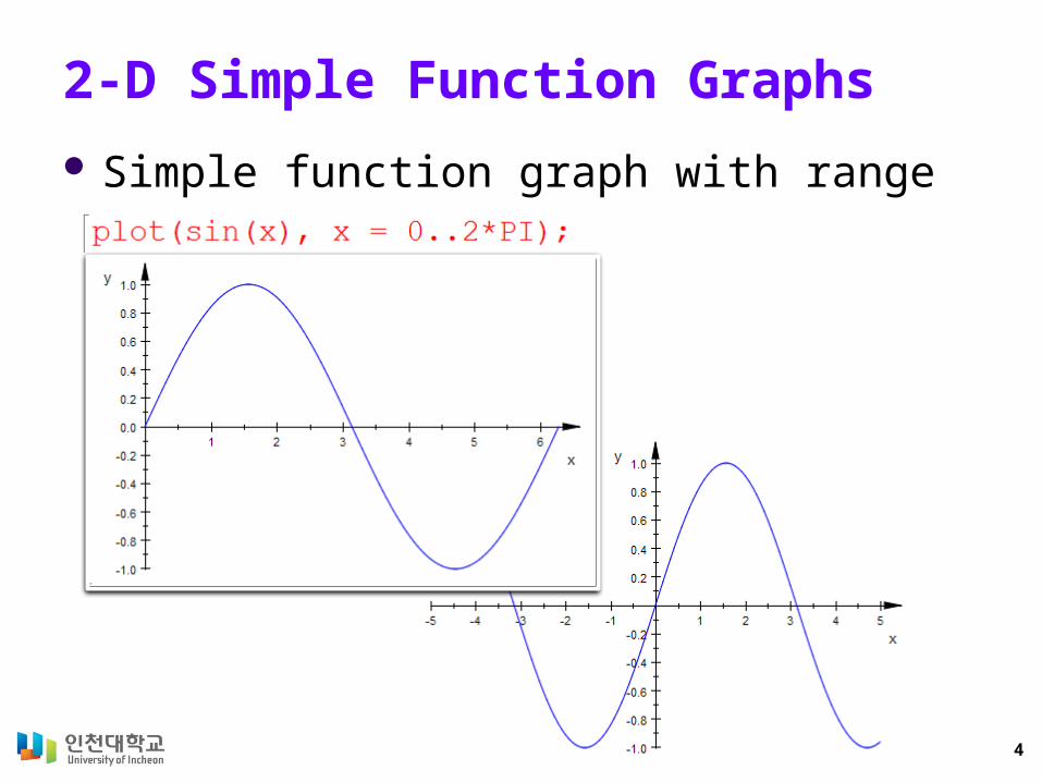
2-D Simple Function Graphs

Simple function graph with range

5

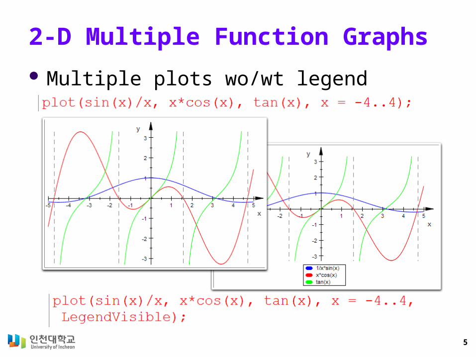
2-D Multiple Function Graphs

Multiple plots wo/wt legend

6

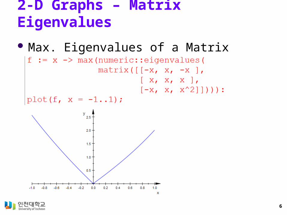
2-D Graphs – Matrix Eigenvalues

Max. Eigenvalues of a Matrix

7

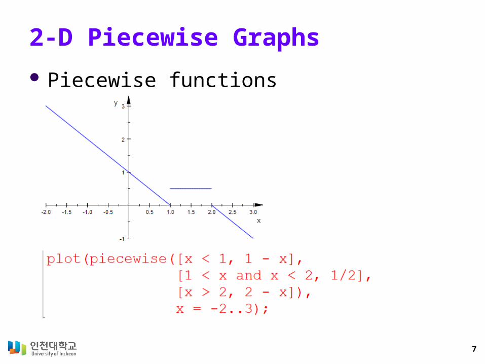
2-D Piecewise Graphs

Piecewise functions

8

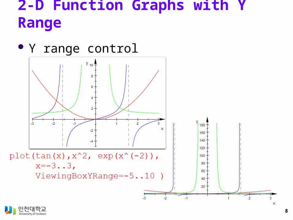
2-D Function Graphs with Y Range

Y range control

9

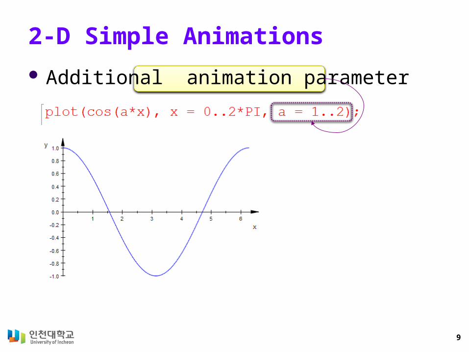
2-D Simple Animations

Additional animation parameter

10

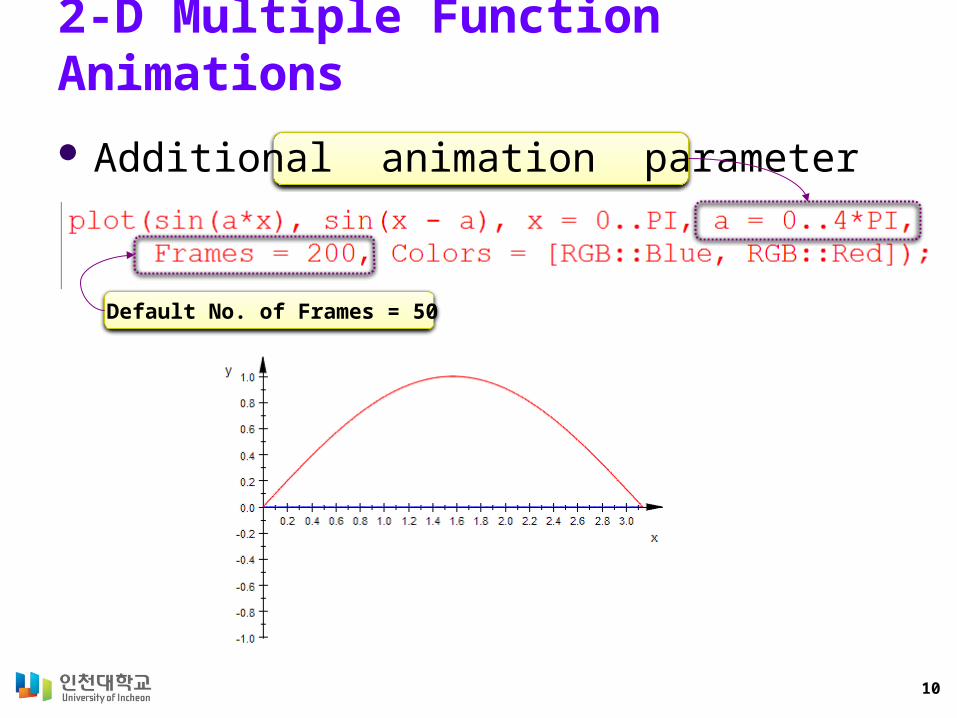
2-D Multiple Function Animations

Additional animation parameter

Default No. of Frames = 50

11

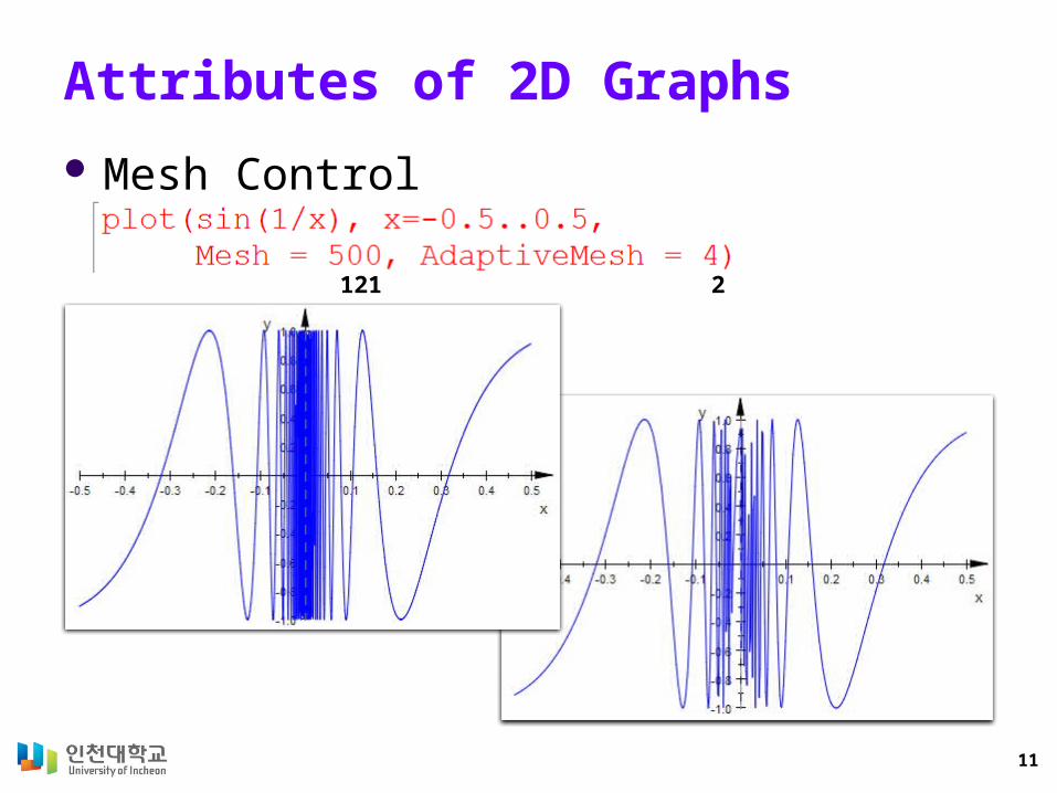
Attributes of 2D Graphs

Mesh Control

121 2

12

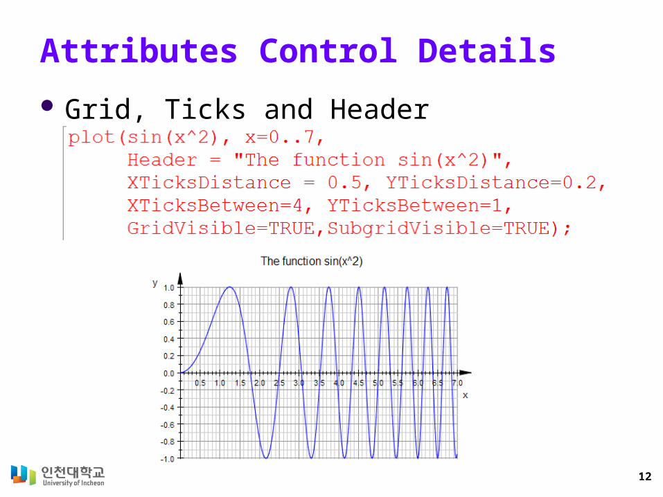
Attributes Control Details

Grid, Ticks and Header

13

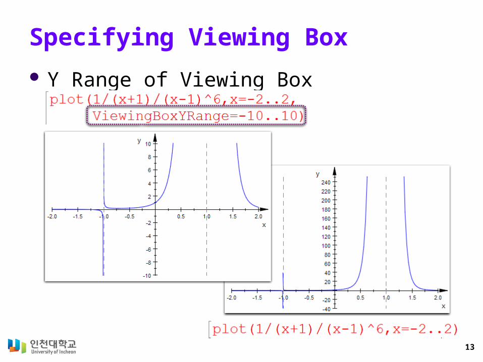
Specifying Viewing Box

Y Range of Viewing Box

14

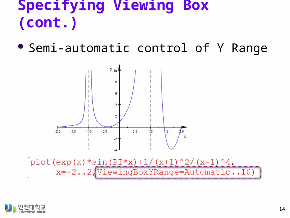
Specifying Viewing Box (cont.)

Semi-automatic control of Y Range

15

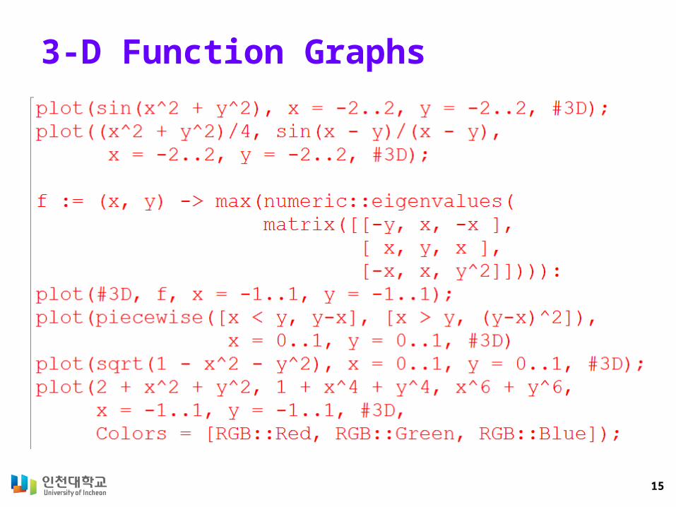
3-D Function Graphs

16

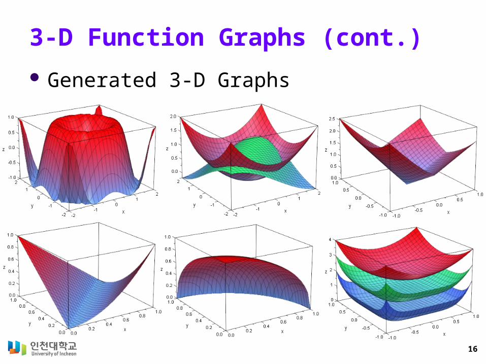
3-D Function Graphs (cont.)

Generated 3-D Graphs

17

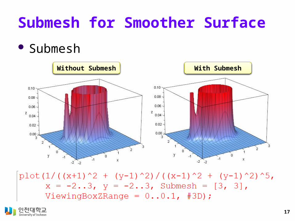
Submesh for Smoother Surface

Submesh

Without Submesh With Submesh

18

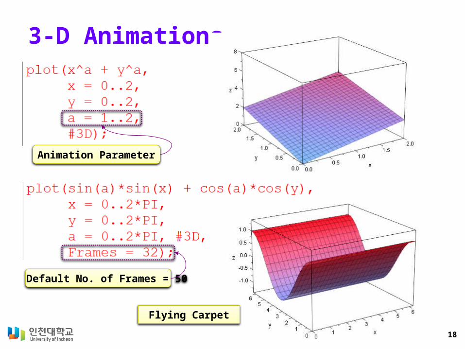
3-D Animations

Default No. of Frames = 50

Animation Parameter

Flying Carpet

19

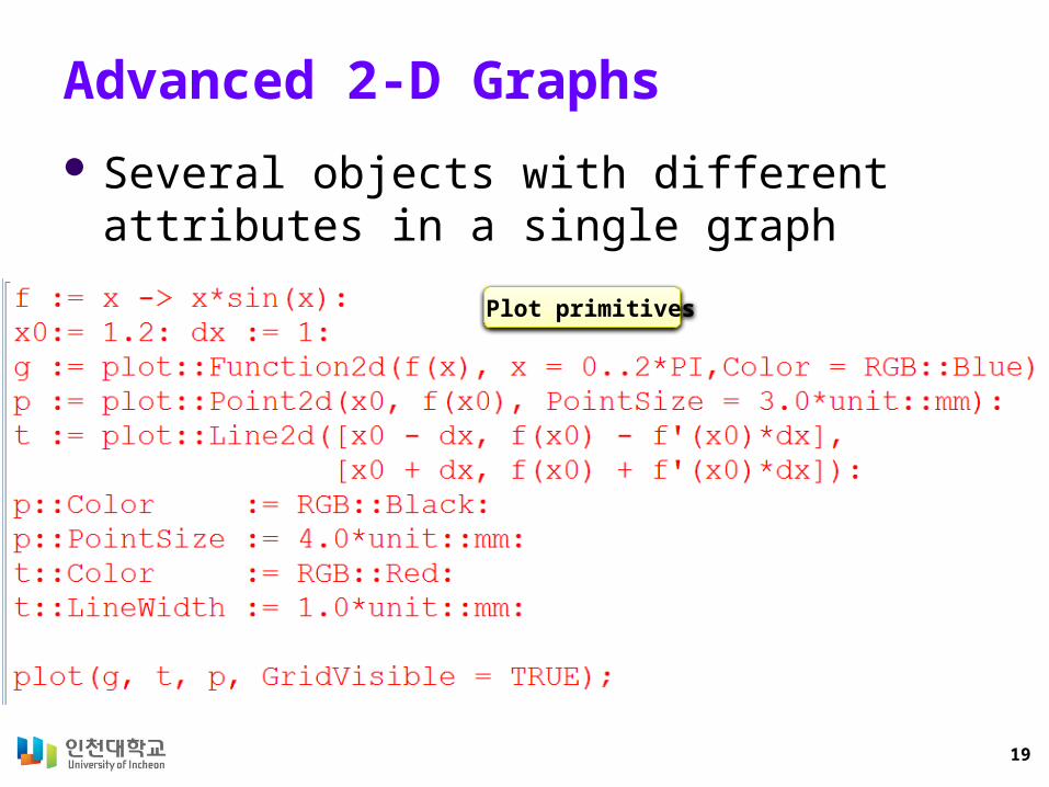
Advanced 2-D Graphs

Several objects with different attributes in a single graph

Plot primitives

20

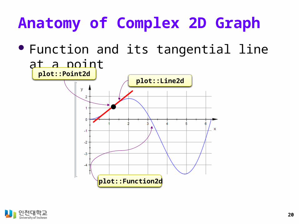
Anatomy of Complex 2D Graph

Function and its tangential line at a point

plot::Point2dplot::Line2d

plot::Function2d

21

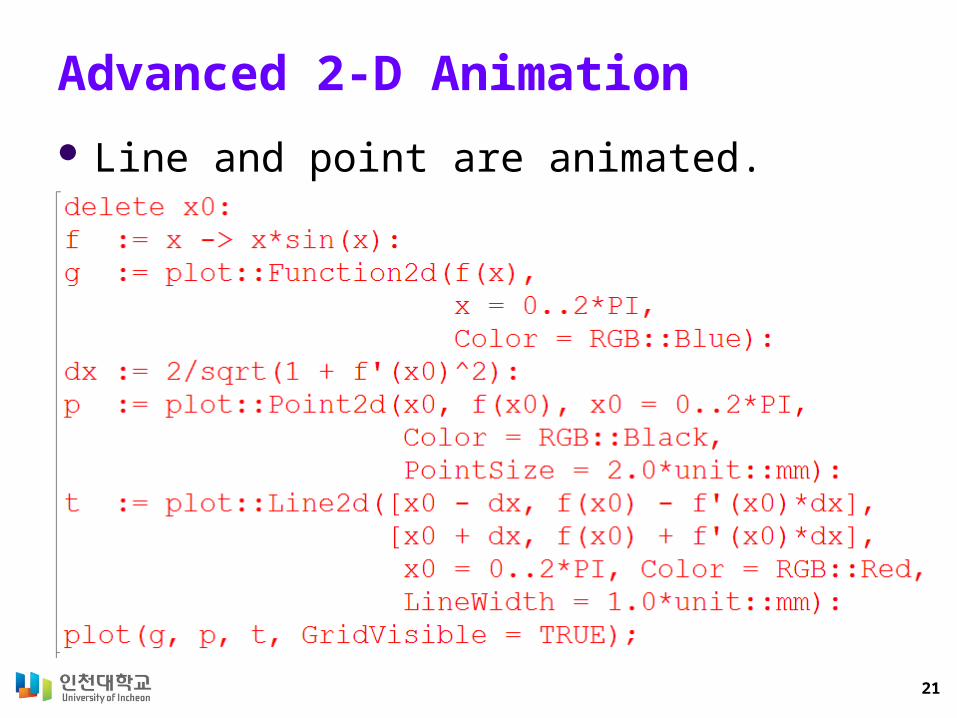
Advanced 2-D Animation

Line and point are animated.

22

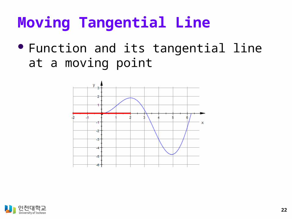
Moving Tangential Line

Function and its tangential line at a moving point

23

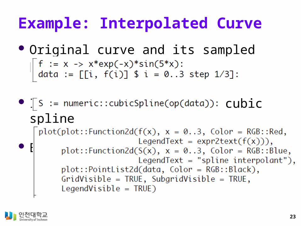
Example: Interpolated Curve

Original curve and its sampled points

Interpolated points using cubic spline

Both curves and sampled points

24

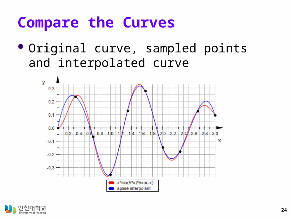
Compare the Curves

Original curve, sampled points and interpo-lated curve

25

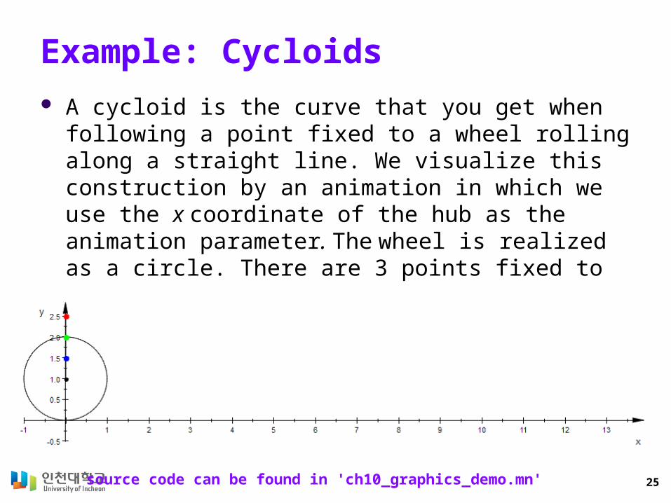
Example: Cycloids A cycloid is the curve that you get when following a point

fixed to a wheel rolling along a straight line. We visualize this construction by an animation in which we use the x coordinate of the hub as the animation parameter. The wheel is realized as a circle. There are 3 points fixed to the wheel: a green point on the rim, a blue point inside the wheel and a red point outside the wheel:

source code can be found in 'ch10_graphics_demo.mn'

26

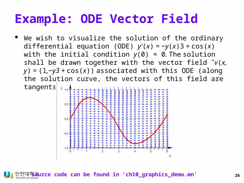
Example: ODE Vector Field We wish to visualize the solution of the ordinary differential equation

(ODE) y′(x) = −y(x)3 + cos(x) with the initial condition y(0) = 0. The so-lution shall be drawn together with the vector field v⃗ (x, y) = (1,−y3 + cos(x)) associated with this ODE (along the solution curve, the vec-tors of this field are tangents of the curve).

source code can be found in 'ch10_graphics_demo.mn'

27

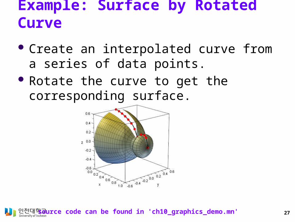
Example: Surface by Rotated Curve

Create an interpolated curve from a series of data points.

Rotate the curve to get the corresponding surface.

source code can be found in 'ch10_graphics_demo.mn'

28

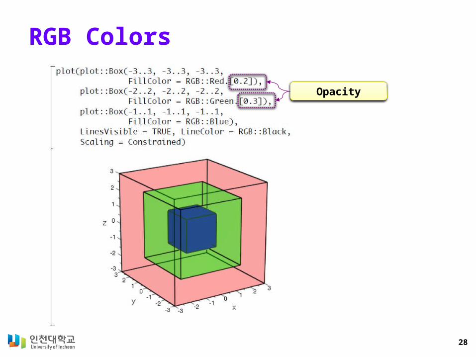
RGB Colors

Opacity

29

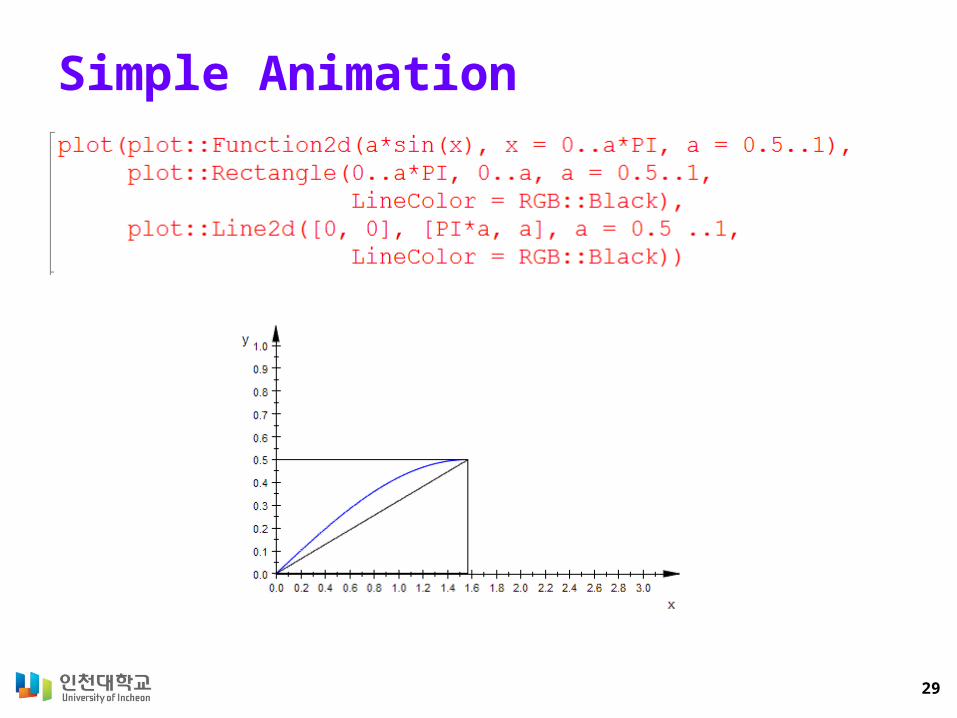
Simple Animation

30

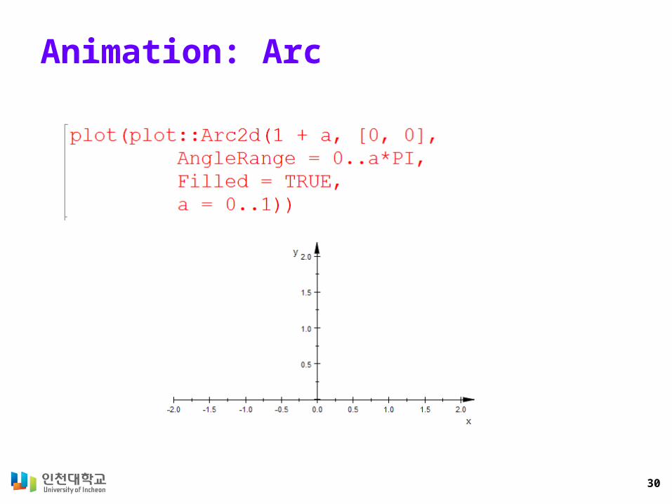
Animation: Arc

31

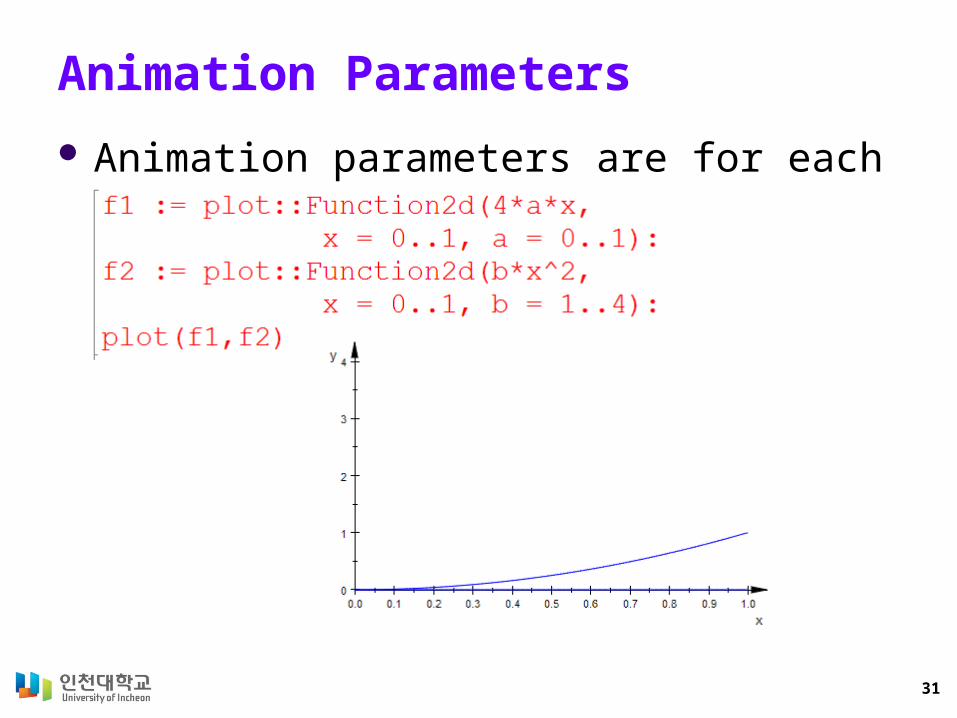
Animation Parameters

Animation parameters are for each objects.

32

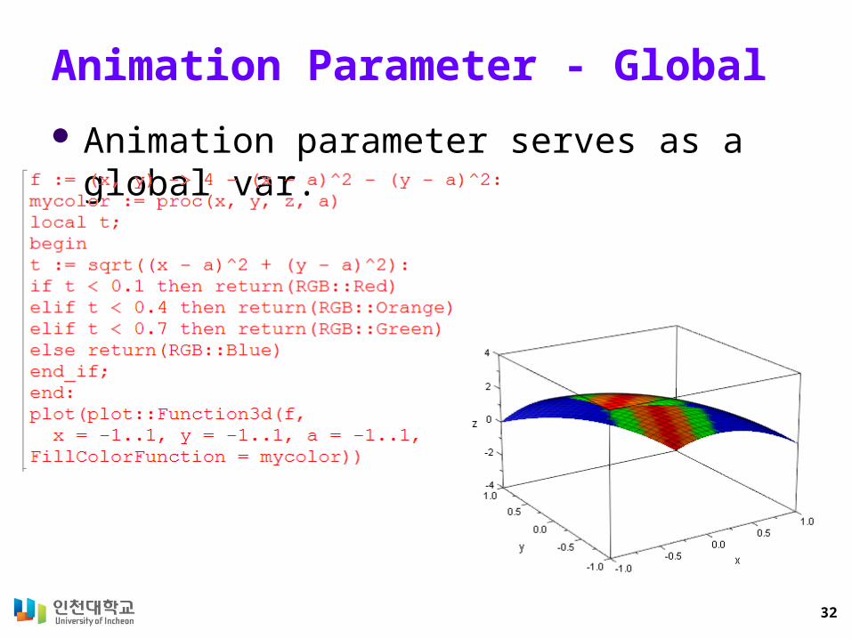
Animation Parameter - Global

Animation parameter serves as a global var.

33

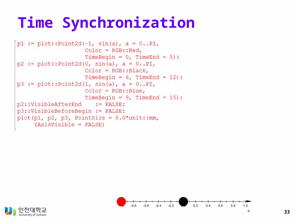
Time Synchronization

34

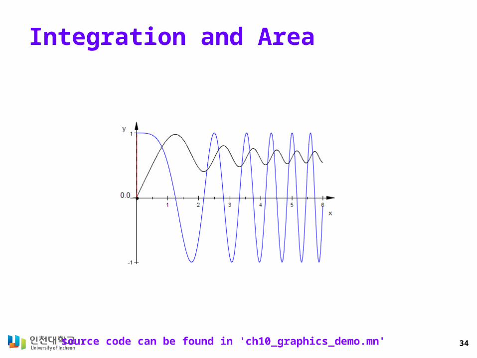
Integration and Area

source code can be found in 'ch10_graphics_demo.mn'

35

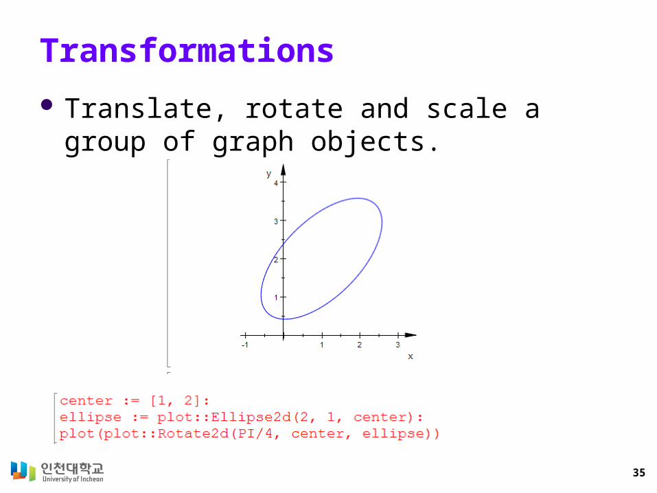
Transformations

Translate, rotate and scale a group of graph objects.

36

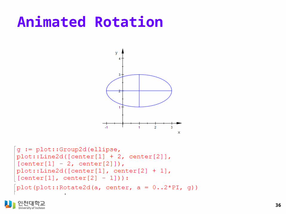
Animated Rotation

37

Using Camera

38

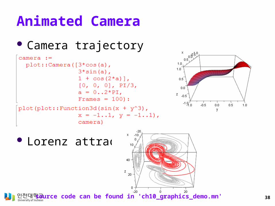
Animated Camera

Camera trajectory

Lorenz attractor

source code can be found in 'ch10_graphics_demo.mn'

39

Key Takeaways

Now, you are able to plot 2-D and 3-D graphs using different objects

and attributes, generate 2-D and 3-D animations with different

objects and attributes, and to control colors and cameras for your

graphs.

40

Notes