CHAPTER 10:

LINEAR DISCRIMINATION

Discriminant-based Classification 3

In classification with K classes (C1,C2,…, Ck)

We defined discriminant function gj(x), j=1,2,…,K

then given any test example x, we chose (predicted) its class label as Ci if gi(x) was the maximum among g1(x), g2(x),…,gk(x)

In previous chapters we have

Used gi(x)=log P(Ci|x)

This is called likelihood classification

Where we used maximum likelihood estimate technique for estimate class likelihood P(x|Ci)

Likelihood- vs. Discriminant-based

Classification 4

Likelihood-based: Assume a model for p(x|Ci), use Bayes’ rule to calculate P(Ci|x)

gi(x) = log P(Ci|x)

This requires estimating class conditional densities P(x|Ci)

For high-dimensional data (many attributes/features), estimating class conditional densities itself is a difficult task

Discriminant-based: Assume a model for gi(x|Φi); no density estimation

Parameters Φi describe the class boundary

Estimating the class boundary is enough for performing classification

no need to accurately estimate the densities inside the boundaries

Linear discriminant:

Advantages:

Simple: O(d) space/computation (d is the number of features)

Knowledge extraction: Weighted sum of attributes;

positive/negative weights, magnitudes (credit scoring)

Optimal when p(x|Ci) are Gaussian with shared cov matrix;

useful when classes are (almost) linearly separable

Linear Discriminant 5

0

1

00 ij

d

jiji

Tiiii wxwwwg

xwwx ,|

Quadratic discriminant:

Higher-order (product) terms:

Map from x to z using nonlinear basis functions and use a linear

discriminant in z-space

Generalized Linear Model 6

215

2

24

2

132211 xxzxzxzxzxz , , , ,

00 iTii

Tiiii wwg xwxxwx WW ,,|

k

jjiji wg

1

xx

Example of non-linear basis functions:

sin(x1)

exp(-(x1-m)2/c)

exp(-||x-m||2/c)

Log(x2)

1(x1>c)

1(ax1+bx2>c)

Generalized Linear Model 7

Two Classes

0

201021

202101

21

w

ww

ww

ggg

T

T

TT

xw

xww

xwxw

xxx

otherwise

if choose

2

1 0

C

gC x

8

Geometry 9

Let the discriminant function is given by g(x)=w1x1+w2x2+w0=

wTx+w0, where w=(w1,w2)T

Take any two points x1, x2, lying on the decision surface

(boundary) g(x)=0

g(x1)=g(x2)=0

wTx1+w0=wTx2+w0 => wT(x1-x2)=0

Note that (x1-x2) is a vector lying on the decision surface

(hyperplane), which means w is normal to any vector lying on the

decision surface

Understanding the geometry 10

Any data point x can be written as a sum of two vectors as

follows

x=xp+r(w/||w||)

xp is normal projection of x on to decision hyper plane (xp lies on the decision hyperplane)

r is distance of x to the hyperplane

g(x)=wTx+w0 =wT(xp+r(w/||w||)+w0=

(wTxp+w0)+r(wTw)/||w||=0+(r||w||2/||w||)=r||w|| => r=g(x)/||w||

Similarly if x=0, r will denote distance of the hyperplane from the origin

g(0)=w0=r||w|| => r=w0/||w||

Understanding the geometry 11

Multiple Classes

00 iTiiii wwg xwwx ,|

xx j

K

ji

i

gg

C

1max

if Choose

12

Classes are

linearly separable

Discriminant function for the ith class is:

During testing, given x, ideally we should have only one gj(x), j=1,2,…,K greater than zero and all others should be less than 0

However, this is not always the case

Positive half spaces of the hyperplane s may overlap

Or we may have all gj(x)<0

These may be taken as “reject” case

Remembering that |gi(x)|/||wi|| is the distance from the input point to the decision hyperplane, assuming all wi have similar length, this assigns point to the class (among all gj(x)>0) to whose decision hyperplane the point is most distant

Multiple classes 13

Pairwise Separation

14

For an input to be assigned to class C1, it should be on the positive side of H12 and H31. We don’t care about the value of H23

It possible that classes are not linearly separable but are pairwise linearly separable

We can use K(K-1)/2 linear discriminants gij(x) to classify

Parameters are computed during training so as to have

Classification is performed as follows

00 ijTijijijij wwg xwwx ,|

otherwisecare tdon'

if

if

j

i

ij C

C

g x

x

x 0

0

0 xij

i

gij

C

,

i f choose

If the class densities are Gaussian, and share a common

covariance matrix, the discriminant function is linear, i.e., when

p (x | Ci ) ~ N ( μi , ∑)

For the special case when there are two classes, we define,

log(y/(1-y) is known as logit transformation or log odds of y

From Discriminants to Posteriors 15

iiTiiii

iTiiii

CPw

wwg

log

,|

μμ2

1μ 1

0

1

00

w

xwwx

otherwise and

log

if choose

| and |

21

21

01

11

50

1

C

yy

yy

y

C

yCPCPy

/

/

.

xx

16

1 1

1

1 2

1 1

2 2

1/2/2 1

1 11

1/2/2 122 2

0

1 1

1 2 0 1 2 1 2

| |logit | log log

1 | |

|log log

|

2 exp 1/ 2 μ μlog log

2 exp 1/ 2 μ μ

1where μ μ μ μ μ μ

2

The inv

d T

d T

T

T

P C P CP C

P C P C

p C P C

p C P C

P C

P C

w

w

x xx

x x

x

x

x x

x x

w x

w

1

0

1

1 0

0

erse of logit is logistic or sigmoid function

|log

1 |

1| sigmoid

1 exp

T

T

T

P Cw

P C

P C ww

xw x

x

x w xw x

In case of two normal classes sharing a common covariance matrix, the log odds is linear

Sigmoid (Logistic) Function 17

50

0

10

10

.

yCwy

gCwgT

T

if choose and sigmoid Calculate

or , if choose and Calculate

xw

xxwx

Logistic Regression 18

Logistic regression is a classification method where in case of

binary classification, the log ratio of p(C1|x) and p(C2|x) is

modeled as a linear function

Since we are modeling ratio of posterior probability directly, there is

no need for density estimation i.e. p(x|C1) and p(x|C2)

Note that this is slightly different version than what is given in the book

but this is the most widely version in practice

Rearranging, we can write

Given x, predicted label is C1 when P(C1|x)>P(C2|x)

Or alternatively, when, wTx+w0>0

To classify using this model, that we need to know what w and w0 is

How do we find w and w0?

1

1 0

2

|logit | log

| |

Tp C

P C wp C

x

x w xx

0

1 2

0 0

exp1| and |

1 exp 1 exp

T

T T

wP C P C

w w

w xx x

w x w x

Logistic Regression for binary classification

19

Given training data rt|xt is modeled as Bernoulli

distribution

To estimate w and w0, we can

Maximize the likelihood

Or, equivalently maximize the log-likelihood

Or equivalently, minimize negative log-likelihood

1

,N

t t

tr

xX

1

0

1| ~ Bernoulli where, |

1 exp

t t t t t

T tr y y P C

w

x xw x

1

0, | 1t tr r

t t

t

l w y y

w X

0, | log 1 log 1t t t t

t

L w r y r y w X

0 0, | , | log 1 log 1t t t t

t

E w L w r y r y w wX X

Gradient-Descent 20

T

d

ww

E

w

E

w

EE

,...,,

21

E(w|X) is error with parameters w on sample X

w*=arg minw E(w | X)

Gradient

Gradient-descent: Starts from random w and updates w iteratively in the

negative direction of gradient

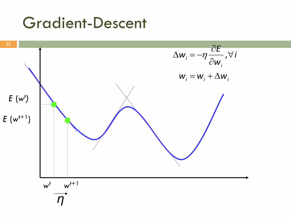
Gradient-Descent 21

iii

i

i

www

iw

Ew

,

wt wt+1

η

E (wt)

E (wt+1)

Gradient-Descent 22

Gradient-Descent 23

Training: Gradient-Descent 24

t

tt

t

tj

tt

tj

tt

tt

t

t

t

j

j

ttt

t

t

yrw

Ew

djxyr

xyyy

r

y

r

w

Ew

yyda

dyy

yryrwE

0

0

0

1

11

1

1

11

,...,,

,

asigmoid If

log log|Xw

25

26

10

100 1000

Logistic Regression for K classes (K>2) 27

Given training data rt|xt is modeled as Multinomial distribution

To estimate w1, w2,…,wK and w10,w20,…,wK0 we can

Maximize the likelihood

Or equivalently, minimize negative log-likelihood

The gradient can computed using simple formula

Using gradient descent, we can have simple algorithm for logistic regresison for K class classification problem

1

,N

t t

tr

xX

0 t t t t t

j j j j j j

t t

r y w r y w x

0

01

exp| ~ Mult 1, where, | , 1,...,

exp

T t

i it t t t

K i i K T t

j jj

wr y P C i K

w

w xx y x

w x

0 1, |

tirK t

i i iit i

l w y

w X

0 1, | log

K t t

i i i iit

E w r y

w X

This is known as

softmax function

28