Chapter 10

Standard Costs and the Balanced Scorecard

10-2

Standard Costs

Standards are benchmarks or “norms”for measuring performance. Two types

of standards are commonly used.

Quantity standardsspecify how much of aninput should be used to

make a product orprovide a service.

Cost (price)standards specify

how much should be paid for each unit

of the input.

10-3

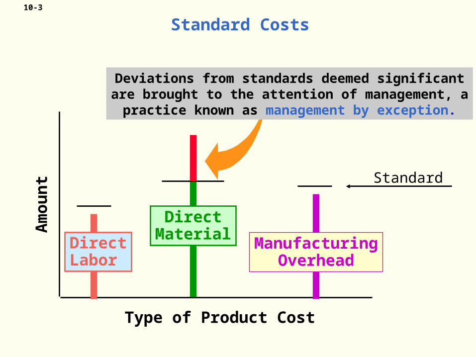
Standard Costs

DirectMaterial

Deviations from standards deemed significantare brought to the attention of management, apractice known as management by exception.

Type of Product Cost

Am

ou

nt

DirectLabor

ManufacturingOverhead

Standard

10-4

Variance Analysis Cycle

Prepare standard cost

performance report

Analyze variances

Begin

Identifyquestions

Receive explanations

Takecorrective

actions

Conduct next period’s

operations

Exhibit10-1

10-5

Accountants, engineers, purchasingagents, and production managers

combine efforts to set standards that encourage efficient future production.

Setting Standard Costs

10-6

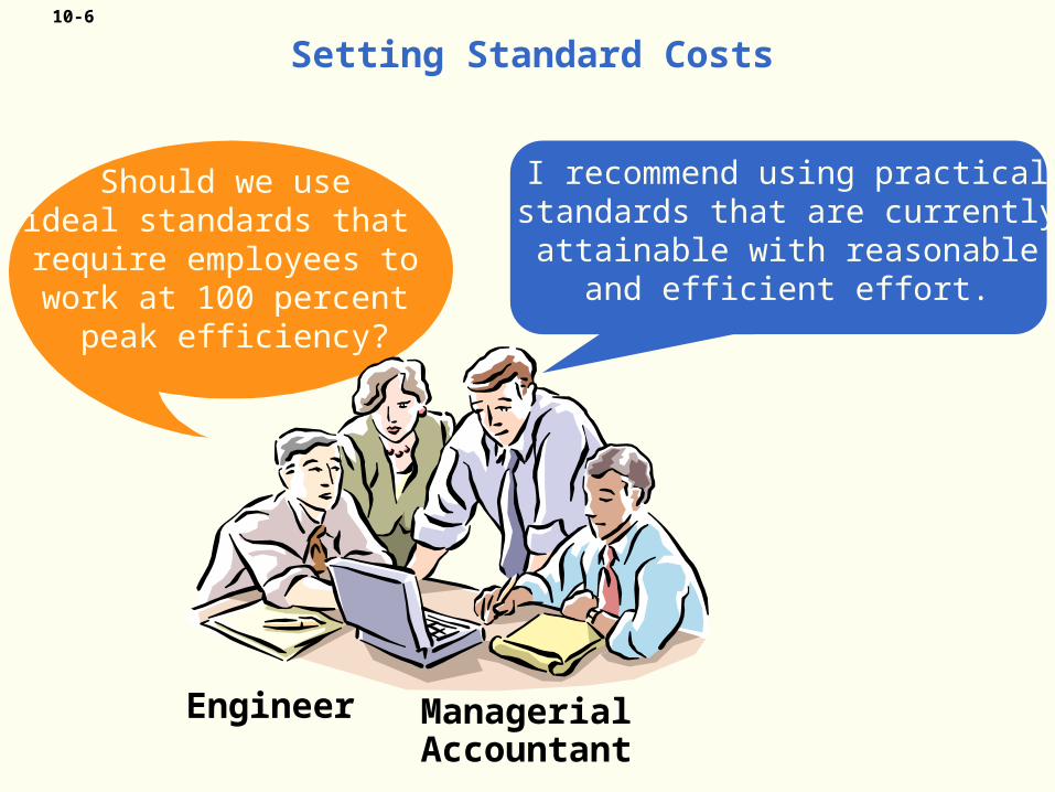
Setting Standard Costs

Should we useideal standards that require employees towork at 100 percent

peak efficiency?

Engineer ManagerialAccountant

I recommend using practical standards that are currently

attainable with reasonable and efficient effort.

10-7

Learning Objective 1

Explain how direct materials standards

and direct laborstandards are set.

10-8

Setting Direct Material Standards

PriceStandards

Summarized in a Bill of Materials.

Final, deliveredcost of materials,net of discounts.

QuantityStandards

10-9

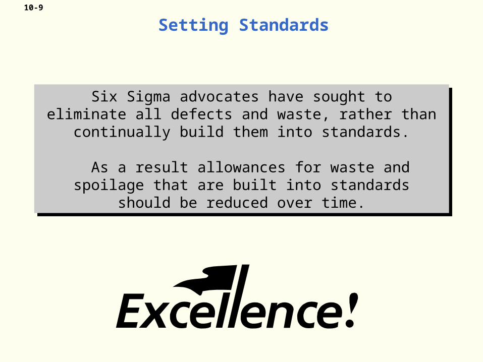
Setting Standards

Six Sigma advocates have sought toeliminate all defects and waste, rather than

continually build them into standards.

As a result allowances for waste andspoilage that are built into standards

should be reduced over time.

Six Sigma advocates have sought toeliminate all defects and waste, rather than

continually build them into standards.

As a result allowances for waste andspoilage that are built into standards

should be reduced over time.

10-10

Setting Direct Labor Standards

RateStandards

Often a singlerate is used that reflectsthe mix of wages earned.

TimeStandards

Use time and motion studies for

each labor operation.

10-11

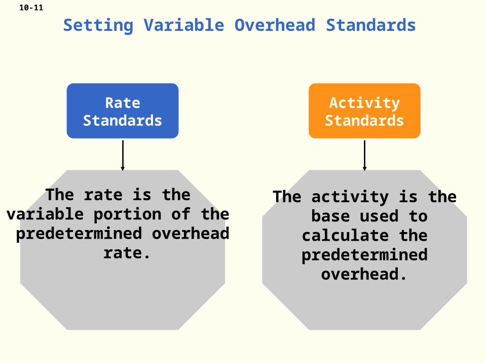
Setting Variable Overhead Standards

RateStandards

The rate is the variable portion of the

predetermined overhead rate.

ActivityStandards

The activity is the base used to calculate

the predetermined overhead.

10-12

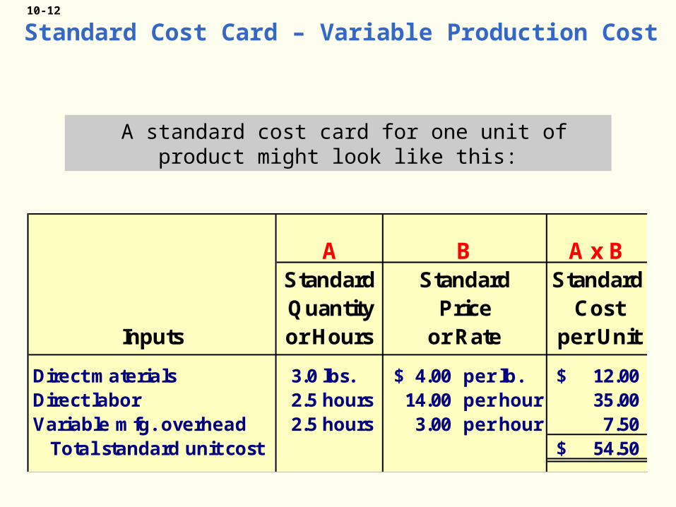
Standard Cost Card – Variable Production Cost

A standard cost card for one unit of product might look like this:

A A x BStandard Standard StandardQuantity Price Cost

Inputs or Hours or Rate per Unit

Direct materials 3.0 lbs. 4.00$ per lb. 12.00$ Direct labor 2.5 hours 14.00 per hour 35.00 Variable mfg. overhead 2.5 hours 3.00 per hour 7.50 Total standard unit cost 54.50$

B

10-13

Are standards the same as budgets? A budget is set for

total costs.

Standards vs. Budgets

A standard is a per unit cost.Standards are

often used when preparing budgets.

10-14

Price and Quantity Standards

Price and and quantity standards are determined separately for two reasons:

The purchasing manager is responsible for raw material purchase prices and the production manager is responsible for the quantity of raw material used.

The purchasing manager is responsible for raw material purchase prices and the production manager is responsible for the quantity of raw material used.

The buying and using activities occur at different times. Raw material purchases may be held in inventory for a period of time before being used in production.

The buying and using activities occur at different times. Raw material purchases may be held in inventory for a period of time before being used in production.

10-15

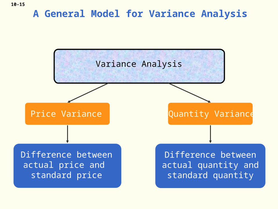
A General Model for Variance Analysis

Variance Analysis

Price Variance

Difference betweenactual price and standard price

Quantity Variance

Difference betweenactual quantity andstandard quantity

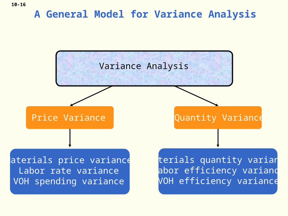
10-16

Variance Analysis

Price Variance Quantity Variance

Materials price varianceLabor rate variance

VOH spending variance

Materials quantity varianceLabor efficiency varianceVOH efficiency variance

A General Model for Variance Analysis

10-17

Price Variance Quantity Variance

Actual Quantity Actual Quantity Standard Quantity × - × - × Actual Price Standard Price Standard Price

A General Model for Variance Analysis

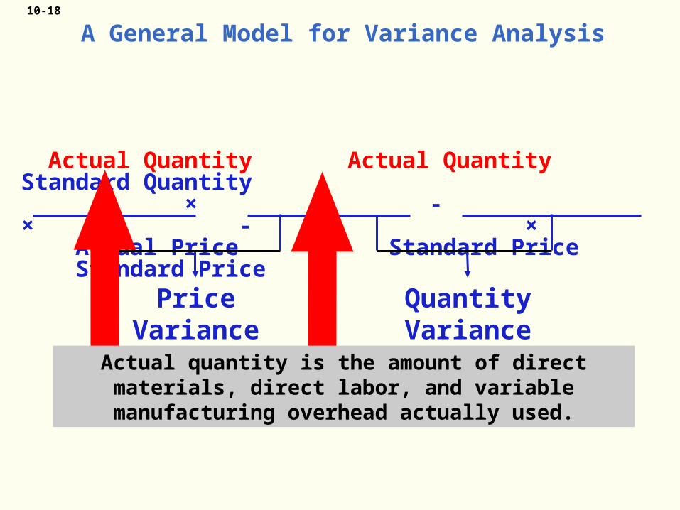
10-18

Price Variance Quantity Variance

Actual Quantity Actual Quantity Standard Quantity × - × - × Actual Price Standard Price Standard Price

A General Model for Variance Analysis

Actual quantity is the amount of direct materials, direct labor, and variable

manufacturing overhead actually used.

10-19

Price Variance Quantity Variance

Actual Quantity Actual Quantity Standard Quantity × - × - × Actual Price Standard Price Standard Price

A General Model for Variance Analysis

Standard quantity is the standard quantity allowed for the actual output of the period.

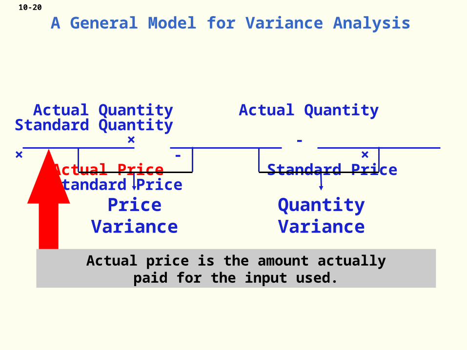
10-20

Price Variance Quantity Variance

Actual Quantity Actual Quantity Standard Quantity × - × - × Actual Price Standard Price Standard Price

A General Model for Variance Analysis

Actual price is the amount actuallypaid for the input used.

10-21

A General Model for Variance Analysis

Standard price is the amount that should have been paid for the input used.

Price Variance Quantity Variance

Actual Quantity Actual Quantity Standard Quantity × - × - × Actual Price Standard Price Standard Price

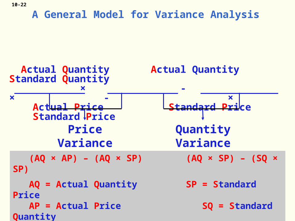
10-22

A General Model for Variance Analysis

(AQ × AP) – (AQ × SP) (AQ × SP) – (SQ × SP)

AQ = Actual Quantity SP = Standard Price AP = Actual Price SQ = Standard Quantity

Price Variance Quantity Variance

Actual Quantity Actual Quantity Standard Quantity × - × - × Actual Price Standard Price Standard Price

10-23

Learning Objective 2

Compute the direct materials price and

quantity variances and explain their significance.

10-24

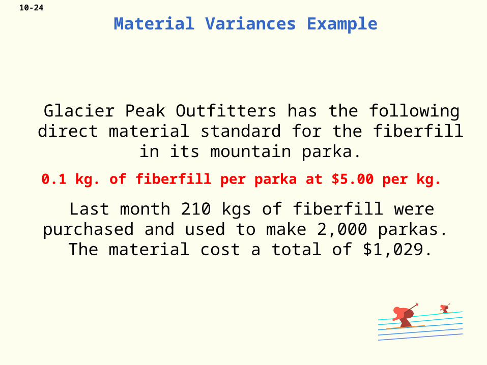
Glacier Peak Outfitters has the following direct material standard for the fiberfill in its mountain

parka.

0.1 kg. of fiberfill per parka at $5.00 per kg.

Last month 210 kgs of fiberfill were purchased and used to make 2,000 parkas. The material cost a

total of $1,029.

Material Variances Example

10-25

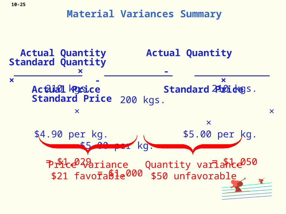
210 kgs. 210 kgs. 200 kgs. × × × $4.90 per kg. $5.00 per kg. $5.00 per kg.

= $1,029 = $1,050 = $1,000

Price variance$21 favorable

Quantity variance$50 unfavorable

Actual Quantity Actual Quantity Standard Quantity × - × - × Actual Price Standard Price Standard Price

Material Variances Summary

10-26

210 kgs. 210 kgs. 200 kgs. × × × $4.90 per kg. $5.00 per kg. $5.00 per kg.

= $1,029 = $1,050 = $1,000

Price variance$21 favorable

Quantity variance$50 unfavorable

Actual Quantity Actual Quantity Standard Quantity × - × - × Actual Price Standard Price Standard Price

$1,029 210 kgs = $4.90 per kg

Material Variances Summary

10-27

210 kgs. 210 kgs. 200 kgs. × × × $4.90 per kg. $5.00 per kg. $5.00 per kg.

= $1,029 = $1,050 = $1,000

Price variance$21 favorable

Quantity variance$50 unfavorable

Actual Quantity Actual Quantity Standard Quantity × - × - × Actual Price Standard Price Standard Price

0.1 kg per parka 2,000 parkas = 200 kgs

Material Variances Summary

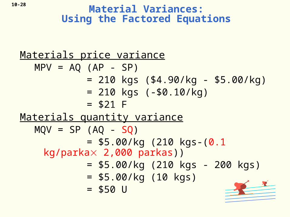
10-28Material Variances:

Using the Factored Equations

Materials price varianceMPV = AQ (AP - SP) = 210 kgs ($4.90/kg - $5.00/kg) = 210 kgs (-$0.10/kg) = $21 F

Materials quantity varianceMQV = SP (AQ - SQ) = $5.00/kg (210 kgs-(0.1 kg/parka 2,000

parkas)) = $5.00/kg (210 kgs - 200 kgs) = $5.00/kg (10 kgs) = $50 U

10-29

Isolation of Material Variances

I need the price variancesooner so that I can better

identify purchasing problems.

You accountants just don’tunderstand the problems thatpurchasing managers have.

I’ll start computingthe price variancewhen material is

purchased rather thanwhen it’s used.

10-30

Material Variances

Hanson purchased and used 1,700 pounds. How

are the variances computed if the amount purchased differs from

the amount used?

The price variance is computed on the entire

quantity purchased.

The quantity variance is computed only on the

quantity used.

10-31

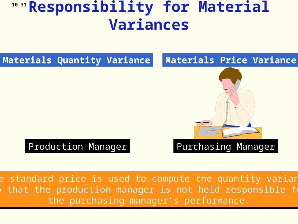
Responsibility for Material Variances

Materials Price VarianceMaterials Quantity Variance

Production Manager Purchasing Manager

The standard price is used to compute the quantity varianceso that the production manager is not held responsible for

the purchasing manager’s performance.

The standard price is used to compute the quantity varianceso that the production manager is not held responsible for

the purchasing manager’s performance.

10-32

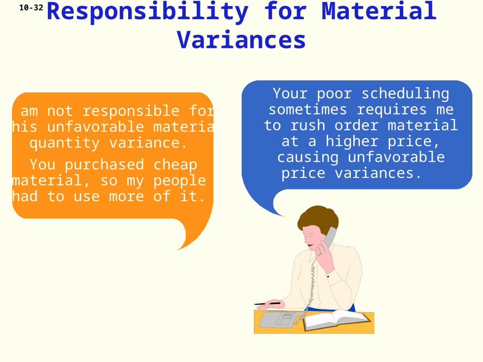
I am not responsible for this unfavorable material

quantity variance.

You purchased cheapmaterial, so my peoplehad to use more of it.

Your poor scheduling sometimes requires me to rush order material at a

higher price, causing unfavorable price variances.

Responsibility for Material Variances

10-33

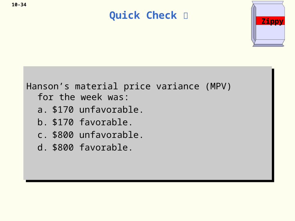
Hanson Inc. has the following direct material standard to manufacture one Zippy:

1.5 pounds per Zippy at $4.00 per pound

Last week, 1,700 pounds of material were purchased and used to make 1,000 Zippies. The material cost a total of

$6,630.

ZippyQuick Check

10-34

Quick Check Zippy

Hanson’s material price variance (MPV)

for the week was:a. $170 unfavorable.b. $170 favorable.c. $800 unfavorable.d. $800 favorable.

Hanson’s material price variance (MPV)

for the week was:a. $170 unfavorable.b. $170 favorable.c. $800 unfavorable.d. $800 favorable.

10-35

Hanson’s material price variance (MPV)

for the week was:a. $170 unfavorable.b. $170 favorable.c. $800 unfavorable.d. $800 favorable.

Hanson’s material price variance (MPV)

for the week was:a. $170 unfavorable.b. $170 favorable.c. $800 unfavorable.d. $800 favorable. MPV = AQ(AP - SP)

MPV = 1,700 lbs. × ($3.90 - 4.00) MPV = $170 Favorable

Quick Check Zippy

10-36

Quick Check

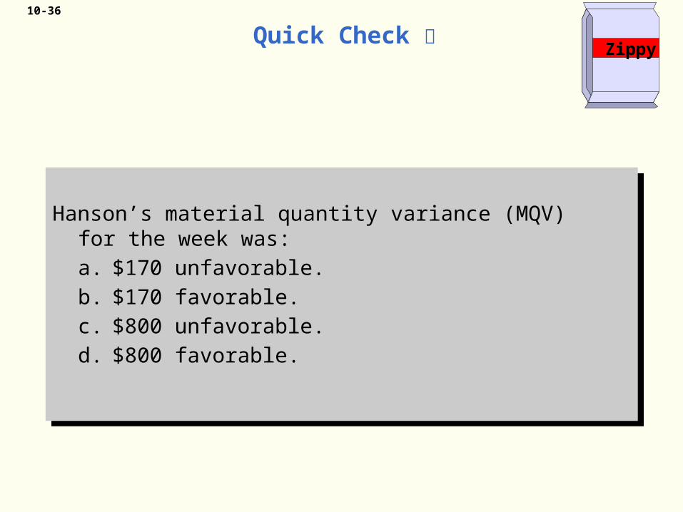
Hanson’s material quantity variance (MQV)

for the week was:a. $170 unfavorable.b. $170 favorable.c. $800 unfavorable.d. $800 favorable.

Hanson’s material quantity variance (MQV)

for the week was:a. $170 unfavorable.b. $170 favorable.c. $800 unfavorable.d. $800 favorable.

Zippy

10-37

Hanson’s material quantity variance (MQV)

for the week was:a. $170 unfavorable.b. $170 favorable.c. $800 unfavorable.d. $800 favorable.

Hanson’s material quantity variance (MQV)

for the week was:a. $170 unfavorable.b. $170 favorable.c. $800 unfavorable.d. $800 favorable.

MQV = SP(AQ - SQ) MQV = $4.00(1,700 lbs - 1,500 lbs) MQV = $800 unfavorable

Quick Check Zippy

10-38

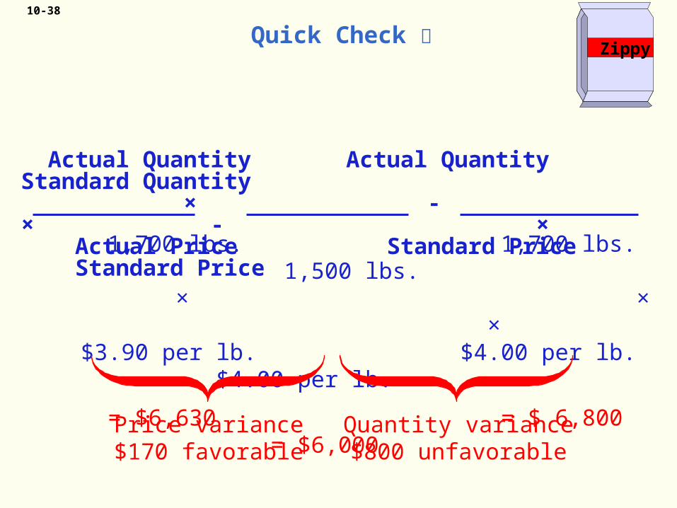
1,700 lbs. 1,700 lbs. 1,500 lbs. × × × $3.90 per lb. $4.00 per lb. $4.00 per lb.

= $6,630 = $ 6,800 = $6,000

Price variance$170 favorable

Quantity variance$800 unfavorable

Actual Quantity Actual Quantity Standard Quantity × - × - × Actual Price Standard Price Standard Price

ZippyQuick Check

10-39

Hanson Inc. has the following material standard to manufacture one Zippy:

1.5 pounds per Zippy at $4.00 per pound

Last week, 2,800 pounds of material were purchased at a total cost of $10,920, and 1,700 pounds were used to

make 1,000 Zippies.

ZippyQuick Check Continued

10-40

Actual Quantity Actual Quantity Purchased Purchased × - × Actual Price Standard Price 2,800 lbs. 2,800 lbs. × × $3.90 per lb. $4.00 per lb.

= $10,920 = $11,200

Price variance$280 favorable

Price variance increases because quantity

purchased increases.

ZippyQuick Check Continued

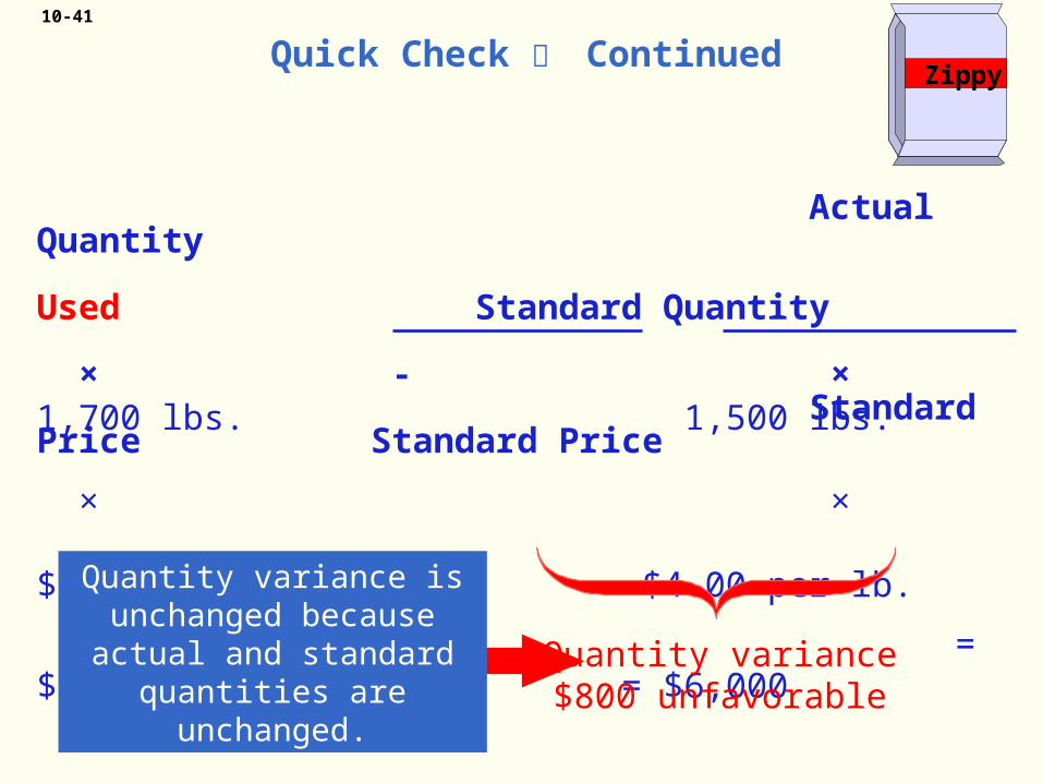
10-41

Actual Quantity Used Standard Quantity × - × Standard Price Standard Price 1,700 lbs. 1,500 lbs. × × $4.00 per lb. $4.00 per lb.

= $6,800 = $6,000

Quantity variance$800 unfavorable

Quantity variance is unchanged because actual and standard

quantities are unchanged.

ZippyQuick Check Continued

10-42

Learning Objective 3

Compute the direct labor rate and

efficiency variances and explain

their significance.

10-43

Glacier Peak Outfitters has the following direct labor standard for its mountain parka.

1.2 standard hours per parka at $10.00 per hour

Last month, employees actually worked 2,500 hours at a total labor cost of $26,250 to make 2,000 parkas.

Labor Variances Example

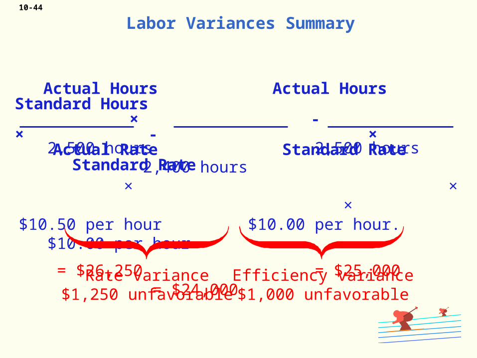
10-44

2,500 hours 2,500 hours 2,400 hours × × ×$10.50 per hour $10.00 per hour. $10.00 per hour

= $26,250 = $25,000 = $24,000

Rate variance$1,250 unfavorable

Efficiency variance$1,000 unfavorable

Actual Hours Actual Hours Standard Hours × - × - × Actual Rate Standard Rate Standard Rate

Labor Variances Summary

10-45

Labor Variances Summary

2,500 hours 2,500 hours 2,400 hours × × ×$10.50 per hour $10.00 per hour. $10.00 per hour

= $26,250 = $25,000 = $24,000

Actual Hours Actual Hours Standard Hours × - × - × Actual Rate Standard Rate Standard Rate

$26,250 2,500 hours = $10.50 per hour

Rate variance$1,250 unfavorable

Efficiency variance$1,000 unfavorable

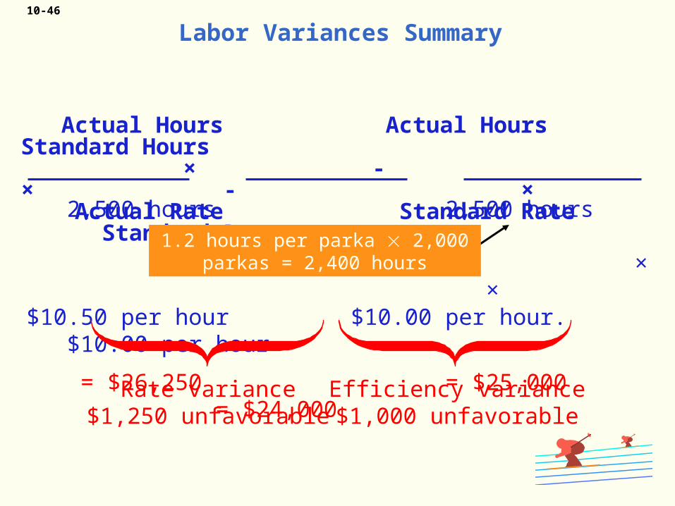
10-46

Labor Variances Summary

2,500 hours 2,500 hours 2,400 hours × × ×$10.50 per hour $10.00 per hour. $10.00 per hour

= $26,250 = $25,000 = $24,000

Actual Hours Actual Hours Standard Hours × - × - × Actual Rate Standard Rate Standard Rate

1.2 hours per parka 2,000 parkas = 2,400 hours

Rate variance$1,250 unfavorable

Efficiency variance$1,000 unfavorable

10-47Labor Variances:

Using the Factored Equations

Labor rate varianceLRV = AH (AR - SR) = 2,500 hours ($10.50 per hour – $10.00 per

hour) = 2,500 hours ($0.50 per hour) = $1,250 unfavorable

Labor efficiency varianceLEV = SR (AH - SH) = $10.00 per hour (2,500 hours – 2,400 hours) = $10.00 per hour (100 hours) = $1,000 unfavorable

10-48

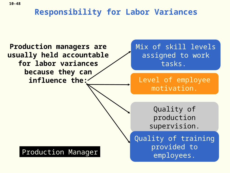
Responsibility for Labor Variances

Production Manager

Production managers areusually held accountable

for labor variancesbecause they can

influence the:

Mix of skill levelsassigned to work

tasks.

Level of employee motivation.

Quality of production supervision.

Quality of training provided to employees.

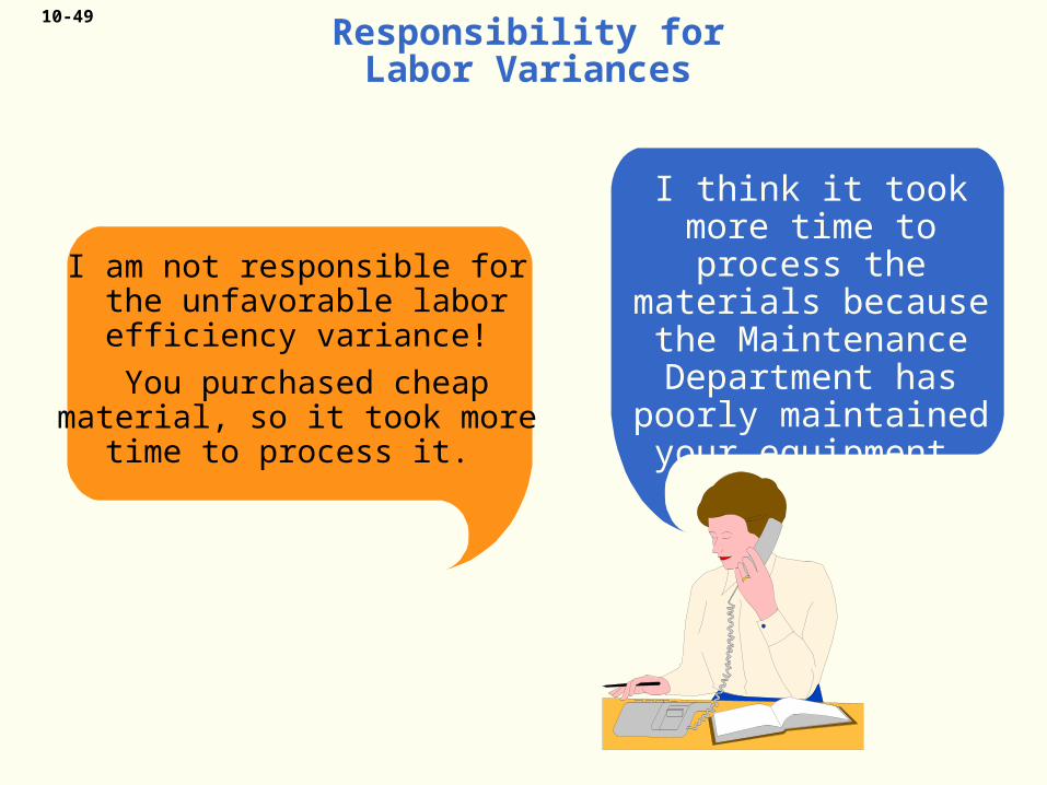
10-49Responsibility forLabor Variances

I am not responsible for the unfavorable labor

efficiency variance!

You purchased cheapmaterial, so it took more

time to process it.

I think it took more time to process the

materials because the Maintenance

Department has poorly maintained your

equipment.

10-50

Hanson Inc. has the following direct labor standard to manufacture one Zippy:

1.5 standard hours per Zippy at $12.00 perdirect labor hour

Last week, 1,550 direct labor hours were worked at a total labor cost of $18,910

to make 1,000 Zippies.

ZippyQuick Check

10-51

Hanson’s labor rate variance (LRV) for the week

was:a. $310 unfavorable.b. $310 favorable.c. $300 unfavorable.d. $300 favorable.

Hanson’s labor rate variance (LRV) for the week

was:a. $310 unfavorable.b. $310 favorable.c. $300 unfavorable.d. $300 favorable.

Quick Check Zippy

10-52

Hanson’s labor rate variance (LRV) for the week

was:a. $310 unfavorable.b. $310 favorable.c. $300 unfavorable.d. $300 favorable.

Hanson’s labor rate variance (LRV) for the week

was:a. $310 unfavorable.b. $310 favorable.c. $300 unfavorable.d. $300 favorable.

Quick Check

LRV = AH(AR - SR) LRV = 1,550 hrs($12.20 - $12.00) LRV = $310 unfavorable

Zippy

10-53

Hanson’s labor efficiency variance (LEV)

for the week was:a. $590 unfavorable.b. $590 favorable.c. $600 unfavorable.d. $600 favorable.

Hanson’s labor efficiency variance (LEV)

for the week was:a. $590 unfavorable.b. $590 favorable.c. $600 unfavorable.d. $600 favorable.

Quick Check Zippy

10-54

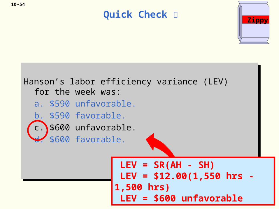
Hanson’s labor efficiency variance (LEV)

for the week was:a. $590 unfavorable.b. $590 favorable.c. $600 unfavorable.d. $600 favorable.

Hanson’s labor efficiency variance (LEV)

for the week was:a. $590 unfavorable.b. $590 favorable.c. $600 unfavorable.d. $600 favorable.

Quick Check

LEV = SR(AH - SH) LEV = $12.00(1,550 hrs - 1,500 hrs) LEV = $600 unfavorable

Zippy

10-55

Actual Hours Actual Hours Standard Hours × - × - × Actual Rate Standard Rate Standard Rate

Rate variance$310 unfavorable

Efficiency variance$600 unfavorable

1,550 hours 1,550 hours 1,500 hours × × × $12.20 per hour $12.00 per hour $12.00 per hour

= $18,910 = $18,600 = $18,000

ZippyQuick Check

10-56

Learning Objective 4

Compute the variable manufacturing

overhead spending and efficiency variances.

10-57

Glacier Peak Outfitters has the following direct variable manufacturing overhead labor standard for its mountain

parka.

1.2 standard hours per parka at $4.00 per hour

Last month, employees actually worked 2,500 hours to make 2,000 parkas. Actual variable manufacturing

overhead for the month was $10,500.

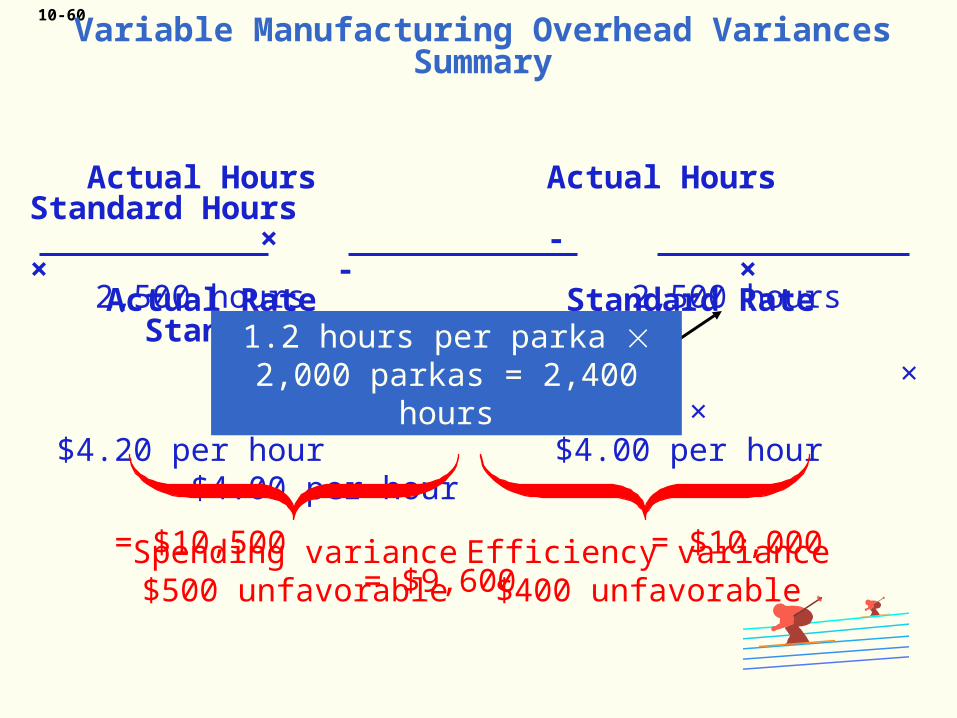
Variable Manufacturing Overhead Variances Example

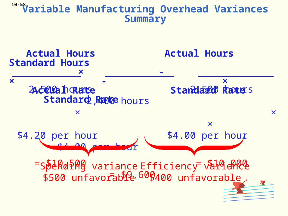
10-58

2,500 hours 2,500 hours 2,400 hours × × × $4.20 per hour $4.00 per hour $4.00 per hour

= $10,500 = $10,000 = $9,600

Spending variance$500 unfavorable

Efficiency variance$400 unfavorable

Actual Hours Actual Hours Standard Hours × - × - × Actual Rate Standard Rate Standard Rate

Variable Manufacturing Overhead Variances Summary

10-59

Actual Hours Actual Hours Standard Hours × - × - × Actual Rate Standard Rate Standard Rate

2,500 hours 2,500 hours 2,400 hours × × × $4.20 per hour $4.00 per hour $4.00 per hour

= $10,500 = $10,000 = $9,600

Spending variance$500 unfavorable

Efficiency variance$400 unfavorable

$10,500 2,500 hours = $4.20 per hour

Variable Manufacturing Overhead Variances Summary

10-60

Actual Hours Actual Hours Standard Hours × - × - × Actual Rate Standard Rate Standard Rate

2,500 hours 2,500 hours 2,400 hours × × × $4.20 per hour $4.00 per hour $4.00 per hour

= $10,500 = $10,000 = $9,600

Spending variance$500 unfavorable

Efficiency variance$400 unfavorable

1.2 hours per parka 2,000 parkas = 2,400 hours

Variable Manufacturing Overhead Variances Summary

10-61Variable Manufacturing Overhead Variances:

Using Factored Equations

Variable manufacturing overhead spending varianceVMSV = AH (AR - SR) = 2,500 hours ($4.20 per hour – $4.00 per

hour) = 2,500 hours ($0.20 per hour) = $500 unfavorable

Variable manufacturing overhead efficiency varianceVMEV = SR (AH - SH) = $4.00 per hour (2,500 hours – 2,400 hours) = $4.00 per hour (100 hours) = $400 unfavorable

10-62

Hanson Inc. has the following variable manufacturing overhead standard to

manufacture one Zippy:

1.5 standard hours per Zippy at $3.00 perdirect labor hour

Last week, 1,550 hours were worked to make 1,000 Zippies, and $5,115 was spent for

variable manufacturing overhead.

ZippyQuick Check

10-63

Hanson’s spending variance (VOSV) for variable

manufacturing overhead forthe week was:a. $465 unfavorable.b. $400 favorable.c. $335 unfavorable.d. $300 favorable.

Hanson’s spending variance (VOSV) for variable

manufacturing overhead forthe week was:a. $465 unfavorable.b. $400 favorable.c. $335 unfavorable.d. $300 favorable.

Quick Check Zippy

10-64

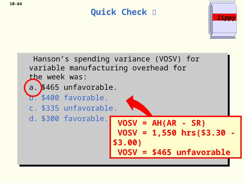
Hanson’s spending variance (VOSV) for variable manufacturing overhead forthe week was:a. $465 unfavorable.b. $400 favorable.c. $335 unfavorable.d. $300 favorable.

Hanson’s spending variance (VOSV) for variable manufacturing overhead forthe week was:a. $465 unfavorable.b. $400 favorable.c. $335 unfavorable.d. $300 favorable.

Quick Check

VOSV = AH(AR - SR) VOSV = 1,550 hrs($3.30 - $3.00) VOSV = $465 unfavorable

Zippy

10-65

Hanson’s efficiency variance (VOEV) for variable

manufacturing overhead for the week was:a. $435 unfavorable.b. $435 favorable.c. $150 unfavorable.d. $150 favorable.

Hanson’s efficiency variance (VOEV) for variable

manufacturing overhead for the week was:a. $435 unfavorable.b. $435 favorable.c. $150 unfavorable.d. $150 favorable.

Quick Check Zippy

10-66

Hanson’s efficiency variance (VOEV) for variable

manufacturing overhead for the week was:a. $435 unfavorable.b. $435 favorable.c. $150 unfavorable.d. $150 favorable.

Hanson’s efficiency variance (VOEV) for variable

manufacturing overhead for the week was:a. $435 unfavorable.b. $435 favorable.c. $150 unfavorable.d. $150 favorable.

Quick Check

VOEV = SR(AH - SH) VOEV = $3.00(1,550 hrs - 1,500 hrs) VOEV = $150 unfavorable

1,000 units × 1.5 hrs per unit

Zippy

10-67

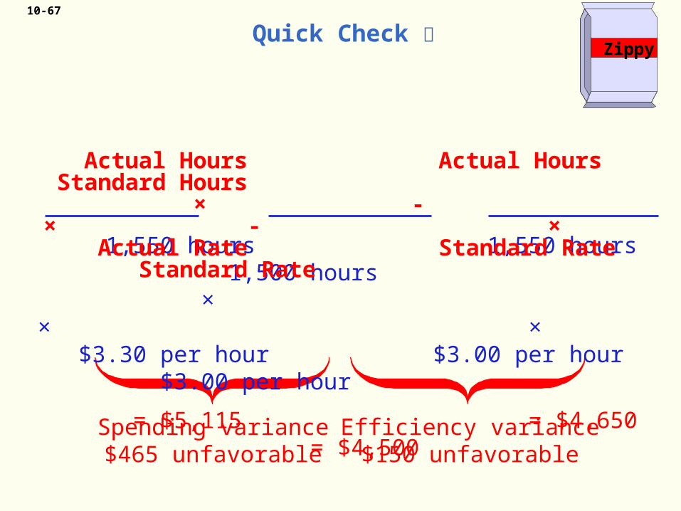
Spending variance$465 unfavorable

Efficiency variance$150 unfavorable

1,550 hours 1,550 hours 1,500 hours × × × $3.30 per hour $3.00 per hour $3.00 per hour

= $5,115 = $4,650 = $4,500

Actual Hours Actual Hours Standard Hours × - × - × Actual Rate Standard Rate Standard Rate

ZippyQuick Check

10-68Variance Analysis and

Management by Exception

How do I knowwhich variances to investigate?

Larger variances, in dollar amount

or as a percentage of the

standard, are investigated first.

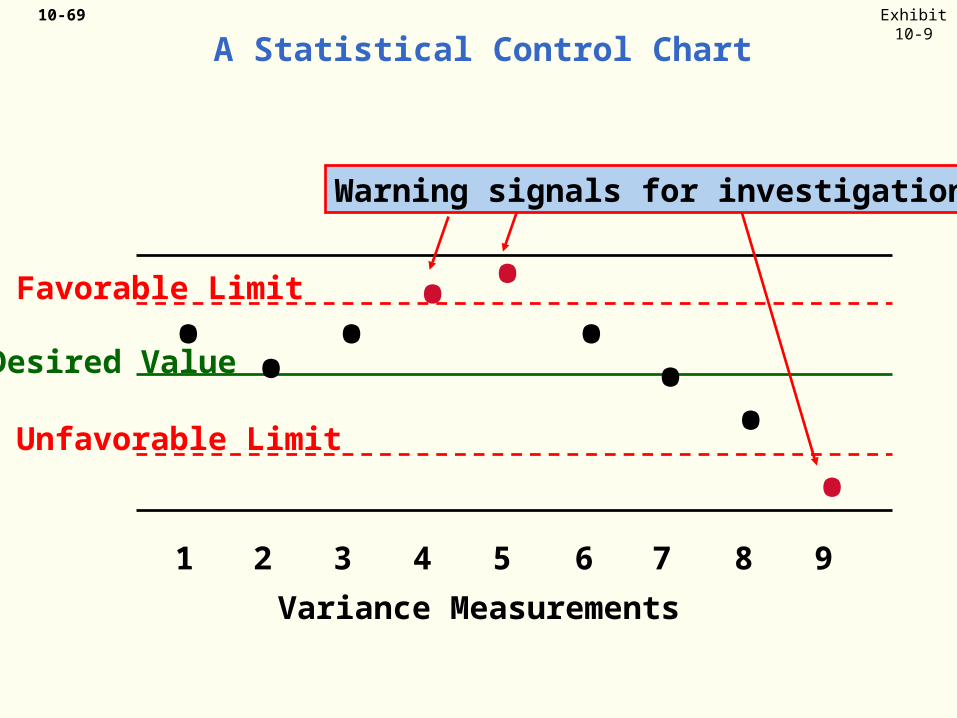
10-69

A Statistical Control Chart

1 2 3 4 5 6 7 8 9

Variance Measurements

Favorable Limit

Unfavorable Limit

• • •• •

••

••

Warning signals for investigation

Desired Value

Exhibit10-9

10-70

Learning Objective 6

Compute delivery cycle time, throughput time,

and manufacturingcycle efficiency (MCE).

10-71

Process time is the only value-added time.

Delivery Performance Measures

Wait TimeProcess Time + Inspection Time

+ Move Time + Queue Time

Delivery Cycle Time

Order Received

ProductionStarted

Goods Shipped

Throughput Time

10-72

Delivery Performance Measures

ManufacturingCycle

Efficiency

Value-added time

Manufacturing cycle time=

Wait TimeProcess Time + Inspection Time

+ Move Time + Queue Time

Delivery Cycle Time

Order Received

ProductionStarted

Goods Shipped

Throughput Time

10-73

Quick Check

A TQM team at Narton Corp has recorded the following average times for production:

Wait 3.0 days Move 0.5 days Inspection 0.4 days Queue 9.3 days Process 0.2 days

What is the throughput time? a. 10.4 daysb. 0.2 daysc. 4.1 daysd. 13.4 days

A TQM team at Narton Corp has recorded the following average times for production:

Wait 3.0 days Move 0.5 days Inspection 0.4 days Queue 9.3 days Process 0.2 days

What is the throughput time? a. 10.4 daysb. 0.2 daysc. 4.1 daysd. 13.4 days

10-74

A TQM team at Narton Corp has recorded the following average times for production:

Wait 3.0 days Move 0.5 days Inspection 0.4 days Queue 9.3 days Process 0.2 days

What is the throughput time? a. 10.4 daysb. 0.2 daysc. 4.1 daysd. 13.4 days

A TQM team at Narton Corp has recorded the following average times for production:

Wait 3.0 days Move 0.5 days Inspection 0.4 days Queue 9.3 days Process 0.2 days

What is the throughput time? a. 10.4 daysb. 0.2 daysc. 4.1 daysd. 13.4 days

Quick Check

Throughput time = Process + Inspection + Move + Queue = 0.2 days + 0.4 days + 0.5 days + 9.3 days = 10.4 days

10-75

Quick Check

A TQM team at Narton Corp has recorded the following average times for production:

Wait 3.0 days Move 0.5 days Inspection 0.4 days Queue 9.3 days Process 0.2 days

What is the Manufacturing Cycle Efficiency? a. 50.0%b. 1.9%c. 52.0%d. 5.1%

A TQM team at Narton Corp has recorded the following average times for production:

Wait 3.0 days Move 0.5 days Inspection 0.4 days Queue 9.3 days Process 0.2 days

What is the Manufacturing Cycle Efficiency? a. 50.0%b. 1.9%c. 52.0%d. 5.1%

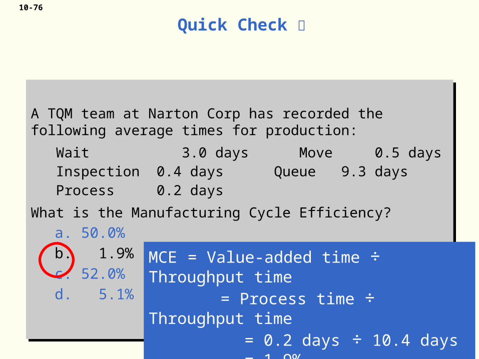
10-76

A TQM team at Narton Corp has recorded the following average times for production:

Wait 3.0 days Move 0.5 days Inspection 0.4 days Queue 9.3 days Process 0.2 days

What is the Manufacturing Cycle Efficiency?

a. 50.0%b. 1.9%c. 52.0%d. 5.1%

A TQM team at Narton Corp has recorded the following average times for production:

Wait 3.0 days Move 0.5 days Inspection 0.4 days Queue 9.3 days Process 0.2 days

What is the Manufacturing Cycle Efficiency?

a. 50.0%b. 1.9%c. 52.0%d. 5.1%

Quick Check

MCE = Value-added time ÷ Throughput time

= Process time ÷ Throughput time

= 0.2 days ÷ 10.4 days = 1.9%

10-77

Quick Check

A TQM team at Narton Corp has recorded the following average times for production:

Wait 3.0 days Move 0.5 days Inspection 0.4 days Queue 9.3 days Process 0.2 days

What is the delivery cycle time? a. 0.5 daysb. 0.7 daysc. 13.4 daysd. 10.4 days

A TQM team at Narton Corp has recorded the following average times for production:

Wait 3.0 days Move 0.5 days Inspection 0.4 days Queue 9.3 days Process 0.2 days

What is the delivery cycle time? a. 0.5 daysb. 0.7 daysc. 13.4 daysd. 10.4 days

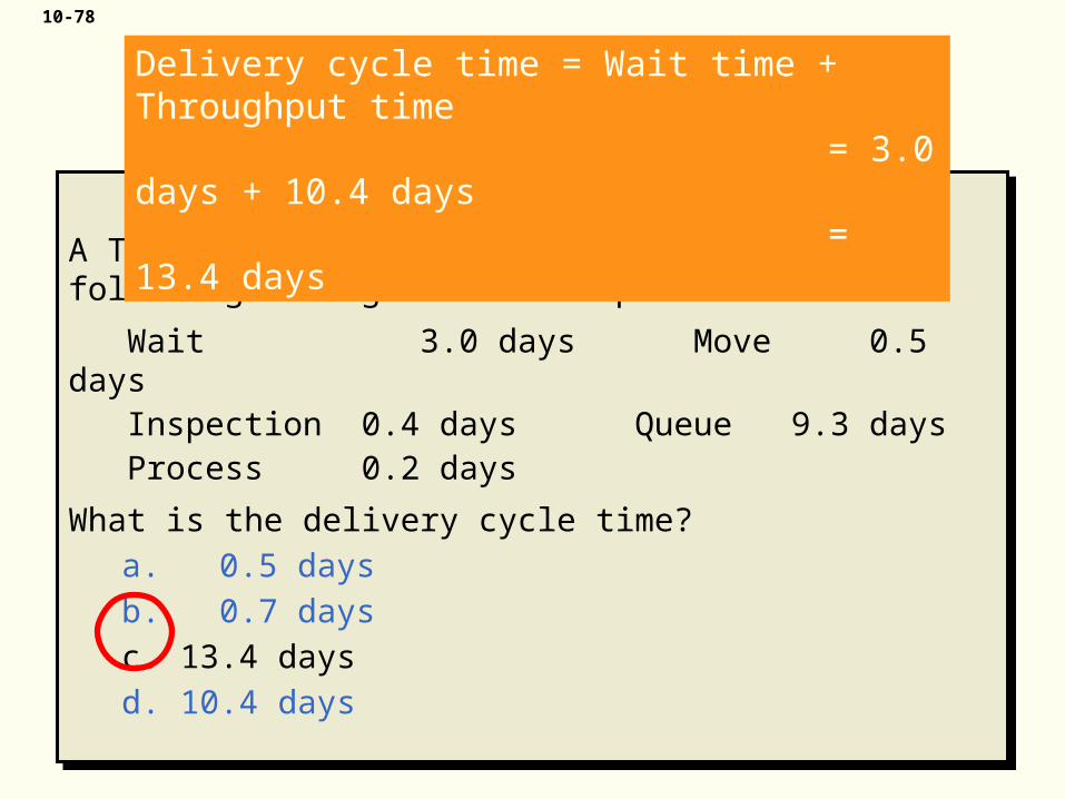
10-78

A TQM team at Narton Corp has recorded the following average times for production:

Wait 3.0 days Move 0.5 days Inspection 0.4 days Queue 9.3 days Process 0.2 days

What is the delivery cycle time? a. 0.5 daysb. 0.7 daysc. 13.4 daysd. 10.4 days

A TQM team at Narton Corp has recorded the following average times for production:

Wait 3.0 days Move 0.5 days Inspection 0.4 days Queue 9.3 days Process 0.2 days

What is the delivery cycle time? a. 0.5 daysb. 0.7 daysc. 13.4 daysd. 10.4 days

Quick Check Delivery cycle time = Wait time + Throughput time = 3.0 days + 10.4 days = 13.4 days

10-79

End of Chapter 10