chapter 11 an alternative view of risk and returnfinance-agruni.yolasite.com/resources/თავი...

An Alternative Viewof Risk and ReturnThe Arbitrage Pricing Theory

In January 2006, Yahoo!, Apple Computer, and Dutch semiconductor company ASML joined a host of other companies in announcing operating results. As you might expect, news such as this tends to move stock prices. Yahoo!, for example, reported a profit increase of 83 percent and a revenue increase of 39 percent. But investors didn’t say “Yahoo!” Instead, the stock price dropped by 12 percent when the market opened. Apple announced revenues for the most recent quarter of $5.75 billion, an increase of 65 percent over the same quarter in the previous year, and the company’s net income nearly doubled to $565 million. So, did investors cheer?

Not exactly: The stock price fell by 2 percent. Finally, ASML announced its earnings were less than half of the earnings from the same quarter in the previous year, on a sales decline of 30 percent. Even with this apparently troubling news, the company’s stock jumped over 6 percent. Two of these announcements seem positive, yet the stock price fell. The third announcement seems negative, yet the stock price jumped. So when is good news really good news? The answer is fundamental to understanding risk and return, and the good news is this chapter explores it in some detail.

C H A P T E R

11

320

11.1 Factor Models: Announcements, Surprises, and Expected ReturnsWe learned in the previous chapter how to construct portfolios and how to evaluate their returns. We now step back and examine the returns on individual securities more closely. By doing this we will find that the portfolios inherit and alter the properties of the securities they comprise. To be concrete, let us consider the return on the stock of a company called Flyers. What will determine this stock’s return in, say, the coming month? The return on any stock traded in a financial market consists of two parts. First, the nor-mal or expected return from the stock is the part of the return that shareholders in the market predict or expect. It depends on all of the information shareholders have that bears on the stock, and it uses all of our understanding of what will influence the stock in the next month. The second part is the uncertain or risky return on the stock. This is the portion that comes from information that will be revealed within the month. The list of such informa-tion is endless, but here are some examples:

• News about Flyers’ research.

• Government figures released for the gross national product (GNP).

ros05902_ch11.indd 320ros05902_ch11.indd 320 9/25/06 10:38:32 AM9/25/06 10:38:32 AM

Chapter 11 An Alternative View of Risk and Return 321

• Results of the latest arms control talks.

• Discovery that a rival’s product has been tampered with.

• News that Flyers’ sales figures are higher than expected.

• A sudden drop in interest rates.

• The unexpected retirement of Flyers’ founder and president.

A way to write the return on Flyers’ stock in the coming month, then, is:

R � R– � U

where R is the actual total return in the month, R– is the expected part of the return, and U

stands for the unexpected part of the return. We must exercise some care in studying the effect of these or other news items on the return. For example, the government might give us GNP or unemployment figures for this month, but how much of that is new information for shareholders? Surely, at the beginning of the month, shareholders will have some idea or forecast of what the monthly GNP will be. To the extent to which the shareholders had forecast the government’s announcement, that forecast should be factored into the expected part of the return as of the beginning of the month, R

–. On the other hand, insofar as the announcement by the government is a sur-

prise and to the extent to which it influences the return on the stock, it will be part of U, the unanticipated part of the return. As an example, suppose shareholders in the market had forecast that the GNP increase this month would be 0.5 percent. If GNP influences our company’s stock, this forecast will be part of the information shareholders use to form the expectation, R

–, of the monthly

return. If the actual announcement this month is exactly 0.5 percent, the same as the fore-cast, then the shareholders learned nothing new, and the announcement is not news. It is like hearing a rumor about a friend when you knew it all along. Another way of saying this is that shareholders had already discounted the announcement. This use of the word dis-count is different from that in computing present value, but the spirit is similar. When we discount a dollar in the future, we say that it is worth less to us because of the time value of money. When we discount an announcement or a news item in the future, we mean that it has less impact on the market because the market already knew much of it. On the other hand, suppose the government announced that the actual GNP increase during the year was 1.5 percent. Now shareholders have learned something—that the increase is one percentage point higher than they had forecast. This difference between the actual result and the forecast, one percentage point in this example, is sometimes called the innovation or surprise. Any announcement can be broken into two parts, the anticipated or expected part and the surprise or innovation:

Announcement � Expected part � Surprise

The expected part of any announcement is part of the information the market uses to form the expectation, R

–, of the return on the stock. The surprise is the news that influences the

unanticipated return on the stock, U. For example, to open the chapter, we compared Yahoo!, Apple Computer, and ASML. In Yahoo!’s case, even though the company’s revenue and profits jumped substantially, neither number met investor expectations. In Apple’s case, in addition to the good earn-ings, the company announced that sales in the next quarter would be lower than previously expected. And for ASML, even though sales and profits were below the previous year, both numbers exceeded expectations.


322 Part III Risk

To give another example, if shareholders of a company knew in January that the presi-dent of a firm was going to resign, the official announcement in February will be fully expected and will be discounted by the market. Because the announcement was expected before February, its influence on the stock will have taken place before February. The announcement itself in February will contain no surprise, and the stock’s price should not change at all at the announcement in February. When we speak of news, then, we refer to the surprise part of any announcement and not the portion that the market has expected and therefore has already discounted.

11.2 Risk: Systematic and UnsystematicThe unanticipated part of the return—that portion resulting from surprises—is the true risk of any investment. After all, if we got what we had expected, there would be no risk and no uncertainty. There are important differences, though, among various sources of risk. Look at our previous list of news stories. Some of these stories are directed specifically at Flyers, and some are more general. Which of the news items are of specific importance to Flyers? Announcements about interest rates or GNP are clearly important for nearly all com-panies, whereas the news about Flyers’ president, its research, its sales, or the affairs of a rival company are of specific interest to Flyers. We will divide these two types of announce-ments and the resulting risk, then, into two components: a systematic portion, called sys-tematic risk, and the remainder, which we call specific or unsystematic risk. The following definitions describe the difference:

• A systematic risk is any risk that affects a large number of assets, each to a greater or lesser degree.

• An unsystematic risk is a risk that specifically affects a single asset or a small group of assets.1

Uncertainty about general economic conditions, such as GNP, interest rates, or inflation, is an example of systematic risk. These conditions affect nearly all stocks to some degree. An unanticipated or surprise increase in inflation affects wages and the costs of the supplies that companies buy, the value of the assets that companies own, and the prices at which companies sell their products. These forces to which all companies are susceptible are the essence of systematic risk. In contrast, the announcement of a small oil strike by a company may affect that com-pany alone or a few other companies. Certainly, it is unlikely to have an effect on the world oil market. To stress that such information is unsystematic and affects only some specific companies, we sometimes call it an idiosyncratic risk. The distinction between a systematic risk and an unsystematic risk is never as exact as we make it out to be. Even the most narrow and peculiar bit of news about a company ripples through the economy. It reminds us of the tale of the war that was lost because one horse lost a shoe; even a minor event may have an impact on the world. But this degree of hairsplitting should not trouble us much. To paraphrase a Supreme Court justice’s com-ment when speaking of pornography, we may not be able to define a systematic risk and an unsystematic risk exactly, but we know them when we see them.

1In the previous chapter, we briefly mentioned that unsystematic risk is risk that can be diversified away in a large portfolio. This result will also follow from the present analysis.



This permits us to break down the risk of Flyers’ stock into its two components: the systematic and the unsystematic. As is traditional, we will use the Greek epsilon, �, to rep-resent the unsystematic risk and write:

R � R– � U

� R– � m � �

where we have used the letter m to stand for the systematic risk. Sometimes systematic risk is referred to as market risk. This emphasizes the fact that m influences all assets in the market to some extent. The important point about the way we have broken the total risk, U, into its two com-ponents, m and �, is that �, because it is specific to the company, is unrelated to the specific risk of most other companies. For example, the unsystematic risk on Flyers’ stock, �F, is unrelated to the unsystematic risk of Xerox’s stock, �X. The risk that Flyers’ stock will go up or down because of a discovery by its research team—or its failure to discover some-thing—probably is unrelated to any of the specific uncertainties that affect Xerox stock. Using the terms of the previous chapter, this means that the unsystematic risks of Flyers’ stock and Xerox’s stock are unrelated to each other, or uncorrelated. In the symbols of statistics:

Corr(�F, �X) � 0

11.3 Systematic Risk and BetasThe fact that the unsystematic parts of the returns on two companies are unrelated to each other does not mean that the systematic portions are unrelated. On the contrary, because both companies are influenced by the same systematic risks, individual companies’ sys-tematic risks and therefore their total returns will be related. For example, a surprise about inflation will influence almost all companies to some extent. How sensitive is Flyers’ stock return to unanticipated changes in inflation? If Flyers’ stock tends to go up on news that inflation is exceeding expectations, we would say that it is positively related to inflation. If the stock goes down when inflation exceeds expectations and up when inflation falls short of expectations, it is negatively related. In the unusual case where a stock’s return is uncorrelated with inflation surprises, inflation has no effect on it. We capture the influence of a systematic risk like inflation on a stock by using the beta coefficient. The beta coefficient, �, tells us the response of the stock’s return to a systematic risk. In the previous chapter, beta measured the responsiveness of a security’s return to a specific risk factor, the return on the market portfolio. We used this type of responsiveness to develop the capital asset pricing model. Because we now consider many types of system-atic risks, our current work can be viewed as a generalization of our work in the previous chapter. If a company’s stock is positively related to the risk of inflation, that stock has a posi-tive inflation beta. If it is negatively related to inflation, its inflation beta is negative; and if it is uncorrelated with inflation, its inflation beta is zero. It’s not hard to imagine some stocks with positive inflation betas and other stocks with negative inflation betas. The stock of a company owning gold mines will probably have a positive inflation beta because an unanticipated rise in inflation is usually associated with an increase in gold prices. On the other hand, an automobile company facing stiff foreign competition might find that an increase in inflation means that the wages it pays are higher, but that it cannot raise its prices to cover the increase. This profit squeeze, as the company’s expenses rise faster than its revenues, would give its stock a negative inflation beta.


324 Part III Risk

Some companies that have few assets and that act as brokers—buying items in com-petitive markets and reselling them in other markets—might be relatively unaffected by inflation because their costs and their revenues would rise and fall together. Their stock would have an inflation beta of zero. Some structure is useful at this point. Suppose we have identified three systematic risks on which we want to focus. We may believe that these three are sufficient to describe the systematic risks that influence stock returns. Three likely candidates are inflation, GNP, and interest rates. Thus, every stock will have a beta associated with each of these system-atic risks: an inflation beta, a GNP beta, and an interest rate beta. We can write the return on the stock, then, in the following form:

R � R– � U

� R– � m � �

� R– � �IFI � �GNPFGNP � �rFr � �

where we have used the symbol �I to denote the stock’s inflation beta, �GNP for its GNP beta, and �r to stand for its interest rate beta. In the equation, F stands for a surprise, whether it be in inflation, GNP, or interest rates. Let us go through an example to see how the surprises and the expected return add up to produce the total return, R, on a given stock. To make it more familiar, suppose that the return is over a horizon of a year and not just a month. Suppose that at the beginning of the year, inflation is forecast to be 5 percent for the year, GNP is forecast to increase by 2 percent and interest rates are expected not to change. Suppose the stock we are looking at has the following betas:

�I � 2

�GNP � 1

�r � �1.8

The magnitude of the beta describes how great an impact a systematic risk has on a stock’s returns. A beta of �1 indicates that the stock’s return rises and falls one for one with the systematic factor. This means, in our example, that because the stock has a GNP beta of 1, it experiences a 1 percent increase in return for every 1 percent surprise increase in GNP. If its GNP beta were �2, it would fall by 2 percent when there was an unanticipated increase of 1 percent in GNP, and it would rise by 2 percent if GNP experienced a surprise 1 percent decline. Let us suppose that during the year the following events occur: Inflation rises by 7 percent, GNP rises by only 1 percent, and interest rates fall by 2 percent. Suppose we learn some good news about the company, perhaps that it is succeeding quickly with some new business strategy, and that this unanticipated development contributes 5 percent to its return. In other words:

� � 5%

Let us assemble all of this information to find what return the stock had during the year. First we must determine what news or surprises took place in the systematic factors. From our information we know that:

Expected infl ation � 5%

Expected GNP change � 2%

and:

Expected change in interest rates � 0%



This means that the market had discounted these changes, and the surprises will be the dif-ference between what actually takes place and these expectations:

FI � Surprise in infl ation

� Actual infl ation � Expected infl ation

� 7% � 5%

� 2%

Similarly:

FGNP � Surprise in GNP

� Actual GNP � Expected GNP

� 1% � 2%

� �1%

and:

Fr � Surprise in change in interest rates

� Actual change � Expected change

� �2% � 0%

� �2%

The total effect of the systematic risks on the stock return, then, is:

m � Systematic risk portion of return

� �IFI � �GNPFGNP � �rFr

� [2 � 2%] � [1 � (�1%)] � [(�1.8) � (�2%)]

� 6.6%

Combining this with the unsystematic risk portion, the total risky portion of the return on the stock is:

m � � � 6.6% � 5% � 11.6%

Last, if the expected return on the stock for the year was, say, 4 percent, the total return from all three components will be:

R � R– � m � �

� 4% � 6.6% � 5%

� 15.6%

The model we have been looking at is called a factor model, and the systematic sources of risk, designated F, are called the factors. To be perfectly formal, a k-factor model is a model where each stock’s return is generated by:

R � R– � �1F1 � �2F2 � . . . � �kFk � �

where � is specific to a particular stock and uncorrelated with the � term for other stocks. In our preceding example we had a three-factor model. We used inflation, GNP, and the change in interest rates as examples of systematic sources of risk, or factors. Researchers have not settled on what is the correct set of factors. Like so many other questions, this might be one of those matters that is never laid to rest. In practice, researchers frequently use a one-factor model for returns. They do not use all of the sorts of economic factors we used previously as examples; instead they use an


326 Part III Risk

index of stock market returns—like the S&P 500, or even a more broadly based index with more stocks in it—as the single factor. Using the single-factor model we can write returns like this:

R � R– � �(RS&P500 � R

–S&P500) � �

Where there is only one factor (the returns on the S&P 500 portfolio index), we do not need to put a subscript on the beta. In this form (with minor modifications) the factor model is called a market model. This term is employed because the index that is used for the factor is an index of returns on the whole (stock) market. The market model is written as:

R � R– � �(RM � R

–M) � �

where RM is the return on the market portfolio.2 The single � is called the beta coefficient.

11.4 Portfolios and Factor ModelsNow let us see what happens to portfolios of stocks when each of the stocks follows a one-factor model. For purposes of discussion, we will take the coming one-month period and examine returns. We could have used a day or a year or any other period. If the period represents the time between decisions, however, we would rather it be short than long, and a month is a reasonable time frame to use. We will create portfolios from a list of N stocks, and we will use a one-factor model to capture the systematic risk. The ith stock in the list will therefore have returns:

Ri � R–

i � �iF � �i (11.1)

where we have subscripted the variables to indicate that they relate to the ith stock. Notice that the factor F is not subscripted. The factor that represents systematic risk could be a surprise in GNP, or we could use the market model and let the difference between the S&P 500 return and what we expect that return to be, RS&P500 � R

–S&P500, be the factor. In either

case, the factor applies to all of the stocks. The �i is subscripted because it represents the unique way the factor influences the ith stock. To recapitulate our discussion of factor models, if �i is zero, the returns on the ith stock are:

Ri � R–

i � �i

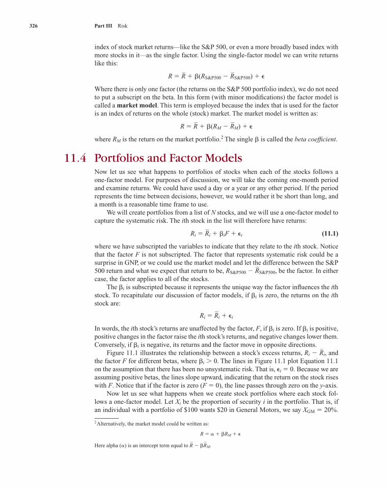
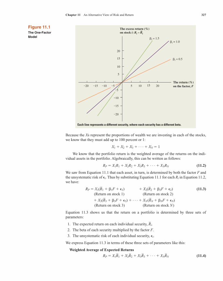
In words, the ith stock’s returns are unaffected by the factor, F, if �i is zero. If �i is positive, positive changes in the factor raise the ith stock’s returns, and negative changes lower them. Conversely, if �i is negative, its returns and the factor move in opposite directions. Figure 11.1 illustrates the relationship between a stock’s excess returns, Ri � R

–i, and

the factor F for different betas, where �i � 0. The lines in Figure 11.1 plot Equation 11.1 on the assumption that there has been no unsystematic risk. That is, �i � 0. Because we are assuming positive betas, the lines slope upward, indicating that the return on the stock rises with F. Notice that if the factor is zero (F � 0), the line passes through zero on the y-axis. Now let us see what happens when we create stock portfolios where each stock fol-lows a one-factor model. Let Xi be the proportion of security i in the portfolio. That is, if an individual with a portfolio of $100 wants $20 in General Motors, we say XGM � 20%.

2Alternatively, the market model could be written as:

R � � � �RM � �

Here alpha (�) is an intercept term equal to R– � �R

–M.



Because the Xs represent the proportions of wealth we are investing in each of the stocks, we know that they must add up to 100 percent or 1:

X1 � X2 � X3 � . . . � XN � 1

We know that the portfolio return is the weighted average of the returns on the indi-vidual assets in the portfolio. Algebraically, this can be written as follows:

RP � X1R1 � X2R2 � X3R3 � . . . � XNRN (11.2)

We saw from Equation 11.1 that each asset, in turn, is determined by both the factor F and the unsystematic risk of �i. Thus by substituting Equation 11.1 for each Ri in Equation 11.2, we have:

RP � X1(R–

1 � �1F � �1) � X2(R–

2 � �2F � �2) (11.3) (Return on stock 1) (Return on stock 2)

� X3(R–

3 � �3F � �3) � . . . � XN (R–

N � �NF � �N) (Return on stock 3) (Return on stock N )

Equation 11.3 shows us that the return on a portfolio is determined by three sets of parameters:

1. The expected return on each individual security, R–

i.

2. The beta of each security multiplied by the factor F.

3. The unsystematic risk of each individual security, �i.

We express Equation 11.3 in terms of these three sets of parameters like this:

Weighted Average of Expected Returns

RP � X1R–

1 � X2R–

2 � X3R–

3 � . . . � XNR–

N (11.4)

The excess return (%)on stock i: Ri – Ri

The return (%)on the factor, F

–5

15

10

5

–10

–15

20

–20 –15 –10 –5 5 10 15 20

�i = 1.5�i = 1.0

�i = 0.5

–20

Figure 11.1The One-Factor Model

Each line represents a different security, where each security has a different beta.


328 Part III Risk

Weighted Average of Betas � F

� (X1�1 � X2�2 � X3�3 � . . . � XN�N)F

Weighted Average of Unsystematic Risks

� X1�1 � X2�2 � X3�3 � . . . � XN�N

This rather imposing equation is actually straightforward. The first row is the weighted average of each security’s expected return. The items in the parentheses of the second row represent the weighted average of each security’s beta. This weighted average is, in turn, multiplied by the factor F. The third row represents a weighted average of the unsystematic risks of the individual securities. Where does uncertainty appear in Equation 11.4? There is no uncertainty in the first row because only the expected value of each security’s return appears there. Uncertainty in the second row is reflected by only one item, F. That is, while we know that the expected value of F is zero, we do not know what its value will be over a particular period. Uncer-tainty in the third row is reflected by each unsystematic risk, �i.

Portfolios and Diversifi cationIn the previous sections of this chapter, we expressed the return on a single security in terms of our factor model. Portfolios were treated next. Because investors generally hold diversified portfolios, we now want to know what Equation 11.4 looks like in a large or diversified portfolio.3

As it turns out, something unusual occurs to Equation 11.4: The third row actually disap pears in a large portfolio. To see this, consider a gambler who divides $1,000 by bet-ting on red over many spins of the roulette wheel. For example, he may participate in 1,000 spins, betting $1 at a time. Though we do not know ahead of time whether a particular spin will yield red or black, we can be confident that red will win about 50 percent of the time. Ignoring the house take, the investor can be expected to end up with just about his original $1,000. Though we are concerned with stocks, not roulette wheels, the same principle applies. Each security has its own unsystematic risk, where the surprise for one stock is unrelated to the surprise of another stock. By investing a small amount in each security, we bring the weighted average of the unsystematic risks close to zero in a large portfolio.4

Although the third row completely vanishes in a large portfolio, nothing unusual occurs in either row 1 or row 2. Row 1 remains a weighted average of the expected returns on the individual securities as securities are added to the portfolio. Because there is no uncer-tainty at all in the first row, there is no way for diversification to cause this row to vanish. The terms inside the parentheses of the second row remain a weighted average of the betas. They do not vanish, either, when securities are added. Because the factor F is unaffected when securities are added to the portfolios, the second row does not vanish. Why does the third row vanish while the second row does not, though both rows reflect uncertainty? The key is that there are many unsystematic risks in row 3. Because these risks are independent of each other, the effect of diversification becomes stronger as we add more assets to the portfolio. The resulting portfolio becomes less and less risky, and the

3Technically, we can think of a large portfolio as one where an investor keeps increasing the number of securi-ties without limit. In practice, effective diversification would occur if at least a few dozen securities were held.4More precisely, we say that the weighted average of the unsystematic risk approaches zero as the number of equally weighted securities in a portfolio approaches infinity.



Diversification and Unsystematic Risk The preceding material can be further explained by the following example. We keep our one-factor model here but make three specific assumptions:

1. All securities have the same expected return of 10 percent. This assumption implies that the first row of Equation 11.4 must also equal 10 percent because this row is a weighted average of the expected returns of the individual securities.

2. All securities have a beta of 1. The sum of the terms inside the parentheses in the second row of Equation 11.4 must equal 1 because these terms are a weighted average of the individual betas. Because the terms inside the parentheses are multiplied by F, the value of the second row is 1 � F � F.

3. In this example, we focus on the behavior of one individual, Walter V. Bagehot. Mr. Bagehot decides to hold an equally weighted portfolio. That is, the proportion of each security in his portfolio is 1/N.

We can express the return on Mr. Bagehot’s portfolio as follows:

Return on Walter V. Bagehot’s Portfolio

R F

N N N NP N= + + ∈ + ∈ + ∈ + + ∈

⎛

⎝⎜⎜⎜⎜

⎞

⎠⎟⎟⎟10

1 1 1 11 2 3% . . .

⎟⎟⎟ (11.4�)

From From From row 3 of row 1 of row 2 of Equation 11.4 Equation 11.4 Equation11.4

We mentioned before that as N increases without limit, row 3 of Equation 11.4 becomes equal to zero.5 Thus, the return to Walter Bagehot’s portfolio when the number of securities is very large is

RP � 10% � F (11.4�)

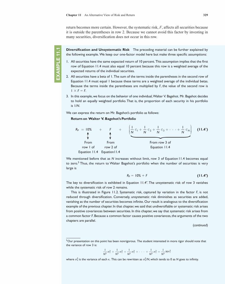
The key to diversification is exhibited in Equation 11.4. The unsystematic risk of row 3 vanishes while the systematic risk of row 2 remains. This is illustrated in Figure 11.2. Systematic risk, captured by variation in the factor F, is not reduced through diversification. Conversely, unsystematic risk diminishes as securities are added, vanishing as the number of securities becomes infinite. Our result is analogous to the diversification example of the previous chapter. In that chapter, we said that undiversifiable or systematic risk arises from positive covariances between securities. In this chapter, we say that systematic risk arises from a common factor F. Because a common factor causes positive covariances, the arguments of the two chapters are parallel.

EX

AM

PL

E 1

1.1

5Our presentation on this point has been nonrigorous. The student interested in more rigor should note that the variance of row 3 is:

1 1 1 1 12

22

22

22

22

2

N N N N NN ∈ ∈ ∈ ∈ ∈+ + + + =. . .

where 2� is the variance of each �. This can be rewritten as 2

�/N, which tends to 0 as N goes to infinity.

�

(continued)

return becomes more certain. However, the systematic risk, F, affects all securities because it is outside the parentheses in row 2. Because we cannot avoid this factor by investing in many securities, diversification does not occur in this row.


330 Part III Risk

2P

Systematicrisk

N, number ofsecuritiesin portfolio

Unsystematicrisk

Total risk, �

Figure 11.2 Diversification and the Portfolio Risk for an Equally Weighted Portfolio

Total risk decreases as the number of securities in the portfolio rises. This

drop occurs only in the unsystematic risk component. Systematic risk is

unaffected by diversifi cation.

11.5 Betas and Expected Returns

The Linear RelationshipWe have argued many times that the expected return on a security compensates for its risk. In the previous chapter we showed that market beta (the standardized covariance of the security’s returns with those of the market) was the appropriate measure of risk under the assumptions of homogeneous expectations and riskless borrowing and lending. The capital asset pricing model, which posited these assumptions, implied that the expected return on a security was positively (and linearly) related to its beta. We will find a similar relationship between risk and return in the one-factor model of this chapter. We begin by noting that the relevant risk in large and well-diversified portfolios is all systematic because unsystematic risk is diversified away. An implication is that when a well-diversified shareholder considers changing her holdings of a particular stock, she can ignore the security’s unsystematic risk. Notice that we are not claiming that stocks, like portfolios, have no unsystematic risk. Nor are we saying that the unsystematic risk of a stock will not affect its returns. Stocks do have unsystematic risk, and their actual returns do depend on the unsystematic risk. Because this risk washes out in a well-diversified portfolio, however, shareholders can ignore this unsystematic risk when they consider whether to add a stock to their portfolio. Therefore, if shareholders are ignoring the unsystematic risk, only the systematic risk of a stock can be related to its expected return. This relationship is illustrated in the security market line of Figure 11.3. Points P, C, A, and L all lie on the line emanating from the risk-free rate of 10 percent. The points representing each of these four assets can be created by combinations of the risk-free rate and any of the other three assets. For example, because A has a beta of 2.0 and P has a beta of 1.0, a portfolio of 50 percent in asset A and 50 percent in the riskless rate has the same beta as asset P. The risk-free rate is 10 percent and the expected return on security A is 35 percent, implying that the combination’s return of 22.5 percent [(10% � 35%)/2] is identical to security P’s expected return. Because security P has both the same beta and the same expected return as a combination of the riskless asset and security A, an individual is



Beta: �i1 2

35

22.5

RF =10

Expected returns (%)Ri

L

A

C

B

P

Security market line

Figure 11.3A Graph of Beta and Expected Return for Individual Stocks under the One-Factor Model

equally inclined to add a small amount of security P and to add a small amount of this com-bination to her portfolio. However, the unsystematic risk of security P need not be equal to the unsystematic risk of the combination of security A and the risk-free rate because unsystematic risk is diversified away in a large portfolio. Of course, the potential combinations of points on the security market line are endless. We can duplicate P by combinations of the risk-free rate and either C or L (or both of them). We can duplicate C (or A or L) by borrowing at the risk-free rate to invest in P. The infinite number of points on the security market line that are not labeled can be used as well. Now consider security B. Because its expected return is below the line, no investor would hold it. Instead, the investor would prefer security P, a combination of security A and the riskless asset, or some other combination. Thus, security B’s price is too high. Its price will fall in a competitive market, forcing its expected return back up to the line in equilibrium. The preceding discussion allows us to provide an equation for the security market line of Figure 11.3. We know that a line can be described algebraically from two points. It is perhaps easiest to focus on the risk-free rate and asset P because the risk-free rate has a beta of 0 and P has a beta of 1. Because we know that the return on any zero-beta asset is RF and the expected return on asset P is R

–P, it can easily be shown that:

R– � RF � �(R

–P � RF) (11.5)

In Equation 11.5, R– can be thought of as the expected return on any security or portfolio

lying on the security market line. � is the beta of that security or portfolio.

The Market Portfolio and the Single FactorIn the CAPM the beta of a security measures the security’s responsiveness to movements in the market portfolio. In the one-factor model of the arbitrage pricing theory (APT) the beta of a security measures its responsiveness to the factor. We now relate the market portfolio to the single factor. A large, diversified portfolio has no unsystematic risk because the unsystematic risks of the individual securities are diversified away. Assuming enough securities so that the market portfolio is fully diversified and assuming that no security has a disproportionate market share, this portfolio is fully diversified and contains no unsystematic risk.6 In other

6This assumption is plausible in the real world. For example, even the market value of General Electric is only 3 percent to 4 percent of the market value of the S&P 500 Index.


332 Part III Risk

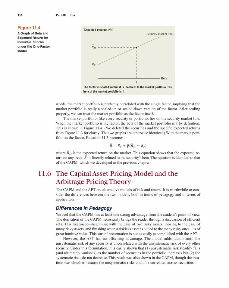
words, the market portfolio is perfectly correlated with the single factor, implying that the market portfolio is really a scaled-up or scaled-down version of the factor. After scaling properly, we can treat the market portfolio as the factor itself. The market portfolio, like every security or portfolio, lies on the security market line. When the market portfolio is the factor, the beta of the market portfolio is 1 by definition. This is shown in Figure 11.4. (We deleted the securities and the specific expected returns from Figure 11.3 for clarity: The two graphs are otherwise identical.) With the market port-folio as the factor, Equation 11.5 becomes:

R– � RF � �(R

–M � RF)

where R–

M is the expected return on the market. This equation shows that the expected re-turn on any asset, R

–, is linearly related to the security’s beta. The equation is identical to that

of the CAPM, which we developed in the previous chapter.

11.6 The Capital Asset Pricing Model and the Arbitrage Pricing TheoryThe CAPM and the APT are alternative models of risk and return. It is worthwhile to con-sider the differences between the two models, both in terms of pedagogy and in terms of application.

Differences in PedagogyWe feel that the CAPM has at least one strong advantage from the student’s point of view. The derivation of the CAPM necessarily brings the reader through a discussion of efficient sets. This treatment—beginning with the case of two risky assets, moving to the case of many risky assets, and finishing when a riskless asset is added to the many risky ones—is of great intuitive value. This sort of presentation is not as easily accomplished with the APT. However, the APT has an offsetting advantage. The model adds factors until the unsystematic risk of any security is uncorrelated with the unsystematic risk of every other security. Under this formulation, it is easily shown that (1) unsystematic risk steadily falls (and ultimately vanishes) as the number of securities in the portfolio increases but (2) the systematic risks do not decrease. This result was also shown in the CAPM, though the intu-ition was cloudier because the unsystematic risks could be correlated across securities.

Figure 11.4A Graph of Beta and Expected Return for Individual Stocks under the One-Factor Model

Expected returns (%)

Beta

Security market line

RM

RF

1

The factor is scaled so that it is identical to the market portfolio. The beta of the market portfolio is 1.



Differences in ApplicationOne advantage of the APT is that it can handle multiple factors while the CAPM ignores them. Although the bulk of our presentation in this chapter focused on the one-factor model, a multifactor model is probably more reflective of reality. That is, we must abstract from many marketwide and industrywide factors before the unsystematic risk of one security be-comes uncorrelated with the unsystematic risks of other securities. Under this multifactor version of the APT, the relationship between risk and return can be expressed as:

R– � RF � (R

–1 � RF)�1 � (R

–2 � RF)�2 � (R

–3 � RF)�3 � . . . � (R

–K � RF)�K (11.6)

In this equation, �1 stands for the security’s beta with respect to the first factor, �2 stands for the security’s beta with respect to the second factor, and so on. For example, if the first factor is GNP, �1 is the security’s GNP beta. The term R

–1 is the expected return on a security (or

portfolio) whose beta with respect to the first factor is 1 and whose beta with respect to all other factors is zero. Because the market compensates for risk, (R

–1 � RF) will be positive

in the normal case.7 (An analogous interpretation can be given to R–

2, R–

3, and so on.) The equation states that the security’s expected return is related to the security’s factor betas. The intuition in Equation 11.6 is straightforward. Each factor represents risk that cannot be diversified away. The higher a security’s beta with regard to a particular factor is, the higher is the risk that the security bears. In a rational world, the expected return on the security should compensate for this risk. Equation 11.6 states that the expected return is a summation of the risk-free rate plus the compensation for each type of risk that the security bears. As an example, consider a study where the factors were monthly growth in industrial production (IP), change in expected inflation (�EI), unanticipated inflation (UI), unantici-pated change in the risk premium between risky bonds and default-free bonds (URP), and unanticipated change in the difference between the return on long-term government bonds and the return on short-term government bonds (UBR).8 Using the period 1958–1984, the empirical results of the study indicated that the expected monthly return on any stock, R

–S,

can be described as:

R–

S � 0.0041 � 0.0136�IP � 0.0001��EI � 0.0006�UI � 0.0072�URP � 0.0052�UBR

Suppose a particular stock had the following betas: �IP � 1.1, ��EI � 2, �UI � 3,�URP � 0.1, �UBR � 1.6. The expected monthly return on that security would be:

R–

S � 0.0041 � 0.0136 � 1.1 � 0.0001 � 2 � 0.0006 � 3 � 0.0072 � 0.1 � 0.0052 � 1.6

� 0.0095

Assuming that a firm is unlevered and that one of the firm’s projects has risk equivalent to that of the firm, this value of 0.0095 (i.e., .95%) can be used as the monthly discount rate for the project. (Because annual data are often supplied for capital budgeting purposes, the annual rate of 0.120 [� (1.0095)12 � 1] might be used instead.) Because many factors appear on the right side of Equation 11.6, the APT formulation has the potential to measure expected returns more accurately than does the CAPM. How-ever, as we mentioned earlier, we cannot easily determine which are the appropriate factors. The factors in the preceding study were included for reasons of both common sense and convenience. They were not derived from theory.

7Actually, (R–

i � RF) could be negative in the case where factor i is perceived as a hedge of some sort.8N. Chen, R. Roll, and S. Ross, “Economic Forces and the Stock Market,” Journal of Business (July 1986).


334 Part III Risk

By contrast, the use of the market index in the CAPM formulation is implied by the theory of the previous chapter. We suggested in earlier chapters that the S&P 500 index mirrors stock market movements quite well. Using the Ibbotson-Sinquefield results show-ing that the yearly return on the S&P 500 index was, on average, 8.5 percent greater than the risk-free rate, the last chapter easily calculated expected returns on different securities from the CAPM.9

11.7 Empirical Approaches to Asset Pricing

Empirical ModelsThe CAPM and the APT by no means exhaust the models and techniques used in practice to measure the expected return on risky assets. Both the CAPM and the APT are risk-based models. They each measure the risk of a security by its beta(s) on some systematic factor(s), and they each argue that the expected excess return must be proportional to the beta(s). Although we have seen that this is intuitively appealing and has a strong basis in theory, there are alternative approaches. Most of these alternatives can be lumped under the broad heading of parametric or empirical models. The word empirical refers to the fact that these approaches are based less on some theory of how financial markets work and more on simply looking for regularities and relations in the history of market data. In these approaches the researcher specifies some parameters or attributes associated with the securities in question and then examines the data directly for a relation between these attributes and expected returns. For example, an extensive amount of research has been done on whether the expected return on a firm is related to its size. Is it true that small firms have higher average returns than large firms? Researchers have also examined a variety of accounting measures such as the ratio of the price of a stock to its accounting earnings, its P/E ratio, and the closely related ratio of the market value of the stock to the book value of the company, the M/B ratio. Here it might be argued that companies with low P/E’s or low M/B’s are “undervalued” and can be expected to have higher returns in the future. To use the empirical approach to determine the expected return, we would estimate the following equation:

R–

i � RF � kP/E (P/E)i � kM/B (M/B)i � ksize (size)P

where R–

i is the expected return of firm i, and where the k’s are coefficients that we estimate from stock market data. Notice that this is the same form as Equation 11.6 with the firm’s attributes in place of betas and with the k’s in place of the excess factor portfolio returns. When tested with data, these parametric approaches seem to do quite well. In fact, when comparisons are made between using parameters and using betas to predict stock returns, the parameters, such as P/E and M/B, seem to work better. There are a variety of possible explanations for these results, and the issues have certainly not been settled. Crit-ics of the empirical approach are skeptical of what they call data mining. The particular parameters that researchers work with are often chosen because they have been shown to be related to returns. For instance, suppose that you were asked to explain the change in SAT test scores over the past 40 years in some particular state. Suppose that to do this you searched through all of the data series you could find. After much searching, you might discover, for example, that the change in the scores was directly related to the jackrabbit

9Though many researchers assume that surrogates for the market portfolio are easily found, Richard Roll, “A Critique of the Asset Pricing Theory’s Tests,” Journal of Financial Economics (March 1977), argues that theabsence of a universally acceptable proxy for the market portfolio seriously impairs application of the theory. After all, the market must include real estate, racehorses, and other assets that are not in the stock market.



population in Arizona. We know that any such relation is purely accidental; but if you search long enough and have enough choices, you will find something even if it is not really there. It’s a bit like staring at clouds. After a while you will see clouds that look like any-thing you want—clowns, bears, or whatever—but all you are really doing is data mining. Needless to say, the researchers on these matters defend their work by arguing that they have not mined the data and have been very careful to avoid such traps by not snooping at the data to see what will work. Of course, as a matter of pure theory, because anyone in the market can easily look up the P/E ratio of a firm, we would certainly not expect to find that firms with low P/E’s did bet-ter than firms with high P/E’s simply because they were undervalued. In an efficient market, such public measures of undervaluation would be quickly exploited and would not last. Perhaps a better explanation for the success of empirical approaches lies in a syn-thesis of the risk-based approaches and the empirical methods. In an efficient market risk and return are related; so perhaps the parameters or attributes that appear to be related to returns are also better measures of risk. For example, if we were to find that low P/E firms outperformed high P/E firms and that this was true even for firms that had the same beta(s), then we would have at least two possible explanations. First, we could simply discard the risk-based theories as incorrect. Furthermore, we could argue that markets are inefficient and that buying low P/E stocks provides us with an opportunity to make higher than pre-dicted returns. Second, we could argue that both views of the world are correct and that the P/E is really just a better way to measure systematic risk—that is, beta(s)—than directly estimating beta from the data.

Style PortfoliosIn addition to their use as a platform for estimating expected returns, stock attributes are also widely used as a way of characterizing money management styles. For example, a portfolio that has a P/E ratio much in excess of the market average might be characterized as a high P/E or a growth stock portfolio. Similarly, a portfolio made up of stocks with an average P/E less than that for a market index might be characterized as a low P/E or a value portfolio. To evaluate how well portfolio managers are doing, often their performance is com-pared with the performance of some basic indexes. For example, the portfolio returns of managers who purchase large U.S. stocks might be compared to the performance of the S&P 500 index. In such a case the S&P 500 is said to be the benchmark against which their performance is measured. Similarly, an international manager might be compared against some common index of international stocks. In choosing an appropriate bench-mark, care should be taken to identify a benchmark that contains only those types of stocks that the manager targets as representative of his or her style and that are also available to be purchased. A manager who was told not to purchase any stocks in the S&P 500 index would not consider it legitimate to be compared against the S&P 500. Increasingly, too, managers are compared not only against an index but also against a peer group of similar managers. The performance of a fund that advertises itself as a growth fund might be measured against the performance of a large sample of similar funds. For instance, the performance over some period commonly is assigned to quartiles. The top 25 percent of the funds are said to be in the first quartile, the next 25 percent in the second quartile, the next 25 percent in the third quartile, and the worst-performing 25 percent of the funds in the last quartile. If the fund we are examining happens to have a performance that falls in the second quartile, then we speak of its manager as a second quartile manager. Similarly, we call a fund that purchases low M/B stocks a value fund and would mea-sure its performance against a sample of similar value funds. These approaches to measur-ing performance are relatively new, and they are part of an active and exciting effort to refine our ability to identify and use investment skills.


336 Part III Risk

The previous chapter developed the capital asset pricing model (CAPM). As an alternative, this chapter developed the arbitrage pricing theory (APT).

1. The APT assumes that stock returns are generated according to factor models. For example, we might describe a stock’s return as:

R � R– � �lFl � �GNPFGNP � �r Fr � �

where I, GNP, and r stand for inflation, gross national product, and the interest rate, respectively. The three factors FI, FGNP, and Fr represent systematic risk because these factors affect many securities. The term � is considered unsystematic risk because it is unique to each individual security.

2. For convenience, we frequently describe a security’s return according to a one-factor model:

R � R– � �F � �

3. As securities are added to a portfolio, the unsystematic risks of the individual securities offset each other. A fully diversified portfolio has no unsystematic risk but still has systematic risk. This result indicates that diversification can eliminate some, but not all, of the risk of individual securities.

4. Because of this, the expected return on a stock is positively related to its systematic risk. In a one-factor model, the systematic risk of a security is simply the beta of the CAPM. Thus, the implications of the CAPM and the one-factor APT are identical. However, each security has many risks in a multifactor model. The expected return on a security is positively related to the beta of the security with each factor.

5. Empirical or parametric models that capture the relations between returns and stock attributes such as P/E or M/B ratios can be estimated directly from the data without any appeal to theory. These ratios are also used to measure the styles of portfolio managers and to construct bench-marks and samples against which they are measured.

Summary and Conclusions

Concept Questions

1. Systematic versus Unsystematic Risk Describe the difference between systematic risk and unsystematic risk.

2. APT Consider the following statement: For the APT to be useful, the number of systematic risk factors must be small. Do you agree or disagree with this statement? Why?

3. APT David McClemore, the CFO of Ultra Bread, has decided to use an APT model toestimate the required return on the company’s stock. The risk factors he plans to use are the risk premium on the stock market, the inflation rate, and the price of wheat. Because wheat is one of the biggest costs Ultra Bread faces, he feels this is a significant risk factor for Ultra Bread. How would you evaluate his choice of risk factors? Are there other risk factors you might suggest?

4. Systematic and Usystematic Risk You own stock in the Lewis-Striden Drug Company. Sup-pose you had expected the following events to occur last month:a. The government would announce that real GNP had grown 1.2 percent during the previous

quarter. The returns of Lewis-Striden are positively related to real GNP.b. The government would announce that inflation over the previous quarter was 3.7 percent.

The returns of Lewis-Striden are negatively related to inflation.c. Interest rates would rise 2.5 percentage points. The returns of Lewis-Striden are negatively

related to interest rates.d. The president of the firm would announce his retirement. The retirement would be effective

six months from the announcement day. The president is well liked: In general, he is consid-ered an asset to the firm.

ww

w.m

hhe.

com

/rw

j


http://www.mhhe.com/rwj




e. Research data would conclusively prove the efficacy of an experimental drug. Completion of the efficacy testing means the drug will be on the market soon.

Suppose the following events actually occurred:

a. The government announced that real GNP grew 2.3 percent during the previous quarter.b. The government announced that inflation over the previous quarter was 3.7 percent.c. Interest rates rose 2.1 percentage points.d. The president of the firm died suddenly of a heart attack.e. Research results in the efficacy testing were not as strong as expected. The drug must be

tested for another six months, and the efficacy results must be resubmitted to the FDA.f. Lab researchers had a breakthrough with another drug.g. A competitor announced that it will begin distribution and sale of a medicine that will

compete directly with one of Lewis-Striden’s top-selling products.

Discuss how each of the actual occurrences affects the returns on your Lewis-Striden stock. Which events represent systematic risk? Which events represent unsystematic risk?

5. Market Model versus APT What are the differences between a k-factor model and the market model?

6. APT In contrast to the CAPM, the APT does not indicate which factors are expected to deter-mine the risk premium of an asset. How can we determine which factors should be included? For example, one risk factor suggested is the company size. Why might this be an important risk factor in an APT model?

7. CAPM versus APT What is the relationship between the one-factor model and the CAPM?

8. Factor Models How can the return on a portfolio be expressed in terms of a factor model?

9. Data Mining What is data mining? Why might it overstate the relation between some stock attribute and returns?

10. Factor Selection What is wrong with measuring the performance of a U.S. growth stock manager against a benchmark composed of British stocks?

Questions and ProblemsBASIC(Questions 1–4)

1. Factor Models A researcher has determined that a two-factor model is appropriate to deter-mine the return of a stock. The factors are the percentage change in GNP and an interest rate. GNP is expected to grow by 3 percent, and the interest rate is expected to be 4.5 percent. A stock has a beta of 1.2 on the percentage change in GNP and a beta of �0.8 on the interest rate. If the expected rate of return for the stock is 11 percent, what is the revised expected return of the stock if GNP actually grows by 4.2 percent and interest rates are 4.6 percent?

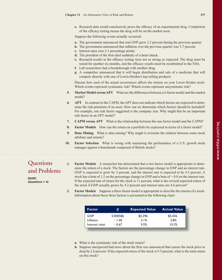
2. Factor Models Suppose a three-factor model is appropriate to describe the returns of a stock. Information about those three factors is presented in the following chart:

a. What is the systematic risk of the stock return?b. Suppose unexpected bad news about the firm was announced that causes the stock price to

drop by 2.6 percent. If the expected return of the stock is 9.5 percent, what is the total return on this stock?

Factor � Expected Value Actual Value

GNP 0.000586 $5,396 $5,436Inflation �1.40 3.1% 3.8%Interest rates �0.67 9.5% 10.3%


ww

w.m

hhe.

com

/rw

j






338 Part III Risk

3. Factors Models Suppose a factor model is appropriate to describe the returns on a stock. The current expected return on the stock is 10.5 percent. Information about those factors is presented in the following chart:

a. What is the systematic risk of the stock return?b. The firm announced that its market share had unexpectedly increased from 23 percent to

27 percent. Investors know from past experience that the stock return will increase by 0.36 percent for every 1 percent increase in its market share. What is the unsystematic risk of the stock?

c. What is the total return on this stock?

4. Multifactor Models Suppose stock returns can be explained by the following three-factor model:

Ri � RF � �1F1 � �2F2 � �3F3

Assume there is no firm-specific risk. The information for each stock is presented here:

The risk premiums for the factors are 5.5 percent, 4.2 percent, and 4.9 percent, respectively. If you create a portfolio with 20 percent invested in stock A, 20 percent invested in stock B, and the remainder in stock C, what is the expression for the return of your portfolio? If the risk-free rate is 5 percent, what is the expected return of your portfolio?

5. Multifactor Models Suppose stock returns can be explained by a two-factor model. The firm-specific risks for all stocks are independent. The following table shows the information for two diversified portfolios:

INTERMEDIATE (Questions 5–7)

�1 �2 E(R)

Portfolio A 0.75 1.20 18%Portfolio B 1.60 �0.20 14

If the risk-free rate is 6 percent, what are the risk premiums for each factor in this model?

6. Market Model The following three stocks are available in the market:

E(R) �

Stock A 10.5% 1.20Stock B 13.0 0.98Stock C 15.7 1.37Market 14.2 1.00

�1 �2 �3

1.20 0.90 0.20 0.80 1.40 �0.30 0.95 �0.05 1.50

Stock AStock BStock C

Factor � Expected Value Actual Value

Growth in GNP 2.04 3.5% 4.8%Inflation �1.90 7.1% 7.8%

ww

w.m

hhe.

com

/rw

j






Assume the market model is valid.a. Write the market model equation for each stock.b. What is the return on a portfolio with weights of 30 percent stock A, 45 percent stock B,

and 25 percent stock C?c. Suppose the return on the market is 15 percent and there are no unsystematic surprises in

the returns. What is the return on each stock? What is the return on the portfolio?

7. Portfolio Risk You are forming an equally weighted portfolio of stocks. Many stocks have the same beta of 0.84 for factor 1 and the same beta of 1.69 for factor 2. All stocks also have the same expected return of 11 percent. Assume a two-factor model describes the return on each of these stocks.a. Write the equation of the returns on your portfolio if you place only five stocks in it.b. Write the equation of the returns on your portfolio if you place in it a very large number of

stocks that all have the same expected returns and the same betas.

8. APT There are two stock markets, each driven by the same common force F with an ex-pected value of zero and standard deviation of 10 percent. There are many securities in each market; thus you can invest in as many stocks as you wish. Due to restrictions, however, you can invest in only one of the two markets. The expected return on every security in both markets is 10 percent.

The returns for each security i in the first market are generated by the relationship

R1i � 0.10 � 1.5F � �1i

where �1i is the term that measures the surprises in the returns of stock i in market l. These surprises are normally distributed; their mean is zero. The returns for security j in the second market are generated by relationship

R2j � 0.10 � 0.5F � �2j

where �2j is the term that measures the surprises in the returns of stock j in market 2. These surprises are normally distributed; their mean is zero. The standard deviation of �1i and �2j for any two stocks, i and j, is 20 percent.a. If the correlation between the surprises in the returns of any two stocks in the first market

is zero, and if the correlation between the surprises in the returns of any two stocks in the second market is zero, in which market would a risk-averse person prefer to invest? (Note: The correlation between �1i and �1j for any i and j is zero, and the correlation between �2i and �2j for any i and j is zero.)

b. If the correlation between �1i and �1j in the first market is 0.9 and the correlation between �2i and �2j in the second market is zero, in which market would a risk-averse person prefer to invest?

c. If the correlation between �1i and �1j in the first market is zero and the correlation between �2i and �2j in the second market is 0.5, in which market would a risk-averse person prefer to invest?

d. In general, what is the relationship between the correlations of the disturbances in the two markets that would make a risk-averse person equally willing to invest in either of the two markets?

9. APT Assume that the following market model adequately describes the return-generating behavior of risky assets:

Rit � �i � �iRMt � �it

Here:

Rit � The return for the ith asset at time t.RMt � The return on a portfolio containing all risky assets in some proportion at time t.RMt and �it are statistically independent.

CHALLENGE (Questions 8–10)


ww

w.m

hhe.

com

/rw

j






340 Part III Risk

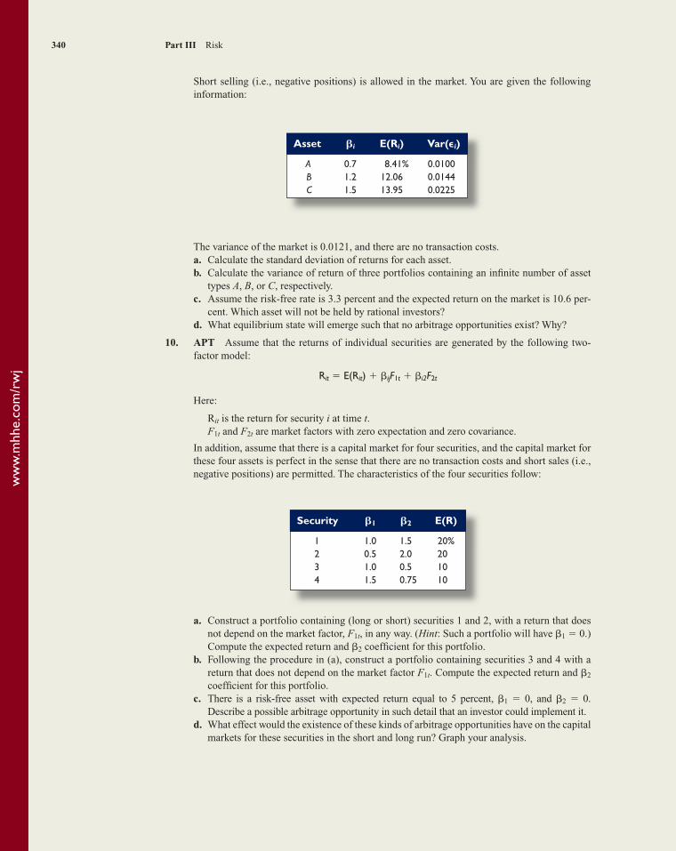
Short selling (i.e., negative positions) is allowed in the market. You are given the following information:

The variance of the market is 0.0121, and there are no transaction costs.a. Calculate the standard deviation of returns for each asset.b. Calculate the variance of return of three portfolios containing an infinite number of asset

types A, B, or C, respectively.c. Assume the risk-free rate is 3.3 percent and the expected return on the market is 10.6 per-

cent. Which asset will not be held by rational investors?d. What equilibrium state will emerge such that no arbitrage opportunities exist? Why?

10. APT Assume that the returns of individual securities are generated by the following two- factor model:

Rit � E(Rit) � �ijF1t � �i2F2t

Here:

Rit is the return for security i at time t. F1t and F2t are market factors with zero expectation and zero covariance.

In addition, assume that there is a capital market for four securities, and the capital market for these four assets is perfect in the sense that there are no transaction costs and short sales (i.e., negative positions) are permitted. The characteristics of the four securities follow:

Asset �i E(Ri) Var(�i)

A 0.7 8.41% 0.0100 B 1.2 12.06 0.0144 C 1.5 13.95 0.0225

a. Construct a portfolio containing (long or short) securities 1 and 2, with a return that does not depend on the market factor, F1t, in any way. (Hint: Such a portfolio will have �1 � 0.) Compute the expected return and �2 coefficient for this portfolio.

b. Following the procedure in (a), construct a portfolio containing securities 3 and 4 with a return that does not depend on the market factor F1t. Compute the expected return and �2 coefficient for this portfolio.

c. There is a risk-free asset with expected return equal to 5 percent, �1 � 0, and �2 � 0. Describe a possible arbitrage opportunity in such detail that an investor could implement it.

d. What effect would the existence of these kinds of arbitrage opportunities have on the capital markets for these securities in the short and long run? Graph your analysis.

Security �1 �2 E(R)

1 1.0 1.5 20% 2 0.5 2.0 20 3 1.0 0.5 10 4 1.5 0.75 10

ww

w.m

hhe.

com

/rw

j






The Fama–French Multifactor Modeland Mutual Fund ReturnsDawn Browne, an investment broker, has been approached by client Jack Thomas about the risk of his investments. Dawn has recently read several articles concerning the risk factors that can potentially affect asset returns, and she has decided to examine Jack’s mutual fund holdings. Jack is currently invested in the Fidelity Magellan Fund (FMAGX), the Fidelity Low-Priced Stock Fund (FLPSX), and the Baron Small Cap Fund (BSCFX). Dawn would like to estimate the well-known multifactor model proposed by Eugene Fama and Ken French to determine the risk of each mutual fund. Here is the regression equation for the multifactor model she proposes to use:

Rit � RFt � �i � �1(RMt � RFt) � �2(SMBt) � �3(HMLt) � �t

In the regression equation, Rit is the return of asset i at time t, RFt is the risk-free rate at time t, and RMt is the return on the market at time t. Thus, the first risk factor in the Fama–French regression is the market factor often used with the CAPM. The second risk factor, SMB or “small minus big,” is calculated by taking the difference in the returns on a portfolio of small-cap stocks and a portfolio of big-cap stocks. This factor is intended to pick up the so-called small firm effect. Similarly, the third factor, HML or “high minus low,” is calculated by taking the difference in the returns between a portfolio of “value” stocks and a portfolio of “growth” stocks. Stocks with low market-to-book ratios are classified as value stocks and vice versa for growth stocks. This factor is included because of the historical tendency for value stocks to earn a higher return. In models such as the one Dawn is considering, the alpha (�) term is of particular interest. It is the regression intercept; but more important, it is also the excess return the asset earned. In other words, if the alpha is positive, the asset earned a return greater than it should have given its level of risk; if the alpha is negative, the asset earned a return lower than it should have given its level of risk. This measure is called “Jensen’s alpha,” and it is a very widely used tool for mutual fund evaluation.

1. For a large-company stock mutual fund, would you expect the betas to be positive or negative for each of the factors in a Fama–French multifactor model?

2. The Fama–French factors and risk-free rates are available at Ken French’s Web site: mba.tuck.dartmouth.edu/pages/faculty/ken.french/. Download the monthly factors and save the most recent 60 months for each factor. The historical prices for each of the mutual funds can be found on various Web sites, including finance.yahoo.com. Find the prices of each mutual fund for the same time as the Fama–French factors and calculate the returns for each month. Be sure to include dividends. For each mutual fund, estimate the multifactor regression equation using the Fama–French factors. How well do the re-gression estimates explain the variation in the return of each mutual fund?

3. What do you observe about the beta coefficients for the different mutual funds? Comment on any similarities or differences.

4. If the market is efficient, what value would you expect for alpha? Do your estimates support market efficiency?

5. Which fund has performed best considering its risk? Why?

Min

i Cas

e

341


chapter 11 an alternative view of risk and returnfinance-agruni.yolasite.com/resources/თავი...

Documents