chapter 11 the ramsey model in use - ku

Chapter 11

The Ramsey model in use

The Ramsey representative agent framework has, rightly or wrongly, been a work-horse for the study of many macroeconomic issues. Among these are public fi-nance themes and themes relating to endogenous productivity growth. In thischapter we consider issues within these two areas. Section 11.1 deals with amarket economy with a public sector. We consider general equilibrium effectsof government spending and taxation. The focus is on effects of shifts in fiscalpolicy and how these effects depend on whether the shift is unanticipated or antic-ipated. In Section 11.2 we set up and analyze a model of technology growth basedon learning by investing. The analysis leads to a characterization of “first-bestpolicy”.

11.1 Fiscal policy and announcement effects

In this section we extend the Ramsey model of a competitive market economy byadding a government sector that spends on goods and services, makes transfersto the private sector, and levies taxes.

Subsection 11.1.1 addresses the effect of government spending on goods andservices, assuming a balanced budget where all taxes are lump sum. One issue iswhat is meant by a one-off policy shock in a context of perfect foresight − soundslike a contradiction. A related issue is how to model the effects of such shocks. Insubsections 11.1.2 and 11.1.3 we consider income taxation and how the economyresponds to the arrival of new information about future fiscal policy. Finally,Subsection 11.1.4 introduces financing by temporary budget deficits. In view ofthe representative agent character of the Ramsey model, it is not surprising thatRicardian equivalence will hold in the model.

443

444 CHAPTER 11. THE RAMSEY MODEL IN USE

11.1.1 Public consumption financed by lump-sum taxes

The representative household (family dynasty) has Lt = L0ent members each

of which supplies one unit of labor inelastically per time unit, n ≥ 0. Thehousehold’s preferences can be represented by a time separable utility function∫ ∞

0

u(ct, Gt)Lte−ρtdt,

where ct ≡ Ct/Lt is consumption per family member andGt is public consumptionin the form of a service delivered by the government, while ρ is the rate of timepreference. We assume, for simplicity, that the instantaneous utility function isadditive: u(c,G) = u(c) + v(G), where u′ > 0, u′′ < 0, i.e., there is positive butdiminishing marginal utility of private consumption; the properties of the utilityfunction v are immaterial for the questions to be studied (but hopefully v′ > 0).The public service consists in making a non-rival good, say “law and order”orTV-transmitted theatre, available for the households free of charge. That theargument of the function v is total Gt, not per capita Gt, is due to the non-rivalcharacter of the public service.Until further notice, the government budget is always balanced. In the present

subsection the government spending, Gt, is financed by a per capita lump-sumtax, τ t, so that

τ tLt = Gt. (11.1)

To allow for balanced growth under technological progress we assume that uis a CRRA function. Thus, the criterion function of the representative householdcan be written

U0 =

∫ ∞0

(c1−θt

1− θ + v(Gt)

)e−(ρ−n)tdt, (11.2)

where θ > 0 is the constant (absolute) elasticity of marginal utility of privateconsumption. For convenience, we assume ρ > 0 throughout.Let the real interest rate and the real wage be denoted rt and wt, respectively.

The household’s dynamic book-keeping equation reads

at = (rt − n)at + wt − τ t − ct, a0 given, (11.3)

where at is per capita financial wealth. The financial wealth is held in claims ofa form similar to a variable-rate deposit in a bank. Hence, at any point in timeat is historically determined and independent of the current and future interestrates. The No-Ponzi-Game condition (solvency condition) is

limt→∞

ate−∫ t0 (rs−n)ds ≥ 0. (NPG)

c© Groth, Lecture notes in macroeconomics, (mimeo) 2016.

11.1. Fiscal policy and announcement effects 445

We see from (11.2) that leisure does not enter the instantaneous utility function.So per capita labor supply is exogenous. We fix it to be one unit of labor pertime unit, as is indicated by (11.3).In view of the additive instantaneous utility function in (11.2), marginal utility

of private consumption is not affected by Gt. The Keynes-Ramsey rule resultingfrom the household’s optimization will therefore be as if there were no governmentsector:

ctct

=1

θ(rt − ρ).

The transversality condition of the household is that (NPG) holds with strictequality, i.e.,

limt→∞

ate−∫ t0 (rs−n)ds = 0.

GDP is produced via an aggregate neoclassical production function with CRS:

Yt = F (Kdt , TtLdt ),

where Kdt and Ldt are inputs of capital and labor, respectively, and Tt is the

technology level, assumed to grow at an exogenous and constant rate g ≥ 0.For simplicity we assume that F satisfies the Inada conditions. It is furtherassumed that in the production of Gt, the same technology (production function)is applied as in the production of the other components of GDP. So the same unitproduction costs are involved. A possible role of Gt for productivity is ignored(so we should not interpret Gt as related to such things as infrastructure, health,education, or research).All capital in the economy is assumed to belong to the private sector. The

economy is closed. In accordance with the standard Ramsey model, there isperfect competition in all markets. Hence there is market clearing so that Kd

t =Kt and Ldt = Lt for all t.

General equilibrium and dynamics

The increase in the capital stock, K, per time unit equals aggregate gross saving:

Kt = Yt−Ct−Gt−δKt = F (Kt, TtLt)−ctLt−Gt−δKt, K0 > 0 given. (11.4)

We assume Gt is proportional to the work force measured in effi ciency units, thatis

Gt = γTtLt, (11.5)

where the size of γ ≥ 0 is decided by the government. The balanced budget(11.1) now implies that the per capita lump-sum tax grows at the same rate astechnology:

τ t = Gt/Lt = γTt = γT0egt = τ 0e

gt. (11.6)



Defining kt ≡ Kt/(TtLt) ≡ kt/Tt and ct ≡ Ct/(TtLt) ≡ ct/Tt, the dynamicaggregate resource constraint (11.4) can be written

·kt = f(kt)− ct − γ − (δ + g + n)kt, k0 > 0 given, (11.7)

where f is the production function in intensive form, f ′ > 0, f ′′ < 0. As F satisfiesthe Inada conditions, f satisfies

f(0) = 0, limk→0

f ′(k) =∞, limk→∞

f ′(k) = 0.

As usual, by the golden-rule capital intensity, kGR, we mean that capitalintensity which maximizes sustainable consumption per unit of effective labor,c+ γ. By setting the left-hand side of (11.7) to zero, eliminating the time indiceson the right-hand side, and rearranging, we get c + γ = f(k) − (δ + g + n)k≡ c(k). In view of the Inada conditions, the problem maxk c(k) has a uniquesolution, k > 0, characterized by the condition f ′(k) = δ + g + n. This k is, bydefinition, kGR.In general equilibrium the real interest rate, rt, equals f ′(kt) − δ. Expressed

in terms of c, the Keynes-Ramsey rule thus becomes

·ct =

1

θ

[f ′(kt)− δ − ρ− θg

]ct. (11.8)

Moreover, we have at = kt ≡ ktTt = ktT0egt, and so the transversality condition

of the representative household can be written

limt→∞

kte−∫ t0 (f ′(ks)−δ−n−g)ds = 0. (11.9)

The phase diagram of the dynamic system (11.7) - (11.8) is shown in Fig. 11.1

where the·k = 0 locus is represented by the stippled inverse-U curve. Apart from

a vertical downward shift of the·k = 0 locus, when we have γ > 0 instead of γ = 0,

the phase diagram is similar to that of the Ramsey model without government.Although the per capita lump-sum tax is not visible in the reduced form of themodel consisting of (11.7), (11.8), and (11.9), it is indirectly present. This is

because it ensures that for all t ≥ 0, the ct and·kt appearing in (11.7) represent

exactly the consumption demand and net saving coming from the households’choices given its intertemporal budget constraint which depends on the lump-sum tax, cf. (11.11) below.We assume γ is of “moderate size” compared to the productive capacity of

the economy so as to not rule out the existence of a steady state. Moreover, to



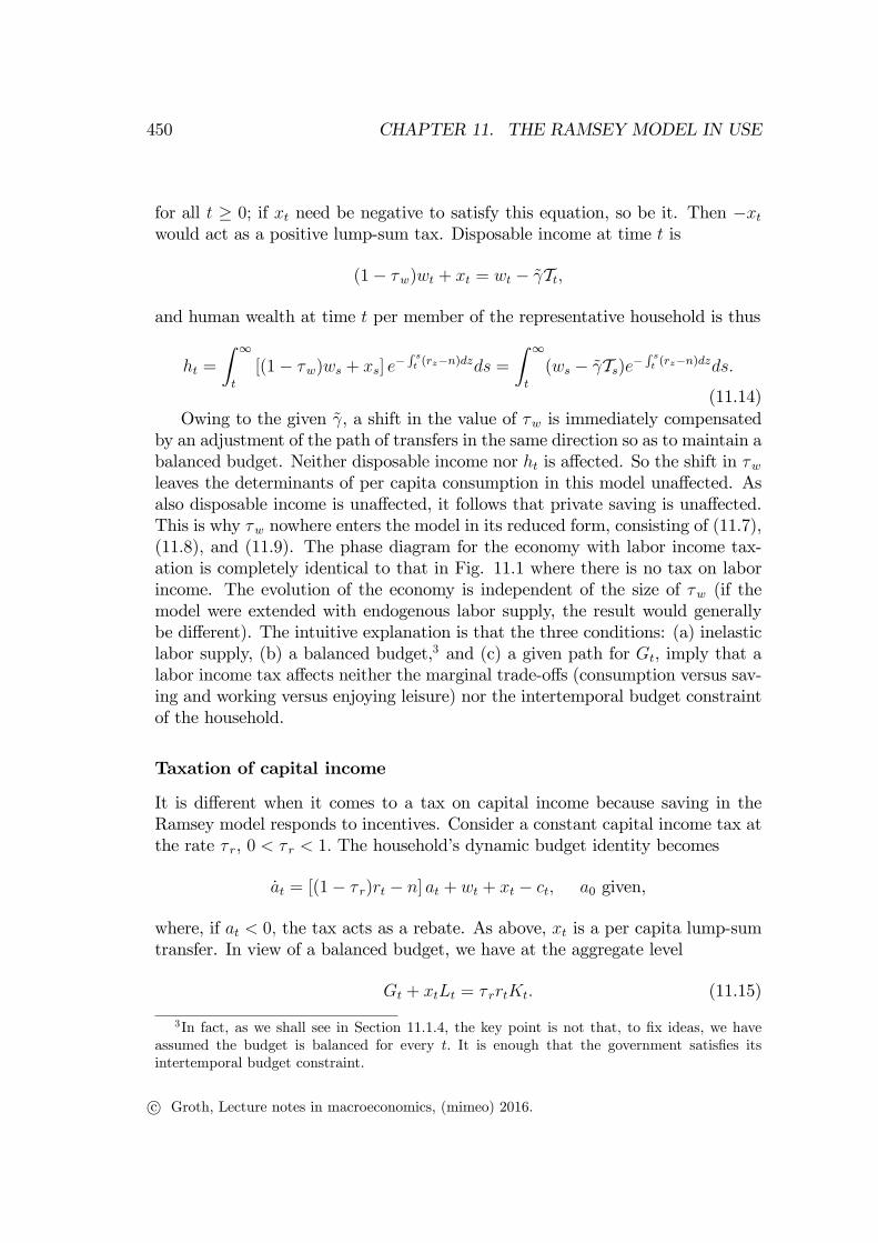
Figure 11.1: Phase portrait of an unanticipated permanent increase in governmentspending from γ to γ′ > γ.

guarantee bounded discounted utility and existence of general equilibrium, weimpose the “suffi cient impatience”restriction

ρ− n > (1− θ)g. (A1)

How to model effects of unanticipated policy shifts

In a perfect foresight model, as the present one, agents’expectations and actionsnever incorporate that unanticipated events, “shocks”, may arrive. That is, ifa shock occurs in historical time, it must be treated as a complete surprise, aone-off shock not expected to be replicated in any sense.Suppose that up until time t0 > 0 government spending maintains the given

ratio Gt/(TtLt) = γ. Suppose further that before time t0, the households expectedthis state of affairs to continue forever. But, unexpectedly, at time t0 there is ashift to a higher constant spending ratio, γ′, which is maintained for a long time.We assume that the upward shift in public spending goes hand in hand with

higher lump-sum taxes so as to maintain a balanced budget. Thereby the after-tax human wealth of the household is at time t0 immediately reduced. As thehouseholds are now less wealthy, cf. (11.11) below, private consumption immedi-ately drops.



Mathematically, the time path of ct will therefore have a discontinuity att = t0. To fix ideas, we will generally consider control variables, e.g., consumption,to be right-continuous functions of time in such cases. This means that ct0 =limt→t+0

ct. Likewise, at such points of discontinuity of the control variable the“time derivative” of the state variable a in (11.3) is generally not well-definedwithout an amendment. In line with the right-continuity of the control variable,we define the time derivative of a state variable at a point of discontinuity of thecontrol variable as the right-hand time derivative, i.e., at0 = limt→t+0

(at−at0)/(t−t0).1 We say that the control variable has a jump at time t0, we call the pointwhere this jump occurs a switch point, and we say that the state variable, whichremains a continuous function of t, has a kink at time t0.In line with this, control variables are called jump variables or forward-looking

variables. The latter name comes from the notion that a decision variable canimmediately shift to another value if new information arrives. In contrast, a statevariable is said to be pre-determined because its value is an outcome of the pastand it cannot jump.

An unanticipated permanent upward shift in government spendingReturning to our specific example, suppose that the economy has been in steadystate for t < t1. Then, unexpectedly, the new spending policy γ′ > γ is intro-duced, followed by an increase in taxation so as to maintain a balanced budget.Let the households rightly expect this new policy to be maintained forever. As a

consequence, the·k = 0 locus in Fig. 11.1 is shifted downwards while the

·c = 0

locus remains where it is. It follows that k stays unchanged at its old steady-state level, k∗, while c jumps down to the new steady-state value, c∗′. There isimmediate crowding out of private consumption to the exact extent of the rise inpublic consumption.2

To understand the mechanism, note that Per capita consumption of the house-hold is

ct = βt(at + ht), (11.10)

where ht is the after-tax human wealth per family member and is given by

ht =

∫ ∞t

(ws − τ s)e−∫ st (rz−n)dzds, (11.11)

1While these conventions help to fix ideas, they are mathematically inconsequential. Indeed,the value of the consumption intensity at each isolated point of discontinuity will affect neitherthe utility integral of the household nor the value of the state variable, a.

2The conclusion is modified, of course, if Gt encompasses public investment and this has animpact on the productivity of the private sector.



and βt is the propensity to consume out of wealth,

βt =1∫∞

te∫ st

((1−θ)rz−ρ

θ+n)dzds

, (11.12)

as derived in the previous chapter. The upward shift in public spending is accom-panied by higher lump-sum taxes, τ ′t = γ′Lt, forever, implying that ht is reduced,which in turn reduces consumption.Had the unanticipated shift in public spending been downward, say from γ′ to

γ, the effect would be an upward jump in consumption but no change in k, thatis, a jump E’to E in Fig. 11.1.Many kinds of disturbances of a steady state will result in a gradual adjust-

ment process, either to a new steady state or back to the original steady state. Itis otherwise in this example where there is an immediate jump to a new steadystate.

11.1.2 Income taxation

We now replace the assumed lump-sum taxation by income taxation of differentkinds. In addition, we introduce lump-sum income transfers to the households.The path of spending on goods and services remains unchanged throughout, i.e.,Gt = γTtLt for all t ≥ 0.

Taxation of labor income

Consider a tax on wage income at the constant rate τw, 0 < τw < 1. Since laborsupply is exogenous, it is unaffected by the wage income tax. While (11.7) isstill the dynamic resource constraint of the economy, the household’s dynamicbook-keeping equation now reads

at = (rt − n)at + (1− τw)wt + xt − ct, a0 given,

where xt is the per capita lump-sum transfers at time t. Maintaining the assump-tion of a balanced budget, the tax revenue at every t exactly covers governmentexpenditure, that is, spending on goods and services plus the lump-sum transfersto the private sector. This means that

τwwtLt = Gt + xtLt for all t ≥ 0. (11.13)

As Gt and τw are given, the interpretation is that for all t ≥ 0, transfers adjustso as to balance the budget. This requires that xt = τwwt−Gt/Lt = τwwt− γTt,



for all t ≥ 0; if xt need be negative to satisfy this equation, so be it. Then −xtwould act as a positive lump-sum tax. Disposable income at time t is

(1− τw)wt + xt = wt − γTt,

and human wealth at time t per member of the representative household is thus

ht =

∫ ∞t

[(1− τw)ws + xs] e−∫ st (rz−n)dzds =

∫ ∞t

(ws − γTs)e−∫ st (rz−n)dzds.

(11.14)Owing to the given γ, a shift in the value of τw is immediately compensated

by an adjustment of the path of transfers in the same direction so as to maintain abalanced budget. Neither disposable income nor ht is affected. So the shift in τwleaves the determinants of per capita consumption in this model unaffected. Asalso disposable income is unaffected, it follows that private saving is unaffected.This is why τw nowhere enters the model in its reduced form, consisting of (11.7),(11.8), and (11.9). The phase diagram for the economy with labor income tax-ation is completely identical to that in Fig. 11.1 where there is no tax on laborincome. The evolution of the economy is independent of the size of τw (if themodel were extended with endogenous labor supply, the result would generallybe different). The intuitive explanation is that the three conditions: (a) inelasticlabor supply, (b) a balanced budget,3 and (c) a given path for Gt, imply that alabor income tax affects neither the marginal trade-offs (consumption versus sav-ing and working versus enjoying leisure) nor the intertemporal budget constraintof the household.

Taxation of capital income

It is different when it comes to a tax on capital income because saving in theRamsey model responds to incentives. Consider a constant capital income tax atthe rate τ r, 0 < τ r < 1. The household’s dynamic budget identity becomes

at = [(1− τ r)rt − n] at + wt + xt − ct, a0 given,

where, if at < 0, the tax acts as a rebate. As above, xt is a per capita lump-sumtransfer. In view of a balanced budget, we have at the aggregate level

Gt + xtLt = τ rrtKt. (11.15)

3In fact, as we shall see in Section 11.1.4, the key point is not that, to fix ideas, we haveassumed the budget is balanced for every t. It is enough that the government satisfies itsintertemporal budget constraint.



As Gt and τ r are given, the interpretation is that for all t ≥ 0, transfers adjustso as to balance the budget. This requires that

xt = τ rrtkt −Gt/Lt = τ rrtkt − γTt. (11.16)

We may rewrite the balanced budget condition (11.15) this way:

τ rrtKt − xtLt = Gt for all t ≥ 0.

We see that as long as the path of Gt is given, so is that of “net taxes”on therepresentative household on the left-hand side. An immediate effect of a changein the tax rate τ r will thus reflect the effect of this change in isolation from anychange in the current net-tax payment as such because there is no such change.Within the model we study: (a) the pure effect on the consumption-saving splitof a change in the tax rate τ r, and (b) the resulting dynamic repercussions in theeconomy as a whole.The No-Ponzi-Game condition of the representative household is

limt→∞

ate−∫ t0 [(1−τr)rs−n]ds ≥ 0,

and the Keynes-Ramsey rule takes the form

ctct

=1

θ[(1− τ r)rt − ρ].

In general equilibrium we have·ct =

1

θ

[(1− τ r)(f ′(kt)− δ)− ρ− θg

]ct. (11.17)

The differential equation for k is still (11.7).In a steady state k∗ satisfies (f ′(k∗)− δ)(1− τ r) = ρ+ θg, that is,

f ′(k∗)− δ =ρ+ θg

1− τ r> ρ+ θg > g + n,

where the last inequality comes from the “suffi cient impatience”assumption (A1).The higher is the tax rate τ r, the lower is k∗. This is implied by f ′′ < 0. Con-sequently, in the long run consumption is lower as well.4 The resulting resourceallocation is not Pareto optimal. There exist an alternative technically feasibleresource allocation that makes everyone in society better off. This is because thecapital income tax implies a wedge between the marginal rate of transformationover time in production, f ′(kt)− δ, and the marginal rate of transformation overtime to which consumers adapt, (1− τ r)(f ′(kt)− δ).

4In the Diamond OLG model a capital income tax, which finances lump-sum transfers to theold generation, has an ambiguous effect on capital accumulation, depending on whether θ < 1or θ > 1, cf. Exercise 5.?? in Chapter 5.



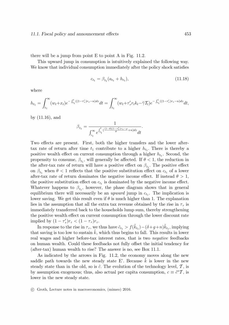
Figure 11.2: Phase portrait of an unanticipated permanent rise in τ r.

11.1.3 Effects of shifts in the capital income tax rate

We shall study effects of a rise in the tax on capital income. The effects dependon whether the change is anticipated in advance or not and whether the change ispermanent or only temporary. So there are four cases to consider. Throughout,the path of spending on goods and services remains unchanged, i.e., Gt = γTtLtfor all t ≥ 0.

(i) Unanticipated permanent upward shift in τ r

Until time t1 the economy has been in steady state with a tax-transfer schemebased on some given constant tax rate, τ r, on capital income. At time t1, unex-pectedly, the government introduces a new tax-transfer scheme, involving a higherconstant tax rate, τ ′r, on capital income, i.e., 0 < τ r < τ ′r < 1. Since the path ofspending on goods and services is unchanged, to maintain a balanced budget, thelump-sum transfers, xt, must be raised. We assume it is credibly announced thatthe new tax-transfer scheme will be adhered to forever. So households expect thereal after-tax interest rate (rate of return on saving) to be (1−τ ′r)rt for all t ≥ t1.For t < t1 the dynamics are governed by (11.7) and (11.17) with 0 < τ r < 1.

The corresponding steady state, E, has k = k∗ and c = c∗ as indicated in thephase diagram in Fig. 11.2. The new tax-transfer scheme ruling after time t1shifts the steady state point to E’with k = k∗′ and c = c∗

′. The new

·c = 0 line

and the new saddle path are to the left of the old, i.e., k∗′ < k∗. Until time t1the economy is at the point E. Immediately after the shift in the tax on capitalincome, equilibrium requires that the economy is on the new saddle path. So



there will be a jump from point E to point A in Fig. 11.2.This upward jump in consumption is intuitively explained the following way.

We know that individual consumption immediately after the policy shock satisfies

ct1 = βt1(at1 + ht1), (11.18)

where

ht1 =

∫ ∞t1

(wt+xt)e−∫ tt1

((1−τ ′r)rz−n)dzdt =

∫ ∞t1

(wt+τ′rrtkt−γTt)e

−∫ tt1

((1−τ ′r)rz−n)dzdt,

by (11.16), and

βt1 =1∫∞

t1e∫ tt1

((1−θ)(1−τ ′r)rz−ρ

θ+n)dz

dt

.

Two effects are present. First, both the higher transfers and the lower after-tax rate of return after time t1 contribute to a higher ht1 . There is thereby apositive wealth effect on current consumption through a higher ht1 . Second, thepropensity to consume, βt1 , will generally be affected. If θ < 1, the reduction inthe after-tax rate of return will have a positive effect on βt1 . The positive effecton βt1 when θ < 1 reflects that the positive substitution effect on ct1 of a lowerafter-tax rate of return dominates the negative income effect. If instead θ > 1,the positive substitution effect on ct1 is dominated by the negative income effect.Whatever happens to βt1 , however, the phase diagram shows that in generalequilibrium there will necessarily be an upward jump in ct1 . The implication islower saving. We get this result even if θ is much higher than 1. The explanationlies in the assumption that all the extra tax revenue obtained by the rise in τ r isimmediately transferred back to the households lump sum, thereby strengtheningthe positive wealth effect on current consumption through the lower discount rateimplied by (1− τ ′r)rz < (1− τ r)rz.In response to the rise in τ r, we thus have ct1 > f(kt1)−(δ+g+n)kt1 , implying

that saving is too low to sustain k, which thus begins to fall. This results in lowerreal wages and higher before-tax interest rates, that is two negative feedbackson human wealth. Could these feedbacks not fully offset the initial tendency for(after-tax) human wealth to rise? The answer is no, see Box 11.1.As indicated by the arrows in Fig. 11.2, the economy moves along the new

saddle path towards the new steady state E’. Because k is lower in the newsteady state than in the old, so is c. The evolution of the technology level, T , isby assumption exogenous; thus, also actual per capita consumption, c ≡ c∗T , islower in the new steady state.



Box 11.1. A mitigating feedback can not instantaneously fully offset theforce that activates it.

Can the story told by Fig. 11.2 be true? Can it be true that the net effect ofthe higher tax on capital income is an upward jump in consumption at timet1 as indicated in Fig. 11.2? Such a jump means that ct1> f(kt1)

−(δ + g + n)kt1 and the resulting reduced saving will make the future k lowerthan otherwise and thereby make expected future real wages lower andexpected future before-tax interest rates higher. Both feedbacks partlycounteract the initial upward shift in human wealth due to higher transfersand a lower effective discount rate that were the direct result of the rise inτw. Could the two mentioned counteracting feedbacks fully offset the initialtendency for (after-tax) human wealth, and therefore current consumption, torise?The phase diagram says no. But what is the intuition? That the two feed-

backs can not fully offset (or even reverse) the tendency for (after-tax) humanwealth to rise at time t1 is explained by the fact that if they could, then the twofeedbacks would not be there in the first place. We cannot at the sametime have both a rise in the human wealth that triggers higher consumption(and thereby lower saving and investment in the economy) and a neutrali-zation, or a complete reversal, of this rise in the human wealth caused bythe higher consumption. The two feedbacks can only partly offset the initialtendency for human wealth to rise.

Instead of all the extra tax revenue obtained being transferred back lump sumto the households, we may alternatively assume that a major part of it is used tofinance a rise in government consumption to the level G′t = γ′TtLt, where γ′ > γ.5

In addition to the leftward shift of the·c = 0 locus this will result in a downward

shift of the·k = 0 locus. The phase diagram would look like a convex combination

of Fig. 11.1 and Fig. 11.2. Then it is possible that the jump in consumption attime t0 becomes downward instead of upward.

Returning to the case where the extra tax revenue is fully transferred, thenext subsection splits the change in taxation policy into two events.

5It is understood that also γ′ is not larger than what allows a steady state to exist. Moreover,the government budget is still balanced for all t so that any temporary surplus or shortage oftax revenue, τ ′rrtKt −G′t, is immediately transferred or levied lump-sum, respectively.



(ii) Anticipated permanent upward shift in τ r

Until time t1 the economy has been in steady state with a tax-transfer schemebased on some given constant tax rate, τ r, on capital income.At time t1, unexpectedly, the government credibly announces that a new fiscal

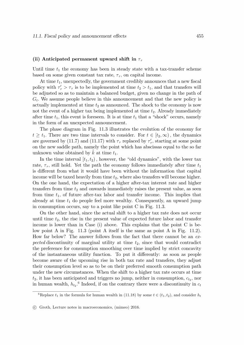
policy with τ ′r > τ r is to be implemented at time t2 > t1, and that transfers willbe adjusted so as to maintain a balanced budget, given no change in the path ofGt. We assume people believe in this announcement and that the new policy isactually implemented at time t2 as announced. The shock to the economy is nownot the event of a higher tax being implemented at time t2. Already immediatelyafter time t1, this event is foreseen. It is at time t1 that a “shock”occurs, namelyin the form of an unexpected announcement.The phase diagram in Fig. 11.3 illustrates the evolution of the economy for

t ≥ t1. There are two time intervals to consider. For t ∈ [t2,∞) , the dynamicsare governed by (11.7) and (11.17) with τ r replaced by τ ′r, starting at some pointon the new saddle path, namely the point which has abscissas equal to the so farunknown value obtained by k at time t1.In the time interval [t1, t2) , however, the “old dynamics”, with the lower tax

rate, τ r, still hold. Yet the path the economy follows immediately after time t1is different from what it would have been without the information that capitalincome will be taxed heavily from time t2, where also transfers will become higher.On the one hand, the expectation of a higher after-tax interest rate and highertransfers from time t2 and onwards immediately raises the present value, as seenfrom time t1, of future after-tax labor and transfer income. This implies thatalready at time t1 do people feel more wealthy. Consequently, an upward jumpin consumption occurs, say to a point like point C in Fig. 11.3.On the other hand, since the actual shift to a higher tax rate does not occur

until time t2, the rise in the present value of expected future labor and transferincome is lower than in Case (i) above. This explains that the point C is be-low point A in Fig. 11.3 (point A itself is the same as point A in Fig. 11.2).How far below? The answer follows from the fact that there cannot be an ex-pected discontinuity of marginal utility at time t2, since that would contradictthe preference for consumption smoothing over time implied by strict concavityof the instantaneous utility function. To put it differently: as soon as peoplebecome aware of the upcoming rise in both tax rate and transfers, they adjusttheir consumption level so as to be on their preferred smooth consumption pathunder the new circumstances. When the shift to a higher tax rate occurs at timet2, it has been anticipated and triggers no jump, neither in consumption, ct2 , norin human wealth, ht2 .

6 Indeed, if on the contrary there were a discontinuity in ct

6Replace t1 in the formula for human wealth in (11.18) by some t ∈ (t1, t2), and consider ht



Figure 11.3: Phase portrait of an anticipated permanent rise in τ r.

at time t2, there would be gains to be obtained by removing this discontinuity.This is due to u′′(c) < 0.

To avoid existence of an expected discontinuity in consumption, the point Con the vertical line k = k∗ in Fig. 11.3 must be such that, following the “olddynamics”, it takes exactly t2− t0 time units to reach the new saddle path. Thisdictates a unique position of the point C between E and A. If C were at a lowerposition, the journey to the saddle path would take longer than t2− t0. And if Cwere at a higher position, the journey would not take as long as t2 − t0.Immediately after time t0, k will be decreasing (because saving is smaller than

what is required to sustain a constant k); and c will be increasing in view of theKeynes-Ramsey rule, since the rate of return on saving is above ρ + θg as longas k < k∗ and τ r low. Precisely at time t2 the economy reaches the new saddlepath, the high taxation of capital income begins, and the after-tax rate of returnbecomes lower than ρ+ θg. Hence, per-capita consumption begins to fall and theeconomy gradually approaches the new steady state E’.This analysis illustrates that when economic agents’ behavior depend on

forward-looking expectations, a credible announcement of a future change in pol-icy has an effect already before the new policy is implemented. Such effects areknown as announcement effects or anticipation effects.As a kind of parallel to our claim that there can be no planned jump in

consumption, consider an asset price. In the asset market arbitrage rules out thepossibility of a generally expected jump in the asset price at a given point in time

as the sum of two integrals, one from t to t2 and one from t2 to∞. Then let t approach t2 frombelow.



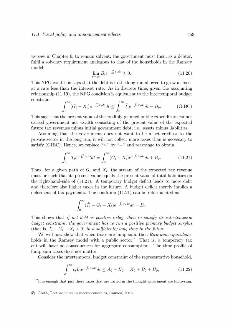
Figure 11.4: Phase portrait of an unanticipated temporary rise in τ r.

in the future. If we imagine the expected jump is upward, an infinite positiverate of return could be obtained by buying the asset immediately before the jump.This would generate excess demand of the asset before time t2 and drive up itsprice in advance thus preventing an expected upward jump to occur at time t2.And if we on the other hand imagine the expected jump is downward, an infinitenegative rate of return could be avoided by selling the asset immediately beforethe jump. This would generate excess supply of the asset before time t2 and driveits price down in advance thus preventing an expected downward jump at t2.In the household’s optimal control problem, cf. Chapter 10.2, the adjoint vari-

able, λ, can be interpreted as a shadow price, and this has some resemblance to anasset price. Recalling the optimality condition u′(ct2) = λt2 , we could also say thatdue to u′′(c) < 0, along an optimal path there can be no expected discontinuity inthe shadow price of financial wealth, λt2 .

(iii) Unanticipated temporary upward shift in τ r

Once again we change the scenario. The economy with low capital taxationhas been in steady state up until time t1. Then a new tax-transfer scheme isunexpectedly introduced. At the same time it is credibly announced that the hightaxes on capital income and the corresponding transfers will cease at time t2 > t1.The path of spending on goods and services remains unchanged throughout, i.e.,Gt = γTtLt for all t ≥ 0.The phase diagram in Fig. 11.4 illustrates the evolution of the economy for

t ≥ t1. For t ≥ t2, the dynamics are governed by (11.7) and (11.17), again withthe old τ r, starting from whatever value obtained by k at time t2.In the time interval [t1, t2) the “new, temporary dynamics”with the high τ ′r



and high transfers hold sway. Yet the path that the economy takes immediatelyafter time t1 is different from what it would have been without the informationthat the new tax-transfers scheme is only temporary. Indeed, the expectation ofa shift to a higher after-tax rate of return and cease of high transfers as of timet2 implies lower present value of expected future labor and transfer earnings thanwithout this information. Hence, the upward jump in consumption at time t1 issmaller than in Fig. 11.2. How much smaller? Again, the answer follows fromthe fact that there can not be an expected discontinuity of marginal utility at timet2, since that would violate the principle of smoothing of planned consumption.Thus the point F on the vertical line k = k∗ in Fig. 11.4 must be such that,following the “new, temporary dynamics”, it takes exactly t2 − t1 time units toreach the solid saddle path in Fig. 11.4 (which is in fact the same as the saddlepath before time t1). The implied position of the economy at time t2 is indicatedby the point G in the figure.Immediately after time t1, k will be decreasing (because saving is smaller than

what is required to sustain a constant k) and c will be decreasing in view of theKeynes-Ramsey rule in a situation with an after-tax rate of return lower thanρ + θg. Precisely at time t2, when the temporary tax-transfers scheme basedon τ ′r is abolished (as announced and expected), the economy reaches the solidsaddle path. From that time the return on saving is high both because of theabolition of the high capital income tax and because k is relatively low. Thegeneral equilibrium effect of this is higher saving, and so the economy movesalong the solid saddle path back to the original steady-state point E.There is a last case to consider, namely an anticipated temporary in τ r. We

leave that for an exercise, see Exercise 11.??

11.1.4 Ricardian equivalence

We now drop the balanced budget assumption and allow public spending to befinanced partly by issuing government bonds and partly by lump-sum taxation.Transfers and gross tax revenue as of time t are called Xt and Tt respectively,while the real value of government net debt is called Bt. Taxes are lump sum. Forsimplicity, we assume all public debt is short-term. Ignoring any money-financingof the spending, the increase per time unit in government debt is identical to thegovernment budget deficit:

Bt = rtBt +Gt +Xt − Tt. (11.19)

As we ignore uncertainty, on its debt the government has to pay the same interestrate, rt, as other borrowers.Because of the “suffi cient impatience”assumption (A1), in the Ramsey model

the long-run interest rate necessarily exceeds the long-run GDP growth rate. As



we saw in Chapter 6, to remain solvent, the government must then, as a debtor,fulfil a solvency requirement analogous to that of the households in the Ramseymodel:

limt→∞

Bte−∫ t0 rsds ≤ 0. (11.20)

This NPG condition says that the debt is in the long run allowed to grow at mostat a rate less than the interest rate. As in discrete time, given the accountingrelationship (11.19), the NPG condition is equivalent to the intertemporal budgetconstraint ∫ ∞

0

(Gt +Xt)e−∫ t0 rsdsdt ≤

∫ ∞0

Tte−∫ t0 rsdsdt−B0. (GIBC)

This says that the present value of the credibly planned public expenditure cannotexceed government net wealth consisting of the present value of the expectedfuture tax revenues minus initial government debt, i.e., assets minus liabilities.Assuming that the government does not want to be a net creditor to the

private sector in the long run, it will not collect more taxes than is necessary tosatisfy (GIBC). Hence, we replace “≤”by “=”and rearrange to obtain∫ ∞

0

Tte−∫ t0 rsdsdt =

∫ ∞0

(Gt +Xt)e−∫ t0 rsdsdt+B0. (11.21)

Thus, for a given path of Gt and Xt, the stream of the expected tax revenuemust be such that its present value equals the present value of total liabilities onthe right-hand-side of (11.21). A temporary budget deficit leads to more debtand therefore also higher taxes in the future. A budget deficit merely implies adeferment of tax payments. The condition (11.21) can be reformulated as∫ ∞

0

(Tt −Gt −Xt)e−∫ t0 rsdsdt = B0.

This shows that if net debt is positive today, then to satisfy its intertemporalbudget constraint, the government has to run a positive primary budget surplus(that is, Tt −Gt −Xt > 0) in a suffi ciently long time in the future.We will now show that when taxes are lump sum, then Ricardian equivalence

holds in the Ramsey model with a public sector.7 That is, a temporary taxcut will have no consequences for aggregate consumption. The time profile oflump-sum taxes does not matter.Consider the intertemporal budget constraint of the representative household,∫ ∞

0

ctLte−∫ t0 rsdsdt ≤ A0 +H0 = K0 +B0 +H0, (11.22)

7It is enough that just those taxes that are varied in the thought experiment are lump-sum.



where H0 is human wealth of the household. This says, that the present value ofthe planned consumption stream can not exceed the total wealth of the household.In the optimal plan of the household, we have strict equality in (11.22).Let τ t denote the lump-sum per capita net tax. Then, Tt −Xt = τ tLt and

H0 = h0L0 =

∫ ∞0

(wt − τ t)Lte−∫ t0 rsdsdt =

∫ ∞0

(wtLt +Xt − Tt)e−∫ t0 rsdsdt

=

∫ ∞0

(wtLt −Gt)e−∫ t0 rsdsdt−B0, (11.23)

where the last equality comes from rearranging (11.21). It follows that

B0 +H0 =

∫ ∞0

(wtLt −Gt)e−∫ t0 rsdsdt.

We see that the time profiles of transfers and taxes have fallen out. What mattersfor total wealth of the forward-looking household is just the spending on goodsand services, not the time profile of transfers and taxes. A higher initial debthas no effect on the sum, B0 + H0, because H0, which incorporates transfersand taxes, becomes equally much lower. Total private wealth is thus unaffectedby government debt. So is therefore also private consumption when net taxesare lump sum. A temporary tax cut will not make people feel wealthier andinduce them to consume more. Instead they will increase their saving by thesame amount as taxes have been reduced, thereby preparing for the higher taxesin the future.This is the Ricardian equivalence result, which we encountered also in Barro’s

discrete time dynasty model in Chapter 7:

In a representative agent model with full employment, rationalexpectations, and no credit market imperfections, if taxes are lumpsum, then, for a given evolution of public expenditure, aggregate pri-vate consumption is independent of whether current public expen-diture is financed by taxes or by issuing bonds. The latter methodmerely implies a deferment of tax payments. Given the government’sintertemporal budget constraint, (11.21), a cut in current taxes hasto be offset by a rise in future taxes of the same present value. Since,with lump-sum taxation, it is only the present value of the stream oftaxes that matters, the “timing”is irrelevant.

Of key importance are the assumption of a representative agent and the as-sumption (A1), leading to a long-run interest rate in excess of the long-run GDPgrowth rate. As pointed out in Chapter 6, Ricardian equivalence breaks down in


11.2. Learning by investing and investment-enhancing policy 461

OLG models without an operative Barro-style bequest motive. Such a bequestmotive is implicit in the infinite horizon of the Ramsey household. In OLG mod-els, where finite life time is emphasized, there is a turnover in the population oftax payers so that taxes levied at different times are levied on partly differentsets of agents. In the future there are newcomers and they will bear part of thehigher future tax burden. Therefore, a current tax cut makes current generationsfeel wealthier and this leads to an increase in current consumption, implying adecrease in national saving, as a result of the temporary deficit finance. Thepresent generations benefit, but future generations bear the cost in the form ofsmaller national wealth than otherwise. We return to further reasons for absenceof Ricardian equivalence in chapters 13 and 19.

11.2 Learning by investing and investment-enhancingpolicy

In endogenous growth theory the Ramsey framework has been applied extensivelyas a simplifying description of the household sector. In most endogenous growththeory the focus is on mechanisms that generate and shape technological change.Different hypotheses about the generation of new technologies are then oftencombined with a simplified picture of the household sector as in the Ramseymodel. Since this results in a simple determination of the long-run interest rate(the modified golden rule), the analyst can in a first approach concentrate on themain issue, technological change, without being disturbed by aspects that areoften secondary to this issue.

As an example, let us consider one of the basic endogenous growth models,the learning-by-investing model, sometimes called the learning-by-doing model.Learning from investment experience and diffusion across firms of the resultingnew technical knowledge (positive externalities) play an important role.

There are two popular alternative versions of the model. The distinguishingfeature is whether the learning parameter (see below) is less than one or equalto one. The first case corresponds to a model by Nobel laureate Kenneth Arrow(1962). The second case has been drawn attention to by Paul Romer (1986) whoassumes that the learning parameter equals one. We first consider the commonframework shared by these two models. Next we describe and analyze Arrow’smodel (in a simplified version) and finally we compare it to Romer’s.



11.2.1 The common framework

We consider a closed economy with firms and households interacting under con-ditions of perfect competition. Later, a government attempting to internalize thepositive investment externality is introduced.Let there be N firms in the economy (N “large”). Suppose they all have

the same neoclassical production function, F, with CRS. Firm no. i faces thetechnology

Yit = F (Kit, TtLit), i = 1, 2, ..., N, (11.24)

where the economy-wide technology level Tt is an increasing function of society’sprevious experience, approximated by cumulative aggregate net investment:

Tt =

(∫ t

−∞Ins ds

)λ= Kλ

t , 0 < λ ≤ 1, (11.25)

where Ins is aggregate net investment and Kt =∑

iKit.8

The idea is that investment − the production of capital goods − as an unin-tended by-product results in experience. The firm and its employees learn fromthis experience. Producers recognize opportunities for process and quality im-provements. In this way knowledge is achieved about how to produce the capitalgoods in a cost-effi cient way and how to design them so that in combinationwith labor they are more productive and satisfy better the needs of the users.Moreover, as emphasized by Arrow,

“each new machine produced and put into use is capable of changingthe environment in which production takes place, so that learning istaking place with continually new stimuli”(Arrow, 1962).9

The learning is assumed to benefit essentially all firms in the economy. Thereare knowledge spillovers across firms and these spillovers are reasonably fast rel-ative to the time horizon relevant for growth theory. In our macroeconomic ap-proach both F and T are in fact assumed to be exactly the same for all firms in theeconomy. That is, in this specification the firms producing consumption-goodsbenefit from the learning just as much as the firms producing capital-goods.The parameter λ indicates the elasticity of the general technology level, T ,

with respect to cumulative aggregate net investment and is named the “learning

8For arbitrary units of measurement for labor and output the hypothesis is Tt = BKλt ,

B > 0. In (11.25) measurement units are chosen such that B = 1.9Concerning empirical evidence of learning-by-doing and learning-by-investing, see Liter-

ature Notes. The citation of Arrow indicates that it was experience from cumulative grossinvestment he had in mind as the basis for learning. Yet, to simplify, we stick to the hypothesisin (11.25), where it is cumulative net investment that matters.



parameter”. Whereas Arrow assumes λ < 1, Romer focuses on the case λ = 1.The case of λ > 1 is ruled out since it would lead to explosive growth (infiniteoutput in finite time) and is therefore not plausible.

The individual firm

In the simple Ramsey model we assumed that households directly own the capitalgoods in the economy and rent them out to the firms. When discussing learning-by-investment, it fits the intuition better if we (realistically) assume that the firmsgenerally own the capital goods they use. They then finance their capital invest-ment by issuing shares and bonds. Households’financial wealth then consists ofthese shares and bonds.Consider firm i. There is perfect competition in all markets. So the firm is

a price taker. Its problem is to choose a production and investment plan whichmaximizes the present value, Vi, of expected future cash-flows. The firm thuschooses (Lit, Iit)

∞t=0 to maximize

Vi0 =

∫ ∞0

[F (Kit, TtLit)− wtLit − Iit] e−∫ t0 rsdsdt

subject to Kit = Iit−δKit. Here wt and It are the real wage and gross investment,respectively, at time t, rs is the real interest rate at time s, and δ ≥ 0 is the capitaldepreciation rate. Rising marginal capital installation costs and other kinds ofadjustment costs are assumed minor and can be ignored. It can be shown, cf.Chapter 14, that in this case the firm’s problem is equivalent to maximization ofcurrent pure profits in every short time interval. So, as hitherto, we can describethe firm as just solving a series of static profit maximization problems.We suppress the time index when not needed for clarity. At any date firm i

maximizes current pure profits, Πi = F (Ki, T Li)− (r+ δ)Ki −wLi, where r+ δis the imputed cost (opportunity cost) per unit of capital used by the firm itself.This leads to the first-order conditions for an interior solution:

∂Πi/∂Ki = F1(Ki, T Li)− (r + δ) = 0, (11.26)

∂Πi/∂Li = F2(Ki, T Li)T − w = 0.

Behind (11.26) is the presumption that each firm is small relative to the economyas a whole, so that each firm’s investment has a negligible effect on the economy-wide technology level Tt. Since F is homogeneous of degree one, by Euler’stheorem,10 the first-order partial derivatives, F1 and F2, are homogeneous ofdegree 0. Thus, we can write (11.26) as

F1(ki, T ) = r + δ, (11.27)

10See Math tools.



where ki ≡ Ki/Li. Since F is neoclassical, F11 < 0. Therefore (11.27) determineski uniquely. From (11.27) follows that the chosen capital-labor ratio, ki, will bethe same for all firms, say k.

The individual household

The household sector is described by our standard Ramsey framework with in-elastic labor supply and a constant population growth rate n ≥ 0. The householdshave CRRA instantaneous utility with parameter θ > 0. The pure rate of timepreference is a constant, ρ. The flow budget identity in per capita terms is

at = (rt − n)at + wt − ct, a0 given,

where a is per capita financial wealth. The NPG condition is

limt→∞

ate−∫ t0 (rs−n)ds ≥ 0.

The resulting consumption-saving plan implies that per capita consumption fol-lows the Keynes-Ramsey rule,

ctct

=1

θ(rt − ρ),

and the transversality condition that the NPG condition is satisfied with strictequality. In general equilibrium of our closed economy with no role for naturalresources and no government debt, at will equal Kt/Lt.

Equilibrium in factor markets

For every t we have in equilibrium that∑

iKi = K and∑

i Li = L, where Kand L are the available amounts of capital and labor, respectively (both pre-determined). Since K =

∑iKi =

∑i kiLi =

∑i kLi = kL, the chosen capital

intensity, ki, satisfies

ki = k =K

L≡ k, i = 1, 2, ..., N. (11.28)

As a consequence we can use (11.27) to determine the equilibrium interest rate:

rt = F1(kt, Tt)− δ. (11.29)

That is, whereas in the firm’s first-order condition (11.27) causality goes from rtto kit, in (11.29) causality goes from kt to rt. Note also that in our closed economywith no natural resources and no government debt, at will equal kt.



The implied aggregate production function is

Y =∑i

Yi ≡∑i

yiLi =∑i

F (ki, T )Li =∑i

F (k, T )Li

= F (k, T )∑i

Li = F (k, T )L = F (K, T L) = F (K,KλL), (11.30)

where we have used (11.24), (11.28), and (11.25) and the assumption that F ishomogeneous of degree one.

11.2.2 The arrow case: λ < 1

The Arrow case is the robust case where the learning parameter satisfies 0 <λ < 1. The method for analyzing the Arrow case is analogue to that used inthe study of the Ramsey model with exogenous technical progress. In particular,aggregate capital per unit of effective labor, k ≡ K/(T L), is a key variable. Lety ≡ Y/(T L). Then

y =F (K, T L)

T L = F (k, 1) ≡ f(k), f ′ > 0, f ′′ < 0. (11.31)

We can now write (11.29) as

rt = f ′(kt)− δ, (11.32)

where kt is pre-determined.

Dynamics

From the definition k ≡ K/(T L) follows

·k

k=

K

K− TT −

L

L=K

K− λK

K− n (by (11.25))

= (1− λ)Y − C − δK

K− n = (1− λ)

y − c− δkk

− n, where c ≡ C

T L ≡c

T .

Multiplying through by k we have

·k = (1− λ)(f(k)− c)− [(1− λ)δ + n] k. (11.33)

In view of (11.32), the Keynes-Ramsey rule implies

gc ≡c

c=

1

θ(r − ρ) =

1

θ

(f ′(k)− δ − ρ

). (11.34)



Defining c ≡ c/A, now follows

.

c

c=

c

c− TT =

c

c− λK

K=c

c− λY − cL− δK

K=c

c− λ

k(y − c− δk)

=1

θ(f ′(k)− δ − ρ)− λ

k(y − c− δk).

Multiplying through by c we have

·c =

[1

θ(f ′(k)− δ − ρ)− λ

k(f(k)− c− δk)

]c. (11.35)

The two coupled differential equations, (11.33) and (11.35), determine theevolution over time of the economy.

Phase diagram Fig. 11.5 depicts the phase diagram. The·k = 0 locus comes

from (11.33), which gives

·k = 0 for c = f(k)− (δ +

n

1− λ)k, (11.36)

where we realistically may assume that δ + n/(1− λ) > 0. As to the·c = 0 locus,

we have

·c = 0 for c = f(k)− δk − k

λθ(f ′(k)− δ − ρ)

= f(k)− δk − k

λgc ≡ c(k) (from (11.34)). (11.37)

Before determining the slope of the·c = 0 locus, it is convenient to consider

the steady state, (k∗, c∗).

Steady state In a steady state c and k are constant so that the growth rate ofC as well as K equals A/A+ n, i.e.,

C

C=K

K=TT + n = λ

K

K+ n.

Solving givesC

C=K

K=

n

1− λ.



Figure 11.5: Phase diagram for the Arrow model.

Thence, in a steady state

gc =C

C− n =

n

1− λ − n =λn

1− λ ≡ g∗c , and (11.38)

TT = λ

K

K=

λn

1− λ = g∗c . (11.39)

The steady-state values of r and k, respectively, will therefore satisfy, by (11.34),

r∗ = f ′(k∗)− δ = ρ+ θg∗c = ρ+ θλn

1− λ. (11.40)

To ensure existence of a steady state we assume that the private marginal pro-ductivity of capital is suffi ciently sensitive to capital per unit of effective labor,from now called the “capital intensity”:

limk→0

f ′(k) > δ + ρ+ θλn

1− λ > limk→∞

f ′(k). (A1)

The transversality condition of the representative household is that limt→∞ate−∫ t0 (rs−n)ds = 0, where at is per capita financial wealth. In general equilibrium



at = kt ≡ ktTt, where Tt in steady state grows according to (11.39). Thus, insteady state the transversality condition can be written

limt→∞

k∗e(g∗c−r∗+n)t = 0. (TVC)

For this to hold, we need

r∗ > g∗c + n =n

1− λ, (11.41)

by (11.38). In view of (11.40), this is equivalent to

ρ− n > (1− θ) λn

1− λ, (A2)

which we assume satisfied.As to the slope of the

·c = 0 locus we have from (11.37),

c′(k) = f ′(k)− δ − 1

λ(kf ′′(k)

θ+ gc) > f ′(k)− δ − 1

λgc, (11.42)

since f ′′ < 0. At least in a small neighborhood of the steady state we can signthe right-hand side of this expression. Indeed,

f ′(k∗)−δ− 1

λg∗c = ρ+θg∗c−

1

λg∗c = ρ+θ

λn

1− λ−n

1− λ = ρ−n−(1−θ) λn

1− λ > 0,

(11.43)by (11.38) and (A2). So, combining with (11.42), we conclude that c′(k∗) > 0.By continuity, in a small neighborhood of the steady state, c′(k) ≈ c′(k∗) > 0.

Therefore, close to the steady state, the·c = 0 locus is positively sloped, as

indicated in Fig. 11.5.Still, we have to check the following question: In a neighborhood of the steady

state, which is steeper, the·c = 0 locus or the

·k = 0 locus? The slope of the latter

is f ′(k)− δ − n/(1− λ), from (11.36). At the steady state this slope is

f ′(k∗)− δ − 1

λg∗c ∈ (0, c′(k∗)),

in view of (11.43) and (11.42). The·c = 0 locus is thus steeper. So, the

·c = 0

locus crosses the·k = 0 locus from below and can only cross once.

The assumption (A1) ensures existence of a k∗ > 0 satisfying (11.40). AsFig. 11.5 is drawn, a little more is implicitly assumed namely that there exists a



k > 0 such that the private net marginal productivity of capital equals the thesteady-state growth rate of output, i.e.,

f ′(k)− δ = (Y

Y)∗ = (

TT )∗ +

L

L=

λn

1− λ + n =n

1− λ, (11.44)

where we have used (11.39). Thus, the tangent to the·k = 0 locus at k = k is

horizontal and k > k∗ as indicated in the figure.Note, however, that k is not the golden-rule capital intensity. The latter is the

capital intensity, kGR, at which the social net marginal productivity of capitalequals the steady-state growth rate of output (see Appendix). If kGR exists, it willbe larger than k as indicated in Fig. 11.5. To see this, we now derive a convenientexpression for the social marginal productivity of capital. From (11.30) we have

∂Y

∂K= F1(·) + F2(·)λKλ−1L = f ′(k) + F2(·)KλL(λK−1) (by (11.31))

= f ′(k) + (F (·)− F1(·)K)λK−1 (by Euler’s theorem)

= f ′(k) + (f(k)KλL− f ′(k)K)λK−1 (by (11.31) and (11.25))

= f ′(k) + (f(k)Kλ−1L− f ′(k))λ = f ′(k) + λf(k)− kf ′(k)

k> f ′(k).

in view of k = K/(KλL) = K1−λL−1 and f(k)/k − f ′(k) > 0. As expected, thepositive externality makes the social marginal productivity of capital larger thanthe private one. Since we can also write ∂Y/∂K = (1−λ)f ′(k)+λf(k)/k, we seethat ∂Y/∂K is a decreasing function of k (both f ′(k) and f(k)/k are decreasingin k.Now, the golden-rule capital intensity, kGR, will be that capital intensity which

satisfies

f ′(kGR) + λf(kGR)− kGRf ′(kGR)

kGR− δ = (

Y

Y)∗ =

n

1− λ.

To ensure there exists such a kGR, we strengthen the right-hand side inequalityin (A1) by the assumption

limk→∞

(f ′(k) + λ

f(k)− kf ′(k)

k

)< δ +

n

1− λ. (A3)

This, together with (A1) and f′′< 0, implies existence of a unique kGR, and in

view of our additional assumption (A2), we have 0 < k∗ < k < kGR, as displayedin Fig. 11.5.



Stability The arrows in Fig. 11.5 indicate the direction of movement as de-termined by (11.33) and (11.35). We see that the steady state is a saddle point.The dynamic system has one pre-determined variable, k, and one jump variable,c. The saddle path is not parallel to the jump variable axis. We claim that fora given k0 > 0, (i) the initial value of c0 will be the ordinate to the point wherethe vertical line k = k0 crosses the saddle path; (ii) over time the economy willmove along the saddle path towards the steady state. Indeed, this time path isconsistent with all conditions of general equilibrium, including the transversalitycondition (TVC). And the path is the only technically feasible path with thisproperty. Indeed, all the divergent paths in Fig. 11.5 can be ruled out as equi-librium paths because they can be shown to violate the transversality conditionof the household.In the long run c and y ≡ Y/L ≡ yT = f(k∗)T grow at the rate λn/(1− λ),

which is positive if and only if n > 0. This is an example of endogenous growth inthe sense that the positive long-run per capita growth rate is generated through aninternal mechanism (learning) in the model (in contrast to exogenous technologygrowth as in the Ramsey model with exogenous technical progress).

Two types of endogenous growth

One may distinguish between two types of endogenous growth. One is called fullyendogenous growth which occurs when the long-run growth rate of c is positivewithout the support by growth in any exogenous factor (for example exogenousgrowth in the labor force); the Romer case, to be considered in the next section,provides an example. The other type is called semi-endogenous growth and ispresent if growth is endogenous but a positive per capita growth rate can not bemaintained in the long run without the support by growth in some exogenousfactor (for example growth in the labor force). Clearly, in the Arrow model oflearning by investing, growth is “only” semi-endogenous. The technical reasonfor this is the assumption that the learning parameter λ is below 1, which impliesdiminishing returns to capital at the aggregate level. If and only if n > 0, do wehave c/c > 0 in the long run.11 In line with this, ∂g∗y/∂n > 0.The key role of population growth derives from the fact that although there

are diminishing marginal returns to capital at the aggregate level, there are in-creasing returns to scale w.r.t. capital and labor. For the increasing returns tobe exploited, growth in the labor force is needed. To put it differently: whenthere are increasing returns to K and L together, growth in the labor force notonly counterbalances the falling marginal productivity of aggregate capital (this

11Note, however, that the model, and therefore (11.38), presupposes n ≥ 0. If n < 0, thenK would tend to be decreasing and so, by (11.25), the level of technical knowledge would bedecreasing, which is implausible, at least for a modern industrialized economy.



counter-balancing role reflects the complementarity between K and L), but alsoupholds sustained productivity growth.Note that in the semi-endogenous growth case ∂g∗y/∂λ = n/(1 − λ)2 > 0 for

n > 0. That is, a higher value of the learning parameter implies higher per capitagrowth in the long run, when n > 0. Note also that ∂g∗y/∂ρ = 0 = ∂g∗y/∂θ, thatis, in the semi-endogenous growth case preference parameters do not matter forlong-run growth. As indicated by (11.38), the long-run growth rate is tied downby the learning parameter, λ, and the rate of population growth, n. But, like inthe simple Ramsey model, it can be shown that preference parameters matter forthe level of the growth path. This suggests that taxes and subsidies do not havelong-run growth effects, but “only” level effects (see Exercise 11.??).

11.2.3 Romer’s limiting case: λ = 1, n = 0

We now consider the limiting case λ = 1. We should think of it as a thoughtexperiment because, by most observers, the value 1 is considered an unrealisticallyhigh value for the learning parameter. To avoid a forever rising growth rate wehave to add the restriction n = 0.

The resulting model turns out to be extremely simple and at the same timeit gives striking results (both circumstances have probably contributed to itspopularity).First, with λ = 1 we get T = K and so the equilibrium interest rate is, by

(11.29),

r = F1(k,K)− δ = F1(1, L)− δ ≡ r,

where we have divided the two arguments of F1(k,K) by k ≡ K/L and againused Euler’s theorem. Note that the interest rate is constant “from the beginning”and independent of the historically given initial value of K, K0. The aggregateproduction function is now

Y = F (K,KL) = F (1, L)K, L constant, (11.45)

and is thus linear in the aggregate capital stock. In this way the general neo-classical presumption of diminishing returns to capital has been suspended andreplaced by exactly constant returns to capital. So the Romer model belongs to aclass of models known as AK models, that is, models where in general equilibriumthe interest rate and the output-capital ratio are necessarily constant over timewhatever the initial conditions.The method for analyzing an AK model is different from the one used for a

diminishing returns model as above.



Dynamics

The Keynes-Ramsey rule now takes the form

c

c=

1

θ(r − ρ) =

1

θ(F1(1, L)− δ − ρ) ≡ γ, (11.46)

which is also constant “from the beginning”. To ensure positive growth, weassume

F1(1, L)− δ > ρ. (A1’)

And to ensure bounded intertemporal utility (and existence of equilibrium), it isassumed that

ρ > (1− θ)γ and therefore γ < θγ + ρ = r. (A2’)

Solving the linear differential equation (11.46) gives

ct = c0eγt, (11.47)

where c0 is unknown so far (because c is not a predetermined variable). We shallfind c0 by applying the households’transversality condition

limt→∞

ate−rt = lim

t→∞kte−rt = 0. (TVC)

First, note that the dynamic resource constraint for the economy is

K = Y − cL− δK = F (1, L)K − cL− δK,

or, in per-capita terms,

k = [F (1, L)− δ] k − c0eγt. (11.48)

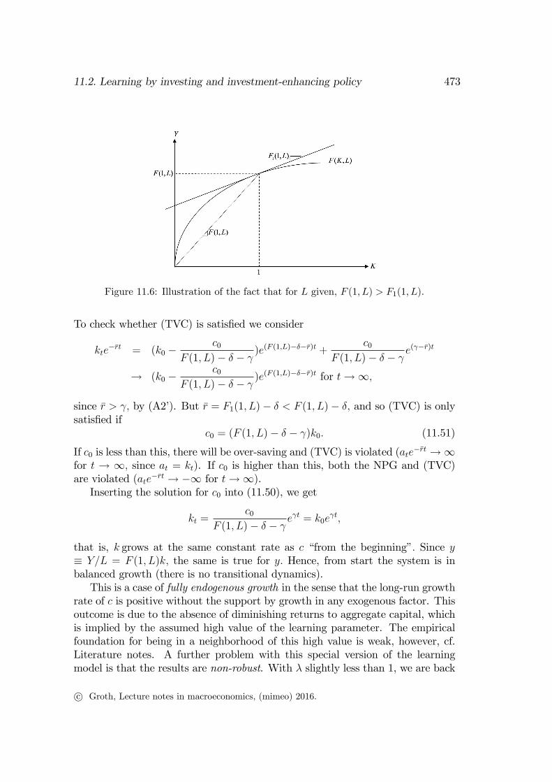
In this equation it is important that F (1, L) − δ − γ > 0. To understand thisinequality, note that, by (A2’), F (1, L)−δ−γ > F (1, L)−δ−r = F (1, L)−F1(1, L)= F2(1, L)L > 0, where the first equality is due to r = F1(1, L)−δ and the secondis due to the fact that since F is homogeneous of degree 1, we have, by Euler’stheorem, F (1, L) = F1(1, L) · 1 +F2(1, L)L > F1(1, L) > δ, in view of (A1’). Thekey property F (1, L)− F1(1, L) > 0 is illustrated in Fig. 11.6.The solution of a linear differential equation of the form x(t) + ax(t) = ceht,

with h 6= −a, isx(t) = (x(0)− c

a+ h)e−at +

c

a+ heht. (11.49)

Thus the solution to (11.48) is

kt = (k0 −c0

F (1, L)− δ − γ )e(F (1,L)−δ)t +c0

F (1, L)− δ − γ eγt. (11.50)



Figure 11.6: Illustration of the fact that for L given, F (1, L) > F1(1, L).

To check whether (TVC) is satisfied we consider

kte−rt = (k0 −

c0

F (1, L)− δ − γ )e(F (1,L)−δ−r)t +c0

F (1, L)− δ − γ e(γ−r)t

→ (k0 −c0

F (1, L)− δ − γ )e(F (1,L)−δ−r)t for t→∞,

since r > γ, by (A2’). But r = F1(1, L)− δ < F (1, L)− δ, and so (TVC) is onlysatisfied if

c0 = (F (1, L)− δ − γ)k0. (11.51)

If c0 is less than this, there will be over-saving and (TVC) is violated (ate−rt →∞for t → ∞, since at = kt). If c0 is higher than this, both the NPG and (TVC)are violated (ate

−rt → −∞ for t→∞).Inserting the solution for c0 into (11.50), we get

kt =c0

F (1, L)− δ − γ eγt = k0e

γt,

that is, k grows at the same constant rate as c “from the beginning”. Since y≡ Y/L = F (1, L)k, the same is true for y. Hence, from start the system is inbalanced growth (there is no transitional dynamics).This is a case of fully endogenous growth in the sense that the long-run growth

rate of c is positive without the support by growth in any exogenous factor. Thisoutcome is due to the absence of diminishing returns to aggregate capital, whichis implied by the assumed high value of the learning parameter. The empiricalfoundation for being in a neighborhood of this high value is weak, however, cf.Literature notes. A further problem with this special version of the learningmodel is that the results are non-robust. With λ slightly less than 1, we are back



in the Arrow case and growth peters out, since n = 0.With λ slightly above 1, itcan be shown that growth becomes explosive (infinite output in finite time).12

The Romer case, λ = 1, is thus a knife-edge case in a double sense. First,it imposes a particular value for a parameter which apriori can take any valuewithin an interval. Second, the imposed value leads to theoretically non-robustresults; values in a hair’s breadth distance result in qualitatively different behaviorof the dynamic system. Still, whether the Romer case - or, more generally, afully-endogenous growth case - can be used as an empirical approximation toits semi-endogenous “counterpart” for a suffi ciently long time horizon to be ofinterest, is a debated question within growth analysis.It is noteworthy that the causal structure in the long run in the diminishing

returns case is different than in the AK-case of Romer. In the diminishing returnscase the steady-state growth rate is determined first, as g∗c in (11.38), and then r

∗

is determined through the Keynes-Ramsey rule; finally, Y/K is determined by thetechnology, given r∗. In contrast, the Romer case has Y/K and r directly givenas F (1, L) and r, respectively. In turn, r determines the (constant) equilibriumgrowth rate through the Keynes-Ramsey rule.

Economic policy in the Romer case

In the AK case, that is, the fully endogenous growth case, we have ∂γ/∂ρ < 0 and∂γ/∂θ < 0. Thus, preference parameters matter for the long-run growth rate andnot “only”for the level of the growth path. This suggests that taxes and subsidiescan have long-run growth effects. In any case, in this model there is a motivationfor government intervention due to the positive externality of private investment.This motivation is present whether λ < 1 or λ = 1. Here we concentrate on thelatter case, which is the simpler one. We first find the social planner’s solution.

The social planner The social planner faces the aggregate production functionYt = F (1, L)Kt or, in per capita terms, yt = F (1, L)kt. The social planner’sproblem is to choose (ct)

∞=0 to maximize

U0 =

∫ ∞0

c1−θt

1− θe−ρtdt s.t.

ct ≥ 0,

kt = F (1, L)kt − ct − δkt, k0 > 0 given, (11.52)

kt ≥ 0 for all t > 0. (11.53)

12See Solow (1997).



The current-value Hamiltonian is

H(k, c, η, t) =c1−θ

1− θ + η (F (1, L)k − c− δk) ,

where η = ηt is the adjoint variable associated with the state variable, which iscapital per unit of labor. Necessary first-order conditions for an interior optimalsolution are

∂H

∂c= c−θ − η = 0, i.e., c−θ = η, (11.54)

∂H

∂k= η(F (1, L)− δ) = −η + ρη. (11.55)

We guess that also the transversality condition,

limt→∞

ktηte−ρt = 0, (11.56)

must be satisfied by an optimal solution. This guess will be of help in finding acandidate solution. Having found a candidate solution, we shall invoke a theoremon suffi cient conditions to ensure that our candidate solution is really a solution.Log-differentiating w.r.t. t in (11.54) and combining with (11.55) gives the

social planner’s Keynes-Ramsey rule,

ctct

=1

θ(F (1, L)− δ − ρ) ≡ γSP . (11.57)

We see that γSP > γ. This is because the social planner internalizes the economy-wide learning effect associated with capital investment, that is, the social plannertakes into account that the “social”marginal productivity of capital is ∂yt/∂kt= F (1, L) > F1(1, L). To ensure bounded intertemporal utility we sharpen (A2’)to

ρ > (1− θ)γSP . (A2”)

To find the time path of kt, note that the dynamic resource constraint (11.52)can be written

kt = (F (1, L)− δ)kt − c0eγSP t,

in view of (11.57). By the general solution formula (11.49) this has the solution

kt = (k0 −c0

F (1, L)− δ − γSP)e(F (1,L)−δ)t +

c0

F (1, L)− δ − γSPeγSP t. (11.58)

In view of (11.55), in an interior optimal solution the time path of the adjointvariable η is

ηt = η0e−[(F (1,L)−δ−ρ]t,



where η0 = c−θ0 > 0, by (11.54). Thus, the conjectured transversality condition(11.56) implies

limt→∞

kte−(F (1,L)−δ)t = 0, (11.59)

where we have eliminated η0. To ensure that this is satisfied, we multiply kt from(11.58) by e−(F (1,L)−δ)t to get

kte−(F (1,L)−δ)t = k0 −

c0

F (1, L)− δ − γSP+

c0

F (1, L)− δ − γSPe[γSP−(F (1,L)−δ)]t

→ k0 −c0

F (1, L)− δ − γSPfor t→∞,

since, by (A2”), γSP < ρ+ θγSP = F (1, L)− δ in view of (11.57). Thus, (11.59)is only satisfied if

c0 = (F (1, L)− δ − γSP )k0. (11.60)

Inserting this solution for c0 into (11.58), we get

kt =c0

F (1, L)− δ − γSPeγSP t = k0e

γSP t,

that is, k grows at the same constant rate as c “from the beginning”. Since y≡ Y/L = F (1, L)k, the same is true for y. Hence, our candidate for the so-cial planner’s solution is from start in balanced growth (there is no transitionaldynamics).The next step is to check whether our candidate solution satisfies a set of

suffi cient conditions for an optimal solution. Here we can use Mangasarian’stheorem. Applied to a continuous-time optimization problem like this, with onecontrol variable and one state variable, the theorem says that the following con-ditions are suffi cient:

(a) Concavity: For all t ≥ 0 the Hamiltonian is jointly concave in the controland state variables, here c and k.

(b) Non-negativity: There is for all t ≥ 0 a non-negativity constraint on thestate variable; in addition, the co-state variable, η, is non-negative for allt ≥ 0 along the optimal path.

(c) TVC: The candidate solution satisfies the transversality conditionlimt→∞ ktηte

−ρt = 0, where ηte−ρt is the discounted co-state variable.

In the present case we see that the Hamiltonian is a sum of concave func-tions and therefore is itself concave in (k, c). Further, from (11.53) we see thatcondition (b) is satisfied. Finally, our candidate solution is constructed so as tosatisfy condition (c). The conclusion is that our candidate solution is an optimalsolution. We call it an SP allocation.



Implementing the SP allocation in the market economy Returning tothe competitive market economy, we assume there is a policy maker, the govern-ment, with only two activities. These are (i) paying an investment subsidy, s, tothe firms so that their capital costs are reduced to

(1− s)(r + δ)

per unit of capital per time unit; (ii) financing this subsidy by a constant con-sumption tax rate τ .Let us first find the size of s needed to establish the SP allocation. Firm i

now chooses Ki such that

∂Yi∂Ki

|K fixed = F1(Ki, KLi) = (1− s)(r + δ).

By Euler’s theorem this implies

F1(ki, K) = (1− s)(r + δ) for all i,

so that in equilibrium we must have

F1(k,K) = (1− s)(r + δ),

where k ≡ K/L, which is pre-determined from the supply side. Thus, the equi-librium interest rate must satisfy

r =F1(k,K)

1− s − δ =F1(1, L)

1− s − δ, (11.61)

again using Euler’s theorem.It follows that s should be chosen such that the “right” r arises. What is

the “right” r? It is that net rate of return which is implied by the productiontechnology at the aggregate level, namely ∂Y/∂K − δ = F (1, L) − δ. If we canobtain r = F (1, L)− δ, then there is no wedge between the intertemporal rate oftransformation faced by the consumer and that implied by the technology. Therequired s thus satisfies

r =F1(1, L)

1− s − δ = F (1, L)− δ,

so that

s = 1− F1(1, L)

F (1, L)=F (1, L)− F1(1, L)

F (1, L)=F2(1, L)L

F (1, L).



It remains to find the required consumption tax rate τ . The tax revenue willbe τcL, and the required tax revenue is

T = s(r + δ)K = (F (1, L)− F1(1, L))K = τcL.

Thus, with a balanced budget the required tax rate is

τ =TcL

=F (1, L)− F1(1, L)

c/k=F (1, L)− F1(1, L)

F (1, L)− δ − γSP> 0, (11.62)

where we have used that the proportionality in (11.60) between c and k holds forall t ≥ 0. Substituting (11.57) into (11.62), the solution for τ can be written

τ =θ [F (1, L)− F1(1, L)]

(θ − 1)(F (1, L)− δ) + ρ=

θF2(1, L)L

(θ − 1)(F (1, L)− δ) + ρ.

The required tax rate on consumption is thus a constant. It therefore does notdistort the consumption/saving decision on the margin, cf. Appendix B.It follows that the allocation obtained by this subsidy-tax policy is the SP

allocation. A policy, here the policy (s, τ), which in a decentralized system in-duces the SP allocation, is called a first-best policy. In a situation where for somereason it is impossible to obtain an SP allocation in a decentralized way (becauseof adverse selection and moral hazard problems, say), a government’s optimiza-tion problem would involve additional constraints to those given by technologyand initial resources. A decentralized implementation of the solution to such aproblem is called a second-best policy.

11.3 Concluding remarks

(not yet available)

11.4 Literature notes

(incomplete)As to empirical evidence of learning-by-doing and learning-by-investing, see

...As noted in Section 11.2.1, the citation of Arrow indicates that it was expe-

rience from cumulative gross investment, rather than net investment, he had inmind as the basis for learning. Yet the hypothesis in (11.25) is the more popu-lar one - seemingly for no better reason than that it leads to simpler dynamics.


11.5. Appendix 479

Another way in which (11.25) deviates from Arrow’s original ideas is by assum-ing that technical progress is disembodied rather than embodied, a distinction wetouched upon in Chapter 2. Moreover, we have assumed a neoclassical technologywhereas Arrow assumed fixed technical coeffi cients.

11.5 Appendix

A. The golden-rule capital intensity in Arrow’s growth model

In our discussion of Arrow’s learning-by-investing model in Section 11.2.2 (where0 < λ < 1), we claimed that the golden-rule capital intensity, kGR, will be that ef-fective capital-labor ratio at which the social net marginal productivity of capitalequals the steady-state growth rate of output. In this respect the Arrow modelwith endogenous technical progress is similar to the standard neoclassical growthmodel with exogenous technical progress. This claim corresponds to a very gen-eral theorem, valid also for models with many capital goods and non-existence ofan aggregate production function. This theorem says that the highest sustainablepath for consumption per unit of labor in the economy will be that path whichresults from those techniques which profit maximizing firms choose under perfectcompetition when the real interest rate equals the steady-state growth rate ofGNP (see Gale and Rockwell, 1975).To prove our claim, note that in steady state, (11.37) holds whereby consump-

tion per unit of labor (here the same as per capita consumption as L = laborforce = population) can be written

ct ≡ ctTt =

[f(k)− (δ +

n

1− λ)k

]Kλt

=

[f(k)− (δ +

n

1− λ)k

](K0e

n1−λ t)λ

(by g∗K =n

1− λ)

=

[f(k)− (δ +

n

1− λ)k

]((kL0)

11−λ e

n1−λ t)λ

(from k =Kt

Kλt Lt

=K1−λ

0

L0

)

=

[f(k)− (δ +

n

1− λ)k

]k

λ1−λL0

λ1−λ e

λn1−λ t ≡ ϕ(k)L0

λ1−λ e

λn1−λ t,

defining ϕ(k) in the obvious way.We look for that value of k at which this steady-state path for ct is at the

highest technically feasible level. The positive coeffi cient, L0

λ1−λ e

λn1−λ t, is the only

time dependent factor and can be ignored since it is exogenous. The problem isthereby reduced to the static problem of maximizing ϕ(k) with respect to k > 0.



We find

ϕ′(k) =

[f ′(k)− (δ +

n

1− λ)

]k

λ1−λ +

[f(k)− (δ +

n

1− λ)k

]λ

1− λkλ

1−λ−1

=

[f ′(k)− (δ +

n

1− λ) +

(f(k)

k− (δ +

n

1− λ)

)λ

1− λ

]k

λ1−λ

=

[(1− λ)f ′(k)− (1− λ)δ − n+ λ

f(k)

k− λ(δ +

n

1− λ)

]k

λ1−λ

1− λ

=

[(1− λ)f ′(k)− δ + λ

f(k)

k− n

1− λ

]k

λ1−λ

1− λ ≡ ψ(k)k

λ1−λ

1− λ, (11.63)

defining ψ(k) in the obvious way. The first-order condition for the problem,ϕ′(k) = 0, is equivalent to ψ(k) = 0. After ordering this gives

f ′(k) + λf(k)− kf ′(k)

k− δ =

n

1− λ. (11.64)

We see thatϕ′(k) R 0 for ψ(k) R 0,

respectively. Moreover,

ψ′(k) = (1− λ)f ′′(k)− λf(k)− kf ′(k)

k2< 0,

in view of f ′′ < 0 and f(k)/k > f ′(k). So a k > 0 satisfying ψ(k) = 0 is theunique maximizer of ϕ(k). By (A1) and (A3) in Section 11.2.2 such a k existsand is thereby the same as the kGR we were looking for.The left-hand side of (11.64) equals the social marginal productivity of capital

and the right-hand side equals the steady-state growth rate of output. At k = kGRit therefore holds that

∂Y

∂K− δ =

(Y

Y

)∗.

This confirms our claim in Section 11.2.2 about kGR.

Remark about the absence of a golden rule in the Romer case. In the Romer casethe golden rule is not a well-defined concept for the following reason. Along anybalanced growth path we have from (11.52),

gk ≡ktkt

= F (1, L)− δ − ctkt

= F (1, L)− δ − c0

k0

,


11.5. Appendix 481

because gk (= gK) is by definition constant along a balanced growth path, wherebyalso ct/kt must be constant. We see that gk is decreasing linearly from F (1, L)−δto −δ when c0/k0 rises from nil to F (1, L). So choosing among alternative techni-cally feasible balanced growth paths is inevitably a choice between starting withlow consumption to get high growth forever or starting with high consumptionto get low growth forever. Given any k0 > 0, the alternative possible balancedgrowth paths will therefore sooner or later cross each other in the (t, ln c) plane.Hence, for the given k0, there exists no balanced growth path which for all t ≥ 0has ct higher than along any other technically feasible balanced growth path.

B. Consumption taxation

Is a consumption tax distortionary - always? never? sometimes?The answer is the following.1. Suppose labor supply is elastic (due to leisure entering the utility func-

tion). Then a consumption tax (whether constant or time-dependent) is generallydistortionary (not neutral). This is because it reduces the effective opportunitycost of leisure by reducing the amount of consumption forgone by working onehour less. Indeed, the tax makes consumption goods more expensive and so theamount of consumption that the agent can buy for the hourly wage becomessmaller. The substitution effect on leisure of a consumption tax is thus positive,while the income and wealth effects will be negative. Generally, the net effectwill not be zero, but can be of any sign; it may be small in absolute terms.2. Suppose labor supply is inelastic (no trade-off between consumption and

leisure). Then, at least in the type of growth models we consider in this course,a constant (time-independent) consumption tax acts as a lump-sum tax and isthus non-distortionary. If the consumption tax is time-dependent, however, adistortion of the intertemporal aspect of household decisions tends to arise.To understand answer 2, consider a Ramsey household with inelastic labor

supply. Suppose the household faces a time-varying consumption tax rate τ t > 0.To obtain a consumption level per time unit equal to ct per capita, the householdhas to spend

ct = (1 + τ t)ct

units of account (in real terms) per capita. Thus, spending ct per capita per timeunit results in the per capita consumption level

ct = (1 + τ t)−1ct. (11.65)

In order to concentrate on the consumption tax as such, we assume the taxrevenue is simply given back as lump-sum transfers and that there are no othergovernment activities. Then, with a balanced government budget, we have

xtLt = τ tctLt,



where xt is the per capita lump-sum transfer, exogenous to the household, andLt is the size of the representative household.Assuming CRRA utility with parameter θ > 0, the instantaneous per capita

utility can be written

u(ct) =c1−θt

1− θ =(1 + τ t)

θ−1c1−θt

1− θ .

In our standard notation the household’s intertemporal optimization problem isthen to choose (ct)

∞t=0 so as to maximize

U0 =

∫ ∞0

(1 + τ t)θ−1c1−θ

t

1− θ e−(ρ−n)tdt s.t.

ct ≥ 0,

at = (rt − n)at + wt + xt − ct, a0 given,

limt→∞

ate−∫∞0 (rs−n)ds ≥ 0.

From now, we let the timing of the variables be implicit unless needed forclarity. The current-value Hamiltonian is

H =(1 + τ)θ−1c1−θ

1− θ + λ [(r − n)a+ w + x− c] ,

where λ is the co-state variable associated with financial per capita wealth, a. Aninterior optimal solution will satisfy the first-order conditions

∂H

∂c= (1 + τ)θ−1c−θ − λ = 0, so that (1 + τ)θ−1c−θ = λ, (FOC1)

∂H

∂a= λ(r − n) = −λ+ (ρ− n)λ, (FOC2)

and a transversality condition which amounts to

limt→∞

ate−∫∞0 (rs−n)ds = 0. (TVC)

We take logs in (FOC1) to get

(θ − 1) log(1 + τ)− θ log c = log λ.

Differentiating w.r.t. time, taking into account that τ = τ t, gives

(θ − 1)τ

1 + τ− θ

·c

c=λ

λ= ρ− r.


11.6. Exercises 483

By ordering, we find the growth rate of consumption spending,·c

c=

1

θ

[r + (θ − 1)

τ

1 + τ− ρ].

Using (11.65), this gives the growth rate of consumption,

c

c=

·c

c− τ

1 + τ=

1

θ

[r + (θ − 1)

τ

1 + τ− ρ]− τ

1 + τ=

1

θ(r − τ

1 + τ− ρ).

Assuming firms maximize profit under perfect competition, in equilibrium thereal interest rate will satisfy

r =∂Y

∂K− δ. (11.66)

But the effective real interest rate, r, faced by the consuming household, is

r = r − τ

1 + τQ r for τ R 0,

respectively. If for example the consumption tax is increasing, then the effectivereal interest rate faced by the consumer is smaller than the market real interestrate, given in (11.66), because saving implies postponing consumption and futureconsumption is more expensive due to the higher consumption tax rate.The conclusion is that a time-varying consumption tax rate is distortionary.

It implies a wedge between the intertemporal rate of transformation faced by theconsumer, reflected by r, and the intertemporal rate of transformation offered bythe technology of society, indicated by r in (11.66). On the other hand, if theconsumption tax rate is constant, the consumption tax is non-distortionary whenthere is no utility from leisure.

A remark on tax smoothingOutside steady state it is often so that maintaining constant tax rates is incon-sistent with maintaining a balanced government budget. Is the implication ofthis that we should recommend the government to let tax rates be continuallyadjusted so as to maintain a forever balanced budget? No! As the above exam-ple as well as business cycle theory suggest, maintaining tax rates constant (“taxsmoothing”), and thereby allowing government deficits and surpluses to arise, willgenerally make more sense. In itself, a budget deficit is not worrisome. It onlybecomes worrisome if it is not accompanied later by suffi cient budget surplusesto avoid an exploding government debt/GDP ratio to arise. This requires thatthe tax rates taken together have a level which in the long run matches the levelof government expenses.

11.6 Exercises


chapter 11 the ramsey model in use - ku

Documents