chapter 12 a modular, qualitative modeling of regulatory...

Chapter 12A Modular, Qualitative Modeling of RegulatoryNetworks Using Petri Nets

Claudine Chaouiya, Hanna Klaudel,and Franck Pommereau

Abstract Advances in high-throughput technologies have enabled the delineationof large networks of interactions that control cellular processes. To understand be-havioral properties of these complex networks, mathematical and computationaltools are required. The multi-valued logical formalism, initially defined by Thomasand coworkers, proved well adapted to account for the qualitative knowledge avail-able on regulatory interactions, and also to perform analyses of their dynamicalproperties. In this context, we present two representations of logical models in termsof Petri nets. In a first step, we briefly show how logical models of regulatory net-works can be transposed into standard (place/transition) Petri nets, and discuss thecapabilities of such a representation. In the second part, we focus on logical regula-tory modules and their composition, demonstrating that a high-level Petri net repre-sentation greatly facilitates the modeling of interconnected modules. Doing so, weintroduce an explicit means to integrate signals from various interconnected mod-ules, taking into account their spatial distribution. This provides a flexible modelingframework to handle regulatory networks that operate at both intra- and intercellu-lar levels. As an illustration, we describe a simplified model of the segment-polaritymodule involved in the segmentation of the Drosophila embryo.

C. Chaouiya (!)Instituto Gulbenkian de Ciêencia, Rua da Quinta Grande, 6, 2780-156 Oeiras, Portugale-mail: [email protected]

C. ChaouiyaTAGC Inserm U928, Campus de Luminy, case 928, 13288 Marseille, France

H. Klaudel · F. PommereauIBISC, Université d’Evry, 523 place des terrasses, 91000 Evry, France

H. Klaudele-mail: [email protected]

F. Pommereaue-mail: [email protected]

I. Koch et al. (eds.), Modeling in Systems Biology, Computational Biology 16,DOI 10.1007/978-1-84996-474-6_12, © Springer-Verlag London Limited 2011

253

254 C. Chaouiya et al.

12.1 Introduction

Great advances in molecular biology, genomics and functional genomics open theway to the understanding of regulatory mechanisms controlling essential biologicalprocesses. These mechanisms interplay and operate at diverse levels (transcriptionand translation of the genetic material, protein modifications, etc.). They define largeand complex networks, which in turn constitute a relevant functional integrativeframework to study the regulation of cellular processes. To assess the behaviorsinduced by such networks, dedicated mathematical and computational tools are verymuch required. In general, mathematical models for concrete regulatory networksare defined as a unique whole, considering networks of limited sizes (up to fewdozens of components). This approach is not scalable and has to be modified asnetworks are increasing in size and complexity. One main purpose of this chapter isto present a compact, qualitative modeling framework to represent large regulatorynetworks and analyze them.

We rely on a qualitative discrete framework for the modeling of regulatory net-works, namely the generalized logical formalism, initially proposed by Thomas inthe 70s [389–392]. The logical formalism has been applied to a variety of regula-tory networks comprising relatively large numbers of components (e.g., [330, 335]).To tackle the modeling of networks encompassing hundreds of nodes or interactingcells, we propose here to resort to modular modeling. In particular, in the case ofpatterning in developmental processes, one has to consider patches of communicat-ing cells. In such processes, modularity clearly arises, each intra-cellular networkdefining a module. More precisely, in this chapter, we provide a convenient way todefine the modeling of interacting regulatory modules.

After defining the semantics underlying regulatory interactions (as opposed tobiochemical reactions that compose e.g., metabolic networks), the Sect. 12.2 givesthe basis of the logical formalism. In [65–67, 374], a standard (i.e., P/T) Petri netrepresentation of logical regulatory graphs have been proposed. This representationis summarized and discussed in Sect. 12.3.

The rest of the chapter is dedicated to the specification of a framework that ad-dresses module composition in the context of patches of communicating cells. InSect. 12.4, we show how, based on the logical framework, high-level Petri net repre-sentation provides a very compact and efficient means to compose regulatory mod-ules.

Finally, to illustrate the modeling framework delineated in Sect. 12.4, we showthe dynamical analyses (in particular expression pattern identification) for variouscomposition scenarios of a simple module, and of the segment-polarity module in-volved in the segmentation of the Drosophila embryo.

12.2 Logical Modeling of Regulatory Networks

Regulation refers to the molecular mechanisms responsible for the changes in theconcentration or activity of a functional product. Such mechanisms range from

12 A Modular, Qualitative Modeling of Regulatory Networks Using Petri Nets 255

DNA-RNA transcription to post-translational protein modifications. In regulatorynetworks, details on the precise molecular mechanisms that drive the regulation areoften abstracted, the semantics associated to the interactions mostly reduces to acti-vatory or inhibitory effects. Among the diversity of frameworks used to model suchregulatory networks (see [175, 343]), one successful qualitative formalism is thelogical approach, initially developed by R. Thomas and coworkers [389–392]. Thelogical formalism has been applied to model and analyze regulatory networks con-trolling a variety of cellular processes from pattern formation and cell differentiation(e.g., [258, 333–335]) to cell cycle (e.g., [115]). A software has been developed,GINsim, which enables the definition and analysis of logical models [132, 283] (seealso Sect. 12.3.1). GINsim provides a number of exports of logical models amongwhich several exports into Petri net formats.

When considering regulatory networks, the semantics associated with the in-teractions between components varies compared to that of, for example, reactionnetworks: levels of regulators do not change during the regulatory process. At thelevel of abstraction conveyed by the logical formalism, regulatory networks can beviewed as influence networks. In terms of PNs, to represent such interactions, testarcs provide a convenient solution. Moreover, in the case of an activation, the pres-ence of an activator enhances the level of its target, but the absence of the activatormay also have an effect on the target, decreasing its level (and the other way aroundfor a repression). Such situations can be represented in PNs using inhibitor arcs thatallow a test to zero. However, the analysis methods based on the matrix representa-tion of PNs are no more valid when using inhibitor arcs. Opportunely, when placesare bounded (their markings are limited), it is possible to replace inhibitor arcs byadding new complementary places. Section 12.3 relies on these principles to definea systematic translation of logical into Petri net models (see Part I, Chap. 3).

In the sequel, the definitions of logical regulatory graphs and their associatedtransition graphs are given, further details might be found in [64, 282].

12.2.1 Logical Regulatory Graphs (LRGs)

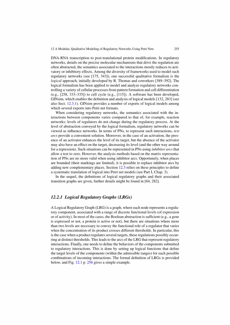
A Logical Regulatory Graph (LRG) is a graph, where each node represents a regula-tory component, associated with a range of discrete functional levels (of expressionor of activity). In most of the cases, the Boolean abstraction is sufficient (e.g., a geneis expressed or not, a protein is active or not), but there are situations where morethan two levels are necessary to convey the functional role of a regulator that varieswhen the concentration of its product crosses different thresholds. In particular, thisis the case when a product regulates several targets, these regulations possibly occur-ring at distinct thresholds. This leads to the arcs of the LRG that represent regulatoryinteractions. Finally, one needs to define the behaviors of the components submittedto regulatory interactions. This is done by setting up logical functions that definethe target levels of the components (within the admissible ranges) for each possiblecombinations of incoming interactions. The formal definition of LRGs is providedbelow, and Fig. 12.1 p. 256 gives a simple example.


Fig. 12.1 Example of an LRG. The regulatory graph is displayed in the higher level, with thenodes denoting components and the arcs denoting interactions (arcs with normal arrows denoteactivations, whereas arcs with blunt end denote repressions). The logical functions are then givenin the form of tables (one for each component), where each row corresponds to (a set of) state(s)with the corresponding function values (! denotes one value among all possible values, 1–2 de-notes value 1 or 2, etc.). For example, the table on the left defines the logical function KG0, whichonly depends on the levels of G1, the sole regulator of G0. The IDD representation of each logicalfunction is given in the lower level (see Sect. 12.2.2 for explanations). For instance, G3 has tworegulators (G0 and G1), its logical function KG3 specifies that, when both regulator levels arelower than 2, whatever the levels of the other components (which have indeed no effect on G3),the target level of G3 is 0 (first row of the table defining KG3). The IDD representing KG3 en-compasses the decision variables x0 and x1 (the levels of G3 regulators) and the case just describedis recovered by following the edges going out x0 and x1 labeled [0,1], which leads to a leaf labeled0 (for readability, this leaf has been duplicated)

Definition 12.1 A logical regulatory graph (LRG) is defined as a labeled directedmultigraph1 R = (G ,E ,K ) where,

• G = {g1, . . . , gn} is the set of nodes, representing regulatory components. Eachgi " G is associated to its maximum level Maxi (Maxi " N!), its current levelbeing represented by the variable xi (xi " {0, . . . ,Maxi}). We define x =def

(x1, . . . , xn) the current state, and S =def!

gi"G {0, . . . ,Maxi} the set of all pos-sible states.

1A multigraph is a graph with possibly several edges between a pair of nodes.


• K = (K1, . . . ,Kn) defines the logical functions attached to the nodes specifyingtheir behaviors: Kj is a multi-valued logical function that gives the target levelof gj , depending on the state of the system: Kj : S # {0, . . . ,Maxj }.

• E is the set of oriented edges (or arcs) representing regulatory interactions. Anarc (gi, gj ) specifies that gi regulates gj (when there is no possible confusion,i stands for gi ), that is, Kj varies with xi . A regulatory graph may contain self-loops (an arc (i, i) represents a self-regulation of gi ).

For each gj " G , Reg(j) denotes the set of its regulators: i " Reg(j) if andonly if (i, j) " E .

Several remarks follow from Definition 12.1.

Remark 12.1 It is clear that, to determine the target level of a component, onlythe levels of its regulators are required (other components have no effect). In otherwords, Kj can be defined on the restricted domain

!gi"Reg(j){0, . . . ,Maxi}. For

example, in Fig. 12.1, since G1 is the sole regulator of G0, we could restrict thedomain of KG0 to {0, . . . ,MaxG1} (indeed, in the table defining KG0, we can verifythat the values of G0, G2 and G3 do not matter).

Remark 12.2 If gi " Reg(j) and Maxi > 1 (gi regulates gj and is multi-valued), gi

may have different effects onto a component gj , depending on the current level of gi ,leading to the definition of a multi-arc between gi and gj . Such a situation typicallyhappens when a component has a dual regulatory role, for example, activation atlow and repression at high concentrations.

Here, to avoid the cumbersome notations resulting from such multi-arcs, we as-sume that all interactions are simple. However, it is straightforward to generalizeall the definitions introduced in this chapter to LRGs encompassing multi-arcs (see,e.g., [282]).

Remark 12.3 The biologists often associate signs to the regulatory interactions, dis-tinguishing between positive effect (activation or enhancing) and negative effect(repression or silencing). However, the actual effect of an interaction on its targetmay depend on the presence of cofactors; its sign may even change depending onthe context. In any case, the signs of interactions can be derived from the logicalfunctions K s. Moreover, a threshold ! associated to an interaction from gj to gi

with 1 $ ! $ Maxj indicates for which level of gj the interaction is active (i.e.,when xj % ! , (gj , gi) is active). This threshold can also be recovered from the func-tion Ki : ! is the value for which there exists x " S such that for x& defined asx&k =def xk,'k (= j and x&j =def xj + 1 = ! , we have Ki (x) (= Ki (x

&). For example,in Fig. 12.1 the interaction from G0 to G1 is associated with a threshold 1 and apositive sign; this is visible by comparing the first and third rows of the table defin-ing KG1 (also the second and the fourth rows), where, for fixed values of the othercomponents, changing G0 level from 0 to 1 leads to a change in the target value ofG1 from 0 to 1. Whereas the interaction from G0 to G3 is associated with a thresh-old 2 with a negative sign (determined by comparing second and third lines of KG3table).


Finally, it is worth noting that a set of logical functions Ki , i = {1, . . . , n},fully defines an LRG encompassing n regulatory components. In particular,for each i " {1, . . . , n}, its maximum level is given by the maximum valueof Ki .

12.2.2 Logical Functions Representation Based on DecisionDiagrams

In [282], logical functions were represented by means of Reduced Ordered Multi-valued Decision Diagrams (ROMDDs, referred to as MDDs in the following). Thisrepresentation, internally used in GINsim for efficiency purposes, facilitates the def-inition of algorithms for the analysis of logical models (e.g., see the stable state de-termination described in [282]). The use of MDDs also makes the definition of theP/T net representation of logical models easier and more concise than that proposedin for example, [65]. This representation, which is quite intuitive, is informally pre-sented below.

Binary Decision Diagrams (BDDs) are a convenient data structure to repre-sent Boolean functions [52]. A BDD is a rooted, directed, acyclic graph, en-compassing decision nodes (labeled by a Boolean variable) and two leaves (alsocalled terminal-nodes) labeled respectively, 0 (false) and 1 (true). Decision nodeshave two successors (or children): the left (resp. right) outgoing edge representsan assignment of the variable to 0 (resp. to 1). Most BDDs are ordered andreduced, meaning that variables appear in the same order along all the pathsfrom the root, and that all isomorphic (equal) subgraphs are merged and nodeshaving two isomorphic children are deleted (see Fig. 12.2 for an illustration).This structure has been naturally extended to handle discrete multi-valued func-tions, which are then represented by Multi-valued Decision Diagrams (MDDs),where the decision nodes have as many children as the number of their possi-ble values and the leaves (or terminal nodes) are labeled by the values of thefunction [179]. The ordering and reduction rules defined for binary decision di-agrams apply also to this multi-valued generalization (see [52] for further de-tails). A path from the root to a leaf represents a (possibly partial) assignment ofthe decision variables for which the function takes the value carried by the leaf(see Fig. 12.2).

In the MDD representation of the function Ki of a regulatory component gi , thedecision variables are the variables associated to the regulators of gi , and the leavestake their values in [0,Maxi], which denotes the integer interval {0, . . . ,Maxi}. Notethat the use of a MDD leads to a simplified expression of Ki , but the resultingdiagram and its complexity may vary depending on the ordering of the decisionvariables [179].

Finally, it is possible to consider a compact representation of the usual MDD bymerging consecutive edges leading to the same child as explained hereafter.

Given gi " G , for each decision variable xj that appears in the diagram of Ki ,there are Maxj + 1 outgoing edges, implicitly labeled with the corresponding value


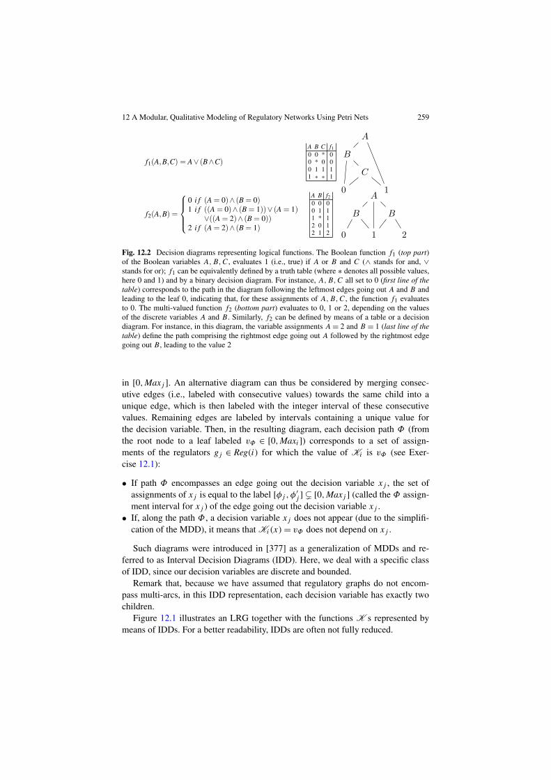
Fig. 12.2 Decision diagrams representing logical functions. The Boolean function f1 (top part)of the Boolean variables A,B,C, evaluates 1 (i.e., true) if A or B and C () stands for and, *stands for or); f1 can be equivalently defined by a truth table (where ! denotes all possible values,here 0 and 1) and by a binary decision diagram. For instance, A,B,C all set to 0 (first line of thetable) corresponds to the path in the diagram following the leftmost edges going out A and B andleading to the leaf 0, indicating that, for these assignments of A,B,C, the function f1 evaluatesto 0. The multi-valued function f2 (bottom part) evaluates to 0, 1 or 2, depending on the valuesof the discrete variables A and B . Similarly, f2 can be defined by means of a table or a decisiondiagram. For instance, in this diagram, the variable assignments A = 2 and B = 1 (last line of thetable) define the path comprising the rightmost edge going out A followed by the rightmost edgegoing out B , leading to the value 2

in [0,Maxj ]. An alternative diagram can thus be considered by merging consec-utive edges (i.e., labeled with consecutive values) towards the same child into aunique edge, which is then labeled with the integer interval of these consecutivevalues. Remaining edges are labeled by intervals containing a unique value forthe decision variable. Then, in the resulting diagram, each decision path " (fromthe root node to a leaf labeled v" " [0,Maxi]) corresponds to a set of assign-ments of the regulators gj " Reg(i) for which the value of Ki is v" (see Exer-cise 12.1):

• If path " encompasses an edge going out the decision variable xj , the set ofassignments of xj is equal to the label [#j ,#

&j ] ! [0,Maxj ] (called the " assign-

ment interval for xj ) of the edge going out the decision variable xj .• If, along the path " , a decision variable xj does not appear (due to the simplifi-

cation of the MDD), it means that Ki (x) = v" does not depend on xj .

Such diagrams were introduced in [377] as a generalization of MDDs and re-ferred to as Interval Decision Diagrams (IDD). Here, we deal with a specific classof IDD, since our decision variables are discrete and bounded.

Remark that, because we have assumed that regulatory graphs do not encom-pass multi-arcs, in this IDD representation, each decision variable has exactly twochildren.

Figure 12.1 illustrates an LRG together with the functions K s represented bymeans of IDDs. For a better readability, IDDs are often not fully reduced.


12.2.3 State Transition Graphs Associated to LRGs

The behavior of a logical regulatory graph is defined by the logical functions intro-duced in Definition 12.1. For any state of the system (i.e., a vector encompassingthe levels of all the regulatory components), these functions indicate the target levelof each component, that is the level to which it evolves. State Transition Graphs(STGs) constitute a classical and convenient way of representing the behavior ofsuch systems. In these directed graphs, nodes represent states, and arcs representtransitions between states that amount to update one component level (increasing ordecreasing it by one).

Definition 12.2 Given an LRG R = (G ,E ,K ), its full State Transition Graph(STG) is a directed graph (S ,T ) such that:

• the set of nodes is the set of states S as defined above,• T +S 2 defines the set of transitions (arcs) as follows. For all (x, y) "S 2:

(x, y) "T ,- .gi " G s.t.

"#

$

Ki (x) (= xi,

yi = $i (x) =def xi + sign(Ki (x)/ xi),

yj = xj 'j (= i.

Given an initial state x0, we further define the STG (S|x0 ,T|x0), which containsall states reachable from x0:

• x0 "S|x0 ,• 'x "S|x0 , 'y "S , (x, y) "T - y "S|x0 and (x, y) "T|x0 .

The updating function $i of a regulatory component gi , as defined above, speci-fies the update of xi , the level of gi ; depending on the current state x of the network,the value of $i (x) is either xi (no change, xi = Ki (x)), xi + 1 (increase by one,xi < Ki (x)) or xi / 1 (decrease by one, xi > Ki (x)).

In Fig. 12.3 the full STG of the LRG of Fig. 12.1 is displayed, together with twosub-graphs obtained for different initial states. Analyzing an STG, we can recoverimportant properties of an LRG, among which:

• Single point attractors or stable states (e.g., corresponding to stable expressionpatterns) are nodes of the STG with no successor; in other words, they are statesin which all component levels are equal to the target value indicated by the logicalfunctions.

• Complex attractors (e.g., corresponding to oscillatory behaviors) are terminalstrongly connected components encompassing more than one node, that is, setssuch that all states are reachable from each other along directed paths, and thereis no outgoing transition; in other words, the system is trapped in such a set onceit has reached one of its state (see Exercise 12.2).

• Reachability of given attractors from initial conditions corresponds to the exis-tence of path(s) in the STG.


Fig. 12.3 State transition graphs corresponding to the LRG of Fig. 12.1. On top, the full STG,encompassing all 36 states. Note that there are two stable states indicated as ellipse nodes:(xG0, xG1, xG2, xG3) = (2,2,1,0) and (0,0,0,0). Other transient states are denoted as rectan-gular nodes. The two graphs in the lower part of the figure correspond to sub-graphs of the fullSTG for the initial states (0,0,1,0) (on the left) and (1,2,1,0) (on the right). Note that, for theinitial state (1,2,1,0), one stable state is lost

12.3 P/T Petri Net Representation

The Definition 12.3 below explicitly defines a P/T net associated to an LRG, usingthe IDD representation of the functions Kis (as introduced in Sect. 12.2.1). Furtherdetails, basic properties and applications of this P/T net representation of LRGs areprovided in [65] for the Boolean case, and in [66, 68] for the multi-valued one.

Definition 12.3 Given an LRG R = (G ,M ax,E ,K ), we define the correspond-ing Multi-valued Regulatory Petri Net (MRPN) as follows:


• For each gi " G , two complementary places are defined, gi and %gi , satisfying, forall marking M :

M(gi) + M&%gi

'= Maxi . (12.1)

• For each gi " G , for each path " from the root to a leaf of the IDD represent-ing Ki , at most two transitions are defined, one accounting for the increasing shift(denoted t+i," ), the second accounting for the decreasing shift (denoted t/i," ) (thissimplifies when the leaf is associated with an extreme value, see below). Recallthat " defines assignment intervals of the levels of gj in Reg(i): xj " [#j ,#

&j ],

with #j ,#&j " [0,Maxj ] and #j $ #&j .

• Transitions t+i," and t/i," are connected to:– place gj , j " Reg(i), with a test arc weighted #j ,– place %gj , j " Reg(i), with a test arc weighted Maxj / #&j .Transition t+i," is further connected to:– place gi , with an outgoing arc (increasing the level of gi ),– place %gi , with an incoming arc weighted Maxi / v" + 1 (ensuring that the

current level of gi is less than the focal value v" ) and an outgoing arc weightedMaxi/v" (accounting for the decreasing by one of the current marking of thiscomplementary place).

Symmetrically, transition t/i," is further connected to:– place %gi , with an outgoing arc (decreasing the level of gi ),– place gi , with an incoming arc weighted v" + 1 (ensuring that the current

level of gi is greater than the focal value v" ) and an outgoing arc weighted v"(accounting for the decreasing by one of the current marking).

From the definition above, it follows that, for all gi " G and " a path in thedecision diagram associated to Ki , when v" = 0 or v" = Maxi (the value of theKi for this assignment of the regulators is extreme), only one transition is relevant.Indeed, if v" = 0, transition t+i," can be omitted as, by construction, there will neverbe Maxi + 1 tokens in place %gi . Similarly, if v" = Maxi , transition t/i," can beomitted as there will never be Maxi + 1 tokens in place gi . Moreover, for gj "Reg(i), when #j = #&j , from (12.1), it suffices to consider only one test arc (thattowards place gj for example).

Given an LRG R and an IDD representation of its logical functions, the Defini-tion 12.3 uniquely specifies a P/T net. It can be shown that, given an initial state x0,the STG (S|x0 ,T|x0) is isomorphic to the marking graph of the P/T net with theinitial marking defined as M0(gi) = x0

i and M0(%gi) = 1/ x0i , for all components gi

(see proof in [68]). Hence, properties of an LRG can be derived from the analysisof the marking graph of its P/T net representation.

The IDD representation of the logical function leads to more compact Petri netscompared to those obtained by using decision trees or truth table representations(as in [66]). Different orderings of the variables in the IDD may generate differentreductions. However, although the number of transitions may vary, it can be provedthat the resulting dynamics (the marking graphs) are identical [68].

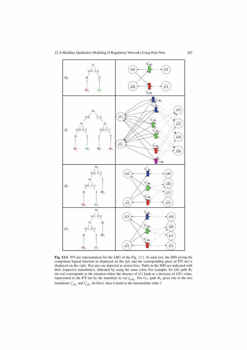
Figure 12.4 illustrates this P/T net representation for the LRG of the Fig. 12.1.


Fig. 12.4 P/T net representation for the LRG of the Fig. 12.1. In each row, the IDD giving thecomponent logical function in displayed on the left, and the corresponding piece of P/T net isdisplayed on the right. Test arcs are depicted as dotted lines. Paths in the IDD are indicated withtheir respective transition(s), indicated by using the same color. For example, for G0, path "1(in red) corresponds to the situation where the absence of G1 leads to a decrease of G0’s value,represented in the P/T net by the transition in red t/0,"1

. For G1, path "3 gives rise to the twotransitions t/1,"3

and t+1,"3(in blue), since it leads to the intermediate value 1


12.3.1 Tools Support

GINsim is a software dedicated to the definition and analyze of regulatory networkslogical models [132, 283]. With the representation presented in Sect. 12.3 we canalso employ PN tools to analyze (larger) LRGs. GINsim has been equipped withexport functionalities generating files in the INA [166] format, PNML (Petri netmarkup language) [306] and APNN (Abstract Petri Net Notation) [29].

In the case of the analysis of the segment-polarity system as defined in [335], thereachability analysis of the expected patterns was performed using INA. We havealso assessed the high complexity of the STG of this model, using tools such as themodel-checking tool DSSZ-MC [101] and Tina [393].

12.3.2 Related Works

Related works include the representation of logical regulatory networks by meansof high-level Petri nets. In [66] a high-level PN representation of LRGs is defined,encompassing one place and one transition for each regulatory component. The evenmore compact representation defined in [81] enables the verification of the modelcoherence under various hypotheses (accounting for observed biological behaviorssuch as homeostasis, multistationarity, or even more specific temporal properties).

Based on similar principles as exposed in this section, Steggles et al. have defineda Petri net representation of Boolean regulatory graphs [374]. However, to accountfor Boolean networks as introduced by Kauffman [185] which are synchronouslyupdated (meaning that all components are updated at once), a two-phase method isdefined to ensure the synchronization of the updates. The first phase identifies allcomponents that are called to change their values, the second phase performs thisupdate synchronously.

Finally, the PN representation of regulatory networks as presented here, enablesthe delineation of integrated models of regulated metabolic pathways, considering alogical model of the regulatory level (a PN representation) linked to a classical PNmodel of the metabolic part. In [362], this approach is illustrated with a qualitativemodeling of the biosynthesis of tryptophan (Trp) in E. coli.

12.4 Modules, Their Composition and High-Level Petri NetRepresentation

The framework presented in this section deals with collections of spatially dis-tributed abstract modules (nonnested) which may be cells, compartments in cellsor any subsystems that one wants to model separately. Each such module is definedby a regulatory network with identified inputs. The regulation functions take intoaccount spatial configuration between modules.


In a first step, we introduce Logical Regulatory Modules (LRMs) as LRGsequipped with external input nodes and arcs. Then, we define how such modulescan be spatially located and interconnected in order to form a Collection of in-terconnected Logical Regulatory Modules (CLRMs). Finally, given a collection oflogical regulatory modules, we define its high-level Petri net representation.

12.4.1 Interconnecting Logical Regulatory Modules

In what follows, a Logical Regulatory Module is defined as a uniquely identifiedlogical regulatory network associated with a set of input components that regulateinternal ones. Notice that no output nodes are defined because any internal com-ponent may generate an external signal towards other modules; moreover, inputcomponents are not effective regulatory components in that they do not introduceany intermediary step in the signaling. These inputs are meant to combine (or inte-grate) external signals from other modules. Functions % in Definition 12.4 performsuch combinations by calculating the levels of the integrated signals, depending onthe levels of the corresponding individual incoming signals and on their attributedweights. These weights, defined as real numbers on the interval [0;1], encode neigh-boring relations, which in turn are defined when interconnecting the modules (seeDefinition 12.5). Hence, at this stage, in order to define a logical regulatory mod-ule, one has to specify the components that are likely to signal the module, andhow input signals are combined through the functions % . If needed, both constraintscould be relaxed. In particular, postponing the specification of functions % to theactual connection of modules would be a straightforward extension of the currentframework.

Definition 12.4 Given & a domain of regulatory components, a Logical RegulatoryModule (LRM) M is a tuple (G ,E ,' ,%,K ), where

• G + & is the set of internal components;• E + G 0 G is the set of internal interactions between internal components;• ' + & is the set of input components;• % = {%v,g | (v, g) "E + ' 0 G } is a set of integration functions,

%v,g :&{0, . . . ,Maxv}0] 0;1]

'! # {0, . . . ,Maxg}computing the combined level for all inputs v regulating g. Their arguments arepairs (xv, dv) where each xv is the level of v in one neighbor, weighted by dv > 0;

• K is a set of logical functions defined on G giving, for each component g " G ,its target level in {0, . . . ,Maxg}, depending on the levels of its regulators. For aninternal regulator r (r " G ) the level used to evaluate Kg is xr as usual, while foran input regulator v (v " ' ), the level used to evaluate Kg is the current valueof %v,g . We denote by args(Kg) the set of arguments of Kg .


Fig. 12.5 A “toy” LRM M with: G =def {A,B,C}, E =def {(A,C), (C,B), (B,A)}, ' =def {B},with, e.g., %B,C =def (yj , dj )j%0 1# round(max(yj · dj )), and K being defined on the right partof the figure. The input node B is depicted as a gray node. We have args(KC) = {A,%B,C}

Figure 12.5 provides a simple example of an LRM. If %v,g " args(Kg), then v isan input regulator of g; in the pictures, this is denoted by an arc toward the node g.

An LRM can be viewed as an encapsulated regulatory network with input nodesbehaving as integrators of external signals of the corresponding components fromother modules. For example, for the LRM depicted in Fig. 12.5, the level of externalsignal corresponding to B will be calculated as a weighted maximum over all thelevels of B in neighboring modules (i.e., having a nonzero weight). Hence, thislevel can be evaluated only when the module is connected to other modules (seeDefinition 12.5). Nevertheless, at this stage, it is possible to recover a fully definedLRG, by setting the integration functions and specifying the behaviors of the inputcomponents (for example, as having constant levels).

Notice that, like in the Fig. 12.5, it is not required that G 2 ' = 3. For example,we may have g " G 2' when the regulatory component g has both autocrine (actingon the same cell) and paracrine effects (acting on neighboring cells). Then g " Gaccounts for the autocrine effect and g " ' accounts for the paracrine effect (as in thecase of Wingless in the Drosophila segment polarity module depicted in Sect. 12.5).

We now proceed with collections of LRMs, which contain all the informationneeded to interconnect LRMs through their input nodes. It simply consists in defin-ing a set of LRMs and a topological relation between these LRMs that establishesthe actual connections between modules and allows the evaluation of the levels ofinput components.

Definition 12.5 A Collection of interconnected Logical Regulatory Module(or CLRM) is defined as a triplet (I,M,T), where:

• I4N is a finite set of integers (module identifiers);• M = {(m,M ) | m " I} is a set of LRMs, each being associates to an identifier

in I;• T : I 0 I \ {(m,m) | m " I}#[ 0;1], is a topological (or neighboring) relation

between modules in M; the values of T can be interpreted as weights associatedto external signals.

In a CLRM, one can define several copies of the same LRM (these copies aredistinguished by their identifiers). This is the case in Fig. 12.6 that shows a CLRMencompassing three times the LRM of Fig. 12.5. Notice the dashed arcs that repre-sent how each LRM signals its neighbors according to the topological relation.


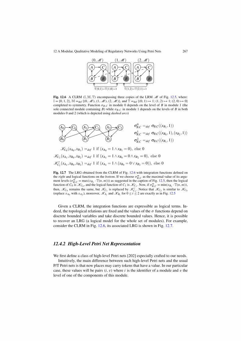
Fig. 12.6 A CLRM (I,M,T) encompassing three copies of the LRM M of Fig. 12.5, where:I = {0,1,2}, M =def {(0,M ), (1,M ), (2,M )}, and T =def {(0,1) 1# 1; (1,2) 1# 1; (2,0) 1# 0}completed to symmetry. Function %B,C in module 0 depends on the level of B in module 1 (thesole connected module containing B) while %B,C in module 1 depends on the levels of B in bothmodules 0 and 2 (which is depicted using dashed arcs)

Fig. 12.7 The LRG obtained from the CLRM of Fig. 12.6 with integration functions defined onthe right and logical functions on the bottom. If we choose %m

B,C as the maximal value of its argu-ment levels (%m

B,C = max(xBn · T(n,m))) as suggested in the caption of Fig. 12.5, then the logicalfunction of C0 is KC0 , and the logical function of C1 is KC1 . Now, if %m

B,C = min(xBn · T(n,m)),then, KC0 remains the same, but KC1 is replaced by K &

C1. Notice that KC2 is similar to KC0

(replace xA0 with xA2 ), moreover, KAi and KBi for 0$ i $ 2 are exactly as in Fig. 12.5

Given a CLRM, the integration functions are expressible as logical terms. In-deed, the topological relations are fixed and the values of the % functions depend ondiscrete bounded variables and take discrete bounded values. Hence, it is possibleto recover an LRG (a logical model for the whole set of modules). For example,consider the CLRM in Fig. 12.6, its associated LRG is shown in Fig. 12.7.

12.4.2 High-Level Petri Net Representation

We first define a class of high-level Petri nets [202] especially crafted to our needs.Intuitively, the main difference between such high-level Petri nets and the usual

P/T Petri nets is that now places may carry tokens that have a value. In our particularcase, these values will be pairs (i, v) where i is the identifier of a module and v thelevel of one of the components of this module.


Fig. 12.8 The marking depicted on the left represents the fact that, for module 0, xA = 1 andxB = 0, and, for module 1, xA = 0 = xB . For this marking, transition tA is enabled for the binding( = (µ# 0, xAµ # 1, xBµ # 0). Suppose $A(1) = 0 ($A being the updating function), the firingof tA leads to the marking depicted on the right of the picture. This corresponds to a state changein the biological system

In order to consume and produce tokens when a transition fires, arcs are labeledwith expressions involving variables; an empty label denotes the absence of arc.At fire time, it is necessary to bind (i.e., to map) each such variable to a concretevalue so that the annotation on each arc can be evaluated to a collection of tokens.A binding ( is a function that maps variables to values. We denote ((expr) theevaluation of an expression expr under the binding ( .

More precisely, a high-level Petri net is a tuple (S,T ,)), where:

• S is the set of places, each place is allowed to carry structured tokens from N0N.• T , disjoint from S, is the set of transitions.• ) : (S 0 T )5 (T 0 S) defines the labeling of the arcs by expressions.

In general, a marking M of a high-level Petri net is a mapping associating to eachplace s " S a multiset over N0N representing the tokens held by s at M . However,in our case, markings are always sets (in all evolutions, no token may be duplicatedin the same place). So, we assume that arc labels always evaluate to sets of tokens.

A transition t may fire at a marking M with binding ( if there are enough tokensin the input places of t : for all s " S, (()(s, t))+M(s). If so, t may fire and producea new marking M &, where M & is M in which consumed tokens are removed andproduced tokens are added, that is, for all s " S: M &(s) =def (M(s) \ (()(s, t))) 5(()(t, s)), see Fig. 12.8.

Remark 12.4 For the sake of simplicity, Definition 12.6 below is valid only if mod-ules do not overlap, that is, for (m,M ) and (n,N ) two LRMs in M, (M (= N )-(G m 2 G n = 3). This means that the set of all regulatory components is partitionedand we can focus on the evolution of each species in the context of the set of (iden-tical) modules it belongs to.

Let Kg be the logical function of g. As previously, we define the updating func-tion $g(xgm) =def xgm + sign(Kg(· · ·)/ xgm) where Kg is computed with the ap-propriate arguments (including integration functions calls) as defined above.

Each internal regulatory component g " G is modeled by a high-level Petri netplace sg that stores the numeric value of the corresponding level for each module m.In order to model several modules (each having a unique identifier), each place holds


tokens of the form (m,xg), where m " I and xg is the level of g in module m. Theevolution of each regulatory component g " G is implemented by a unique transitiontg that consumes the value of g in m (token (m,xg) from place sg), reads the valuesof the regulators of g, and produces the new level $g(xgm) of g in m. Thus, transitiontg has all the necessary arcs to the places modeling g and its regulators.

Definition 12.6 Let (I,M,T) be a CLRM. We denote G =def(

m"I G m the set ofcomponents involved in the CLRM. The high-level Petri net associated to (I,M,T)

is (S,T ,)), defined as:

• S =def {sg | g " G }• T =def {tg | g " G }• For each g " G , let m denotes the LRM such that g " G m, the arcs attached to

each tg " T are as follows:– First, a pair of arcs allows to read and update the current level of g for module

M , whose identifier m is captured by a net variable µ:– If %g,g /" args(Kg), there is one arc (sg, tg) labeled by {(µ,xgµ)} and one

arc (tg, sg) labeled by {(µ, $g(xgµ))}.– Otherwise, there is one arc (sg, tg) labeled by {(µ,xgµ)} 5{ (*, xg* ) | '* :

T(µ,*) > 0} and one arc (tg, sg) labeled by {(µ, $g(xgµ))}5{ (*, xg* ) | '* :T(µ,*) > 0}; it means that the levels of g in all modules * in the neighboringof m are read and only the level of g in m is updated.

– Then, for each g& " G m \ {g}, a test arc (sg& , tg) is added to bind the parametersof the logical and integration functions, with net variable µ capturing as abovethe identity of module m:– If (g&, g) " E m and %g&,g /" args(Kg) (g& is only an internal regulatory), this

arc is labeled by {(µ,xg&µ)}.– If (g&, g) " E m and %g&,g " args(Kg) (g& is both an internal and external

regulator), this arc is labeled by {(µ,xg&µ)}5{ (*, xg&*) | '* : T(µ,*) > 0}.– If (g&, g) /" E m and %g&,g " args(Kg) (g& is only an external regulator), this

arc is labeled by {(*, xg&*) | '* : T(µ,*) > 0}.

For the collection in Fig. 12.7, we obtain the Petri net depicted in Fig. 12.9.

12.4.3 Implementation

A prototype of the construction presented above has been implemented on the top ofSNAKES toolkit [307]. SNAKES is a full featured Petri net library intended for quickprototyping; it uses Python programming language [313] to express the various Petrinet annotations. Using this implementation:

• LRMs can be fully specified as Python classes.• Arbitrary integration functions can be user-defined, some are predefined.• CLRMs can be defined by composing LRM instances with arbitrary topologies.


Fig. 12.9 The high-level Petri net representation of the CLRM of Fig. 12.7. A possible initialmarking may be M0 as given below the Petri net

• CLRMs topology can be drawn with automatic layout.• All possible stable states of a CLRM can be computed.• Reachable states from an initial one can also be computed, with extraction of the

reachable stable states.

12.5 Modeling Interconnected LRMs Using High-Level PetriNets

In this section, we illustrate the modeling of interconnected logical regulatory mod-ules by means of high-level Petri nets. In a first step, we analyze nine cases of col-lections of several copies of our toy LRM (as defined in Fig. 12.5). We show howvariations of the topological or the integration functions can affect the behaviors ofthe whole model. Then we discuss the application of our framework to the model-ing of the segment-polarity module involved in the segmentation of the Drosophilaembryo.

In both cases, the considered collection of modules is composed of copies of thesame LRM. This, indeed, will mostly be the case when modeling patches of identicalcells, but one should be aware that the proposed framework does not impose such arestriction.

12.5.1 Interconnecting Occurrences of the Toy LRM

Let consider the toy LRM M as defined in Fig. 12.5. In this section, we analyze thebehaviors of a series of collections encompassing a number of occurrences of M .


Fig. 12.10 The various topologies considered for 2-width tapes. On the left, the graphical viewshowing the organization of the connections. Definitions on the right side rely on the assump-tion that modules on the top line of the tape are numbered with consecutive even numbers, whilemodules on the bottom line are numbered (following the same direction) with consecutive oddnumbers. All topologies considered here are symmetrical, the subscript k indicates the maximalnumber of neighbors in the topology Tk in an extended grid (e.g., with the topological relation T4,any module would have at most 4 neighbors)

All the considered collections are based on a tape of modules of width 2, with var-ious lengths and topologies as depicted in Fig. 12.10. Each topological relation Tk

is called in such a way because modules may have neighbors in k directions. More-over, we denote Toy(n, k) the CLRM containing 2 · n copies of M arranged usingTk on a tape, as illustrated in Fig. 12.10.

All stable states of systems Toy(n, k) are such that the levels of the componentsin each module are equal (components A,B and C all equal to 0 or all to 1). So, todepict such a module stable state, we shall print a black and white grid, where black(resp. white) positions correspond to modules whose components are all 1 (resp.all 0), these positions respecting the topological relations of the modules. To sim-plify the presentation, we have also considered initial states that can be representedin this way.

Figure 12.11 shows the stable states that can be reached from chosen initial states.We can observe variations in the number of reachable states (which correspond tothe size of the marking graph) and of reachable stable states; moreover, the stablestates themselves are different.

All these examples have been obtained using the integration function %B,C de-fined as (yi, di)1$i$k # round(max(yi · di | 1$ i $ k)) (i.e., %B,C evaluates to themaximal value of B in neighboring modules; that is to say %B,C is 1 provided thatat least one neighboring module encompasses a component B which level is 1). Wemay consider instead a function that returns 1 if at least two components B in theneighboring modules are equal to 1, and return 0 otherwise. In this case, the be-haviors of the collections might be rather different; in particular, the initial statesconsidered for Toy(3,4) and Toy(4,4) (Fig. 12.11, fourth and seventh rows) turn tobe stable.


Fig. 12.11 Impact of the topological relation on the behaviors of the collections Toy(n, k), definedon the LRM of Fig. 12.5. In each row, a different combination of values of n and k (i.e., differentnumber of modules and topological relation) is considered: on the left, the initial collection state isdepicted, that is, the initial state of each of its modules (black if internal A, B , C are all 1, whiteif they are all 0), and on the right, the total number of reachable states is given and the reachablestable states are depicted. The top-left module of each state is decorated with links showing thedirections of its potential neighbors, for example, in T(3,8), a module has possibly 8 neighbors(see Fig. 12.10). This series of experiments shows that, for the same initial condition, a collectionof interconnected modules can behave differently, depending on the signaling capacities (expressedhere in terms of topological relations). For example, in the first collection T(2,4), the modules arenot able to signal along the diagonal, contrary to the collection T(2,8). In the first, the initial patternis stable, whereas it is not in T(2,8), which instead will stabilize in one of three other patterns.The integration function %B,C considered here takes the maximal value of B over the neighboringmodules


Fig. 12.12 Schematic illustration of the patterns of expression along the antero-posterior axis, inthe last step of the genetic hierarchy controlling the Drosophila segmentation: (top) the antero-pos-terior axis; (middle) initial activation of En (Engrailed) and Wg (Wingless) by the pair-rule signalsin stripes of cells (here, we considered that six cells are sufficient to represent the different regionsof a parasegment, which includes the posterior part of a segment and the anterior part of the nextsegment); (bottom) the consolidation and refinement of the parasegmental border by the action ofthe polarity genes, which requires cell-cell communication

12.5.2 The Drosophila Segment-Polarity Module

Early development of the fruit fly embryo is an ideal, very well-studied system fordevelopmental biologists (see [128, 417] for good introductions to this topic). Theembryo is organized into a series of segments along its antero-posterior axis (fromthe head to the tail). These segments will give rise to adult structures (legs, halteres,wings, etc.). This organization is initiated by maternal morphogens, which controlfew dozens of genes involved in the initial segmentation. These genes have beensplit into several classes. The first classes, called gap, pair-rule and segment-polaritymodules, constitute a temporal hierarchical genetic system. Segment-polarity genesare under the control of the pair-rule genes. Their patterns of expression define theanterior and posterior parts of the segments and they are responsible for the stabi-lization of the borders between embryonic segments (see Fig. 12.12). The segment-polarity module involves about twenty genes, cross-regulations and intercellular sig-nalings. It has been the subject of a wealth of theoretical modeling studies, in bothcontinuous (e.g., [87, 168]) and logical (e.g., [5, 69, 335]) frameworks.

In [335], a logical model is defined and analyzed, based on an intracellular in-teraction network of a dozen of components, submitted to two external inputs (theWingless (Wg) and Hedgehog (Hh) signalings). Six copies of this module have beeninterconnected in a stripe to allow the representation of the different gene expressiondomains flanking the parasegmental borders (parasegments correspond to portions


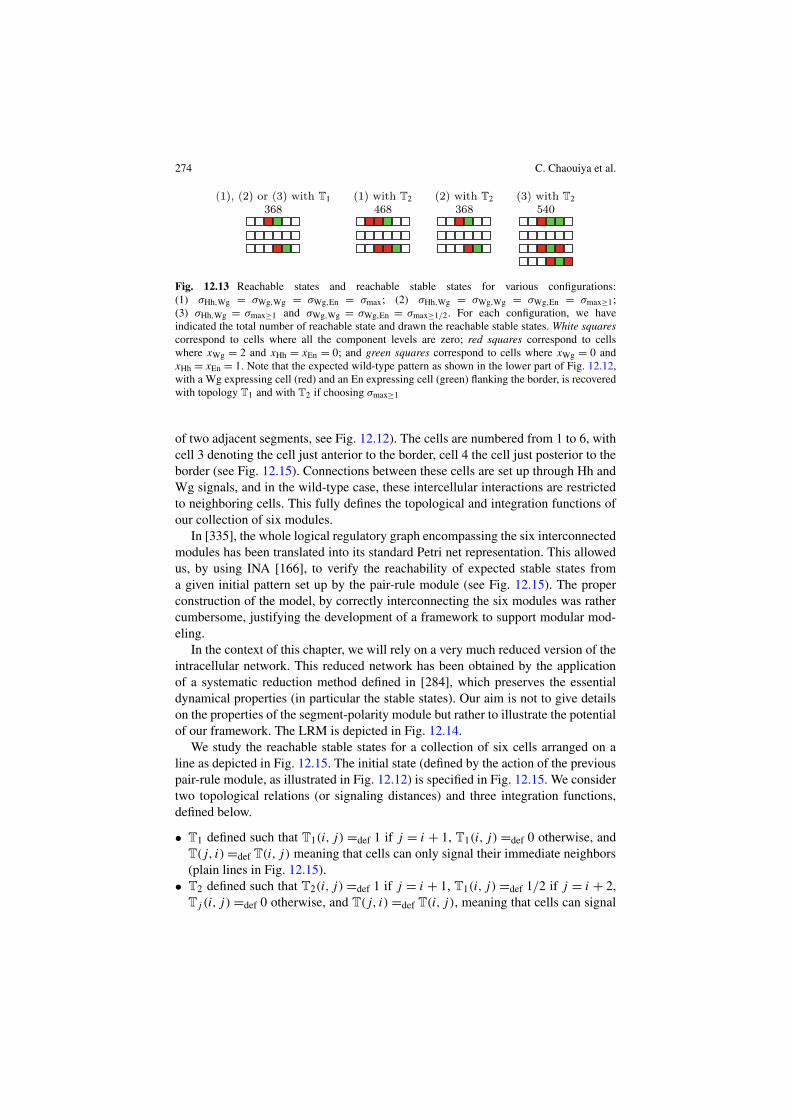
Fig. 12.13 Reachable states and reachable stable states for various configurations:(1) %Hh,Wg = %Wg,Wg = %Wg,En = %max; (2) %Hh,Wg = %Wg,Wg = %Wg,En = %max%1;(3) %Hh,Wg = %max%1 and %Wg,Wg = %Wg,En = %max%1/2. For each configuration, we haveindicated the total number of reachable state and drawn the reachable stable states. White squarescorrespond to cells where all the component levels are zero; red squares correspond to cellswhere xWg = 2 and xHh = xEn = 0; and green squares correspond to cells where xWg = 0 andxHh = xEn = 1. Note that the expected wild-type pattern as shown in the lower part of Fig. 12.12,with a Wg expressing cell (red) and an En expressing cell (green) flanking the border, is recoveredwith topology T1 and with T2 if choosing %max%1

of two adjacent segments, see Fig. 12.12). The cells are numbered from 1 to 6, withcell 3 denoting the cell just anterior to the border, cell 4 the cell just posterior to theborder (see Fig. 12.15). Connections between these cells are set up through Hh andWg signals, and in the wild-type case, these intercellular interactions are restrictedto neighboring cells. This fully defines the topological and integration functions ofour collection of six modules.

In [335], the whole logical regulatory graph encompassing the six interconnectedmodules has been translated into its standard Petri net representation. This allowedus, by using INA [166], to verify the reachability of expected stable states froma given initial pattern set up by the pair-rule module (see Fig. 12.15). The properconstruction of the model, by correctly interconnecting the six modules was rathercumbersome, justifying the development of a framework to support modular mod-eling.

In the context of this chapter, we will rely on a very much reduced version of theintracellular network. This reduced network has been obtained by the applicationof a systematic reduction method defined in [284], which preserves the essentialdynamical properties (in particular the stable states). Our aim is not to give detailson the properties of the segment-polarity module but rather to illustrate the potentialof our framework. The LRM is depicted in Fig. 12.14.

We study the reachable stable states for a collection of six cells arranged on aline as depicted in Fig. 12.15. The initial state (defined by the action of the previouspair-rule module, as illustrated in Fig. 12.12) is specified in Fig. 12.15. We considertwo topological relations (or signaling distances) and three integration functions,defined below.

• T1 defined such that T1(i, j) =def 1 if j = i + 1, T1(i, j) =def 0 otherwise, andT(j, i) =def T(i, j) meaning that cells can only signal their immediate neighbors(plain lines in Fig. 12.15).

• T2 defined such that T2(i, j) =def 1 if j = i + 1, T1(i, j) =def 1/2 if j = i + 2,Tj (i, j) =def 0 otherwise, and T(j, i) =def T(i, j), meaning that cells can signal


Fig. 12.14 A reduced version of the segment-polarity logical regulatory module (obtained fromthe model of 12 components of Sánchez [335], applying the reduction method presented in [284]).In this network, we kept the components exerting external signals (Wg and Hh) and the read-outgenes of the action of this regulatory network (En and Wg). The external signals (coming fromneighboring cells) are denoted by gray nodes. Rectangular nodes denote multi-valued components(Wg) and ellipse nodes denote Boolean components. The logical functions of the three internalcomponents are given as logical rules

Fig. 12.15 A stripe of six cells with three cells accounting for the posterior region of a paraseg-ment (cells 1, 2, and 3) and three cells accounting for the anterior region of the next paraseg-ment (cells 4, 5, and 6), the parasegmental border being established between cells 3 and 4. Ineach cell, the initial levels of the components are indicated; each cellular state is given as a triplexWg, xEn, xHh. Plain lines denote where T1 and T2 are equal to 1 and dotted lines denote whereT2 is equal to 1/2 (in other words, these lines denote the signaling capacities between the cells)

their immediate neighbors (plain lines), but also their second neighbors, with alower weight (dotted lines in Fig. 12.15).

The integration functions we consider are:

• Maximum weighted level:

%max =def (vi, di)1$i$k # round&max(vi · di | 1$ i $ k)

'.

• Maximum level of direct neighbors:

%max%1 =def (vi, di)1$i$k #max(vi | 1$ i $ k, di = 1).


• Maximum level for neighbors with weight at least 1/2:

%max%1/2 =def (vi, di)1$i$k #max(vi | 1$ i $ k, di % 1/2).

For example, let consider the initial state depicted in Fig. 12.15, topology T2and %Wg,Wg, which integrates the Wg signal acting on Wg. If %Wg,Wg = %max, thevalue of the integrated signal is the maximal weighted level of Wg in neighboringmodules (including second neighbors), hence for the module 4, this value is 1: Wgis 0 in both direct neighbors and in the second neighbor (module 2), Wg is 2 witha weight equal to 1/2. If %Wg,Wg = %max%1, the value of the integrated signal is themaximal level of Wg in direct neighbors (weight greater than or equal to 1), henceis the case of module 4 it evaluates to 0. Finally, if %Wg,Wg = %max%1/2, the valueof the integrated signal is the maximal level of Wg in neighboring cells (direct ornot, that is, weight greater than or equal to 1/2 ), hence in the case of module 4, itevaluates to 2.

Figure 12.13 shows the results for various combinations of these parameters.When T1 is used, all neighbor signals have a weight 1, so we have %max = %max%1 =%max%2.

In [335], the model considered for the six cell stripe was based on the assumptionof short range Wg and Hh signals. Hence, to analyze the case of nkd loss-of-function(naked cuticle is one of the segment-polarity genes), it was necessary to considera rewired network, accounting for the increased diffusion of Wg. In the frameworkpresented here, such a change would only consist in modifying the topological func-tion.

12.6 Conclusions

In this chapter, we have presented a modeling framework combining the logicalformalism with Petri nets (PNs). The standard Petri net representation of logicalregulatory graphs, although not very legible, enables the use of existing PN analysistools such as INA. In this respect, GINsim provides export facilities to generate filesin the format expected by PN tools (e.g., INA [166]). Hence, a first advantage ofthe PN representation of logical regulatory graphs is the possibility to analyze themusing existing PN tools.

A challenging problem arises when considering regulated metabolic networks.PNs open the way to a qualitative integrated modeling of regulated metabolic path-ways as proposed in [362], properly connecting PN models of the biochemical path-way and the regulatory control (this being modeled as a logical regulatory graphexpressed in terms of a PN).

Developmental processes relate to cell differentiation and pattern formation. Inparticular, in this chapter, we have delineated a framework that allows the modelingof patches of communicating cells. To illustrate the potential of this framework, wehave considered the segment-polarity module involved in the segmentation of theDrosophila embryo. In such processes, one has to consider connections of several(intra)cellular regulatory networks. We propose to define these individual regulatory


networks as logical regulatory modules (LRMs), identifying input signals they canreceive from the outside. Then, a collection of such modules (a CLRM) can bedefined, by setting up the number and type of LRMs, as well as the rules governingtheir interconnections. From such a CLRM, a large logical regulatory network canbe recovered. This procedure could be easily implemented in GINsim.

More importantly, we have defined a compact and legible high-level Petri net(HLPN) representation of a CLRM. Implementation of this construction has beenprovided. HLPNs provide a flexible framework, which allows to easily model dif-ferent configurations of a patch of cells as well as topological relations (e.g., therange of a signal).

It is worth noting here, that the proposed framework allows the considerationof other situations than communicating cells within a patch. For example, in largeregulatory networks, modularity arises from physical delimitation or cellular com-partments (e.g., nucleus, cytoplasm) or from functional role. Recently, a modularlogical modeling of the budding yeast cell cycle has been delineated in [116]. In thiscase, modules corresponding to regulatory networks with distinct functional rolesin the cell cycle control, have common components. Hence, while composing thesemodules, one has to properly set up the logical rules of these common components.Based on the methodology proposed in [116], the framework presented in this chap-ter might be extended to handle overlapping modules.

Although modularity is now recognized as an important feature for large bio-logical networks, little formal work and tool development support combination orcomposition of regulatory networks (see [357] and references therein). In [357], theauthors address this question and distinguish between fusion, composition, aggre-gation and flattening as distinct processes for building larger models from smallerones. The HLPN framework presented in Sect. 12.4 can be viewed as a model ag-gregation, in that it is a reversible process (the modules are conserved). In termsof modeling tools, it is worth noting that ProMoT, a tool that eases the definitionand edition of modular models, supports the logical formalism [265]. It is based onprinciples that are quite similar to those presented in Sect. 12.4.

The main motivation to develop the framework proposed here is to study howexisting cellular processes are controlled. However, it could be useful in the field ofsynthetic biology that aims at designing novel artificial biological systems (see [100]and references therein). Indeed, synthetic biology relies on the concept of modular-ity, by conceiving building blocks and combining them [2]. So far, synthetic biologymainly designed intracellular gene networks, but synthetic multicellular systems in-volving cell-cell communication emerged in recent years (see, e.g., [28]).

The complexity of regulatory networks dealt by modelers calls for the develop-ment of original and efficient computational means. Here, we have defined a frame-work that greatly facilitates the definition of models encompassing interconnectedregulatory modules. However, we still need to make progresses to analyze such largemodels. Combining the logical and PN formalisms, as well as taking advantage ofthe modular structure of the models should allow the development of more efficienttools.


12.7 Problems

12.1 Give the MDD representation of the function f2 given in Fig. 12.2 consideringthe variables A and B in the reverse order (i.e., first B , then A). Transform theobtained MDD into an IDD (labeling the edges with integer intervals, and mergingthem when possible as explain in Sect. 12.2.2).

12.2 Consider the genetic regulatory network called repressilator as defined byElowitz and Leibler [109], which consists of three genes (denoted here A, B and C),connected in a negative circuit (each component represses its successor in the cir-cuit, and is repressed by its predecessor).

Assuming Boolean levels for A, B and C, all interaction thresholds are equal to 1,and the components share the same logical rule: K (0) = 1 and K (1) = 0, thatis, if the repressor is at level 0 (absent), the regulated component target level is 1(present), and the other way around. Draw the full STG of this model and verifythat it encompasses a unique complex attractor, reachable from any initial state.

12.3 Consider an LRG encompassing a component C regulated by A and B , bothpositively auto-regulated, with MaxA = MaxB = 1 and MaxC = 2. The logical func-tions KA, KB and KC are given by their MDD representations below (note that KA

and KB are the identity function). Give the logical expressions defining these threefunctions (using the connectors ) and * as in Fig. 12.2). Give the P/T representa-tion of this LRG (verify that the autoregulations define transitions that are uselesssince they are never enabled, see [68]).

12.4 Find another enabling binding for the high-level Petri net depicted in Fig. 12.8.Which module is involved by this binding and what are the corresponding levels xA

and xB? Assume that $A(xA) = 1 and fire the transition accordingly.

12.5 Construct the high-level Petri net representation of the CLRM depicted inFig. 12.15, including the initial marking. Indications:

1. Start with determining the arguments of each regulatory function, separating in-ternal and external regulators.

2. Draw each Petri net transition separately, together with the places for the neededregulatory components.


3. Merge these Petri net parts by collapsing the places that implement the sameregulators.

4. Add the initial marking, corresponding to the expression levels indicatedin Fig. 12.15.

Acknowledgements We thank G. Batt, A. Naldi, E. Remy, S. Soliman, D. Thieffry for fruitfuldiscussions. This work was supported by the French Research Agency (project ANR-08-SYSC-003).

chapter 12 a modular, qualitative modeling of regulatory...

Documents