chapter 12: firms in perfectly competitive...
TRANSCRIPT

1
1
Economics6th edition
Chapter 12Firms in Perfectly
Competitive Markets
Copyright © 2017 Pearson Education, Inc. All Rights Reserved
Copyright © 2017 Pearson Education, Inc. All Rights Reserved
2
Chapter Outline
12.1 Perfectly Competitive Markets
12.2 How a Firm Maximizes Profit in a Perfectly Competitive
Market
12.3 Illustrating Profit or Loss on the Cost Curve Graph
12.4 Deciding Whether to Produce or to Shut Down in the Short
Run
12.5 “If Everyone Can Do It, You Can’t Make Money at It”: The
Entry and Exit of Firms in the Long Run
12.6 Perfect Competition and Efficiency
Copyright © 2017 Pearson Education, Inc. All Rights Reserved
3
Market Structures
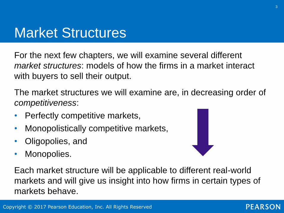
For the next few chapters, we will examine several different
market structures: models of how the firms in a market interact
with buyers to sell their output.
The market structures we will examine are, in decreasing order of
competitiveness:
• Perfectly competitive markets,
• Monopolistically competitive markets,
• Oligopolies, and
• Monopolies.
Each market structure will be applicable to different real-world
markets and will give us insight into how firms in certain types of
markets behave.
Copyright © 2017 Pearson Education, Inc. All Rights Reserved
4
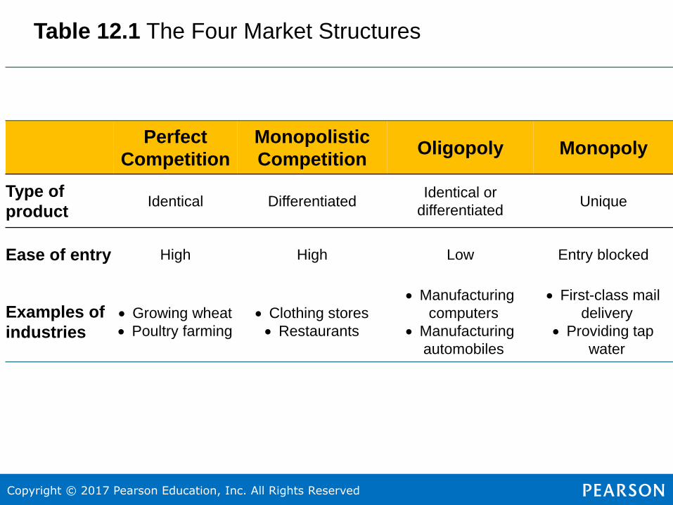
Table 12.1 The Four Market Structures
Perfect
Competition
Monopolistic
CompetitionOligopoly Monopoly
Type of
productIdentical Differentiated
Identical or
differentiatedUnique
Ease of entry High High Low Entry blocked
Examples of
industries
Growing wheat
Poultry farming
Clothing stores
Restaurants
Manufacturing
computers
Manufacturing
automobiles
First-class mail
delivery
Providing tap
water
Copyright © 2017 Pearson Education, Inc. All Rights Reserved
55
12.1 Perfectly Competitive Markets
Explain what a perfectly competitive market is and why a perfect competitor faces a
horizontal demand curve.
Key conditions for a perfectly competitive market:
1. There are many buyers and sellers,
2. All firms sell identical products, and
3. There are no barriers to new firms entering the market.
The first and second conditions imply that perfectly competitive
firms are price takers: they are unable to affect the market price.
This is because they are tiny relative to the market and sell exactly
the same product as everyone else.
Perfectly competitive markets are relatively rare.
Copyright © 2017 Pearson Education, Inc. All Rights Reserved
6
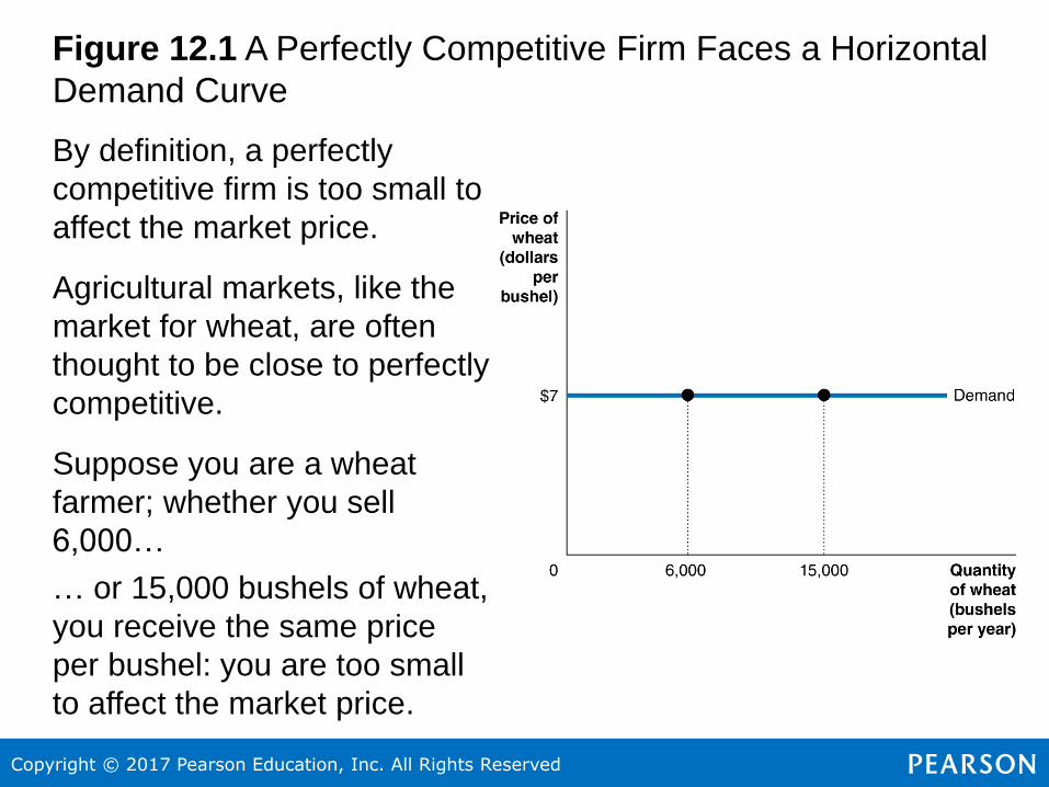
Figure 12.1 A Perfectly Competitive Firm Faces a Horizontal
Demand Curve
By definition, a perfectly
competitive firm is too small to
affect the market price.
Agricultural markets, like the
market for wheat, are often
thought to be close to perfectly
competitive.
Suppose you are a wheat
farmer; whether you sell
6,000…
… or 15,000 bushels of wheat,
you receive the same price
per bushel: you are too small
to affect the market price.
Copyright © 2017 Pearson Education, Inc. All Rights Reserved
7
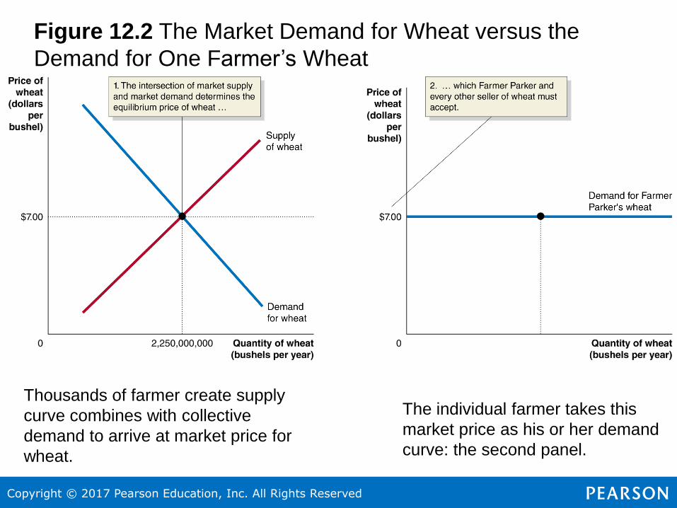
Figure 12.2 The Market Demand for Wheat versus the
Demand for One Farmer’s Wheat
The individual farmer takes this
market price as his or her demand
curve: the second panel.
Thousands of farmer create supply
curve combines with collective
demand to arrive at market price for
wheat.
Copyright © 2017 Pearson Education, Inc. All Rights Reserved
8
A very large number of small sellers who sell identical
products imply
A) a multitude of vastly different selling prices.
B) a downward sloping demand curve for each seller's
product.
C) the inability of one seller to influence price.
D) chaos in the market. C
Copyright © 2017 Pearson Education, Inc. All Rights Reserved
99
12.2 How a Firm Maximizes Profit in a
Perfect Competitive MarketExplain how a firm maximizes profit in a perfectly competitive market.
Assumption all firms try to maximize profits—including perfectly
competitive ones.
Profit = Total Revenue − Total Cost
Revenue for a perfectly competitive firm is easy: the firm receives
the same amount of money for every unit of output it sells.
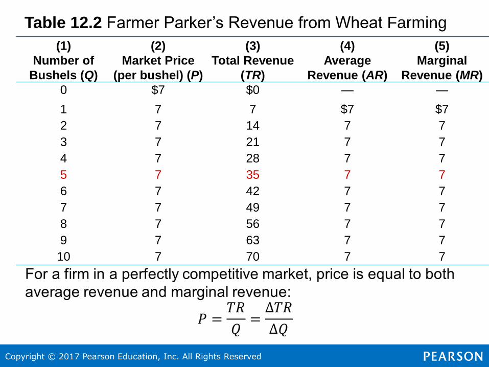
Price = Average Revenue = Marginal Revenue
Average revenue (AR) is total revenue divided by the quantity of
the product sold; Marginal revenue (MR) is the change in total
revenue from selling one more unit of a product.
Copyright © 2017 Pearson Education, Inc. All Rights Reserved
10
Table 12.2 Farmer Parker’s Revenue from Wheat Farming
(1)
Number of
Bushels (Q)
(2)
Market Price
(per bushel) (P)
(3)
Total Revenue
(TR)
(4)
Average
Revenue (AR)
(5)
Marginal
Revenue (MR)
0 $7 $0 — —
1 7 7 $7 $7
2 7 14 7 7
3 7 21 7 7
4 7 28 7 7
5 7 35 7 7
6 7 42 7 7
7 7 49 7 7
8 7 56 7 7
9 7 63 7 7
10 7 70 7 7
Copyright © 2017 Pearson Education, Inc. All Rights Reserved
1111
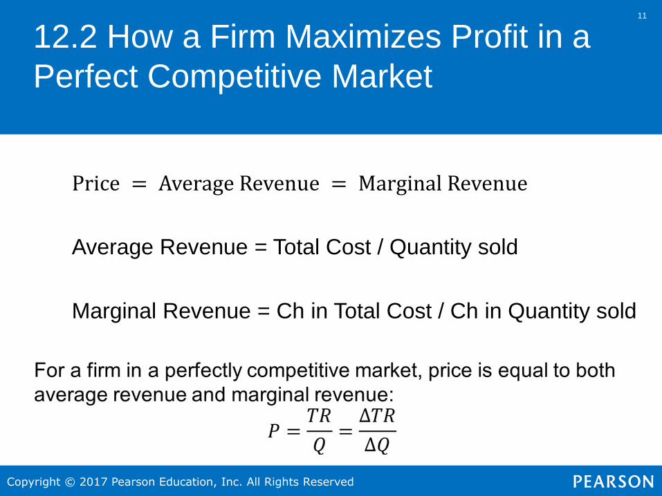
12.2 How a Firm Maximizes Profit in a
Perfect Competitive Market
Price = Average Revenue = Marginal Revenue
Average Revenue = Total Cost / Quantity sold
Marginal Revenue = Ch in Total Cost / Ch in Quantity sold
Copyright © 2017 Pearson Education, Inc. All Rights Reserved
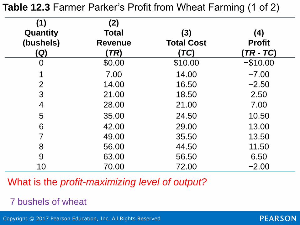
12Table 12.3 Farmer Parker’s Profit from Wheat Farming (1 of 2)
(1)
Quantity
(bushels)
(Q)
(2)
Total
Revenue
(TR)
(3)
Total Cost
(TC)
(4)
Profit
(TR - TC)
0 $0.00 $10.00 −$10.00
1 7.00 14.00 −7.00
2 14.00 16.50 −2.50
3 21.00 18.50 2.50
4 28.00 21.00 7.00
5 35.00 24.50 10.50
6 42.00 29.00 13.00
7 49.00 35.50 13.50
8 56.00 44.50 11.50
9 63.00 56.50 6.50
10 70.00 72.00 −2.00
What is the profit-maximizing level of output?
7 bushels of wheat
Copyright © 2017 Pearson Education, Inc. All Rights Reserved
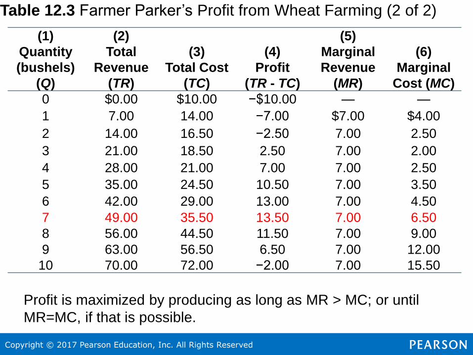
13Table 12.3 Farmer Parker’s Profit from Wheat Farming (2 of 2)
(1)
Quantity
(bushels)
(Q)
(2)
Total
Revenue
(TR)
(3)
Total Cost
(TC)
(4)
Profit
(TR - TC)
(5)
Marginal
Revenue
(MR)
(6)
Marginal
Cost (MC)
0 $0.00 $10.00 −$10.00 — —
1 7.00 14.00 −7.00 $7.00 $4.00
2 14.00 16.50 −2.50 7.00 2.50
3 21.00 18.50 2.50 7.00 2.00
4 28.00 21.00 7.00 7.00 2.50
5 35.00 24.50 10.50 7.00 3.50
6 42.00 29.00 13.00 7.00 4.50
7 49.00 35.50 13.50 7.00 6.50
8 56.00 44.50 11.50 7.00 9.00
9 63.00 56.50 6.50 7.00 12.00
10 70.00 72.00 −2.00 7.00 15.50
Profit is maximized by producing as long as MR > MC; or until
MR=MC, if that is possible.
Copyright © 2017 Pearson Education, Inc. All Rights Reserved
14
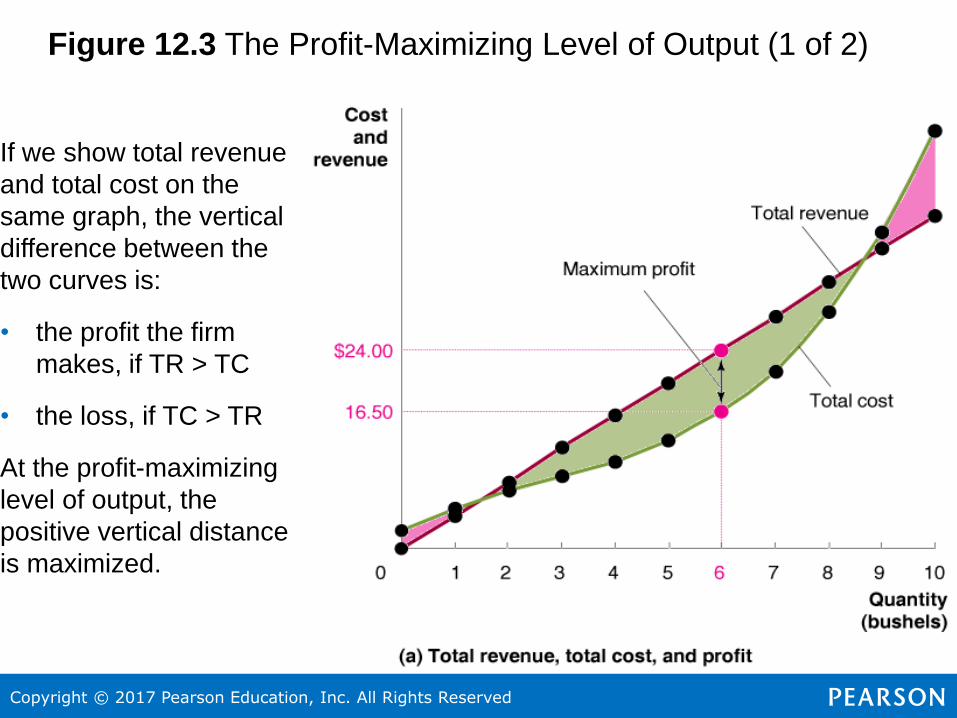
Figure 12.3 The Profit-Maximizing Level of Output (1 of 2)
If we show total revenue
and total cost on the
same graph, the vertical
difference between the
two curves is:
• the profit the firm
makes, if TR > TC
• the loss, if TC > TR
At the profit-maximizing
level of output, the
positive vertical distance
is maximized.
Copyright © 2017 Pearson Education, Inc. All Rights Reserved
15
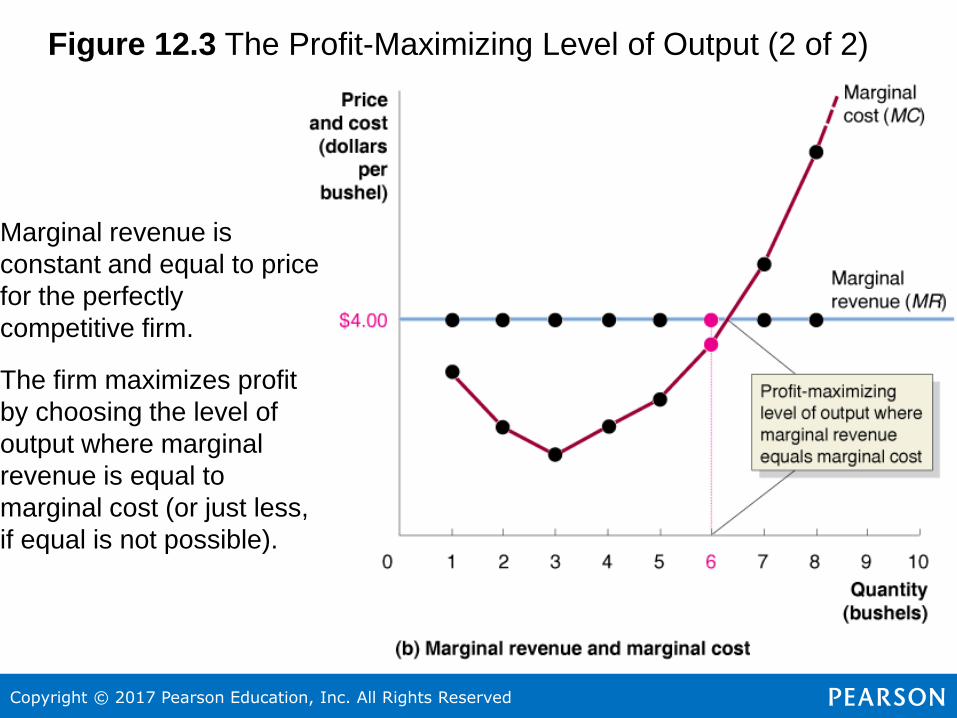
Figure 12.3 The Profit-Maximizing Level of Output (2 of 2)
Marginal revenue is
constant and equal to price
for the perfectly
competitive firm.
The firm maximizes profit
by choosing the level of
output where marginal
revenue is equal to
marginal cost (or just less,
if equal is not possible).
Copyright © 2017 Pearson Education, Inc. All Rights Reserved
16
Rules for Profit Maximization
The rules we have just developed for profit maximization are:
1. The profit-maximizing level of output is where the difference
between total revenue and total cost is greatest, and
2. The profit-maximizing level of output is also where MR = MC.
However neither of these rules require the assumption of perfect
competition; they are true for every firm!
For perfectly competitive firms, we can develop an additional rule,
because for those firms, P = MR; this implies:
3. The profit-maximizing level of output is also where P = MR.
Copyright © 2017 Pearson Education, Inc. All Rights Reserved
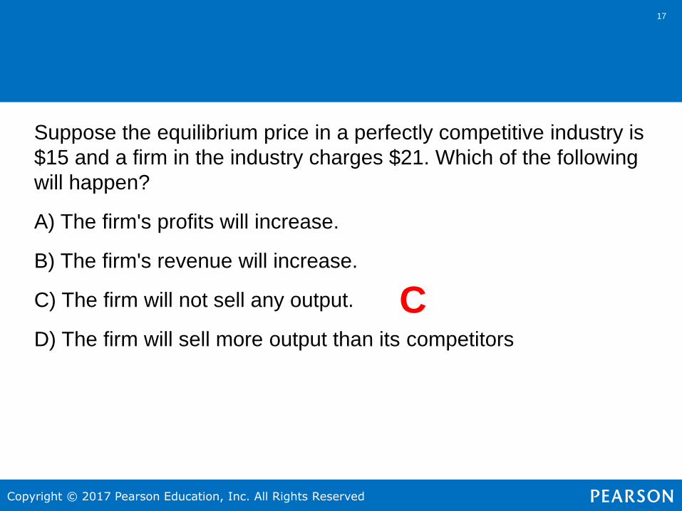
17
Suppose the equilibrium price in a perfectly competitive industry is
$15 and a firm in the industry charges $21. Which of the following
will happen?
A) The firm's profits will increase.
B) The firm's revenue will increase.
C) The firm will not sell any output.
D) The firm will sell more output than its competitors
C
Copyright © 2017 Pearson Education, Inc. All Rights Reserved
18
If the market price is $25, the average revenue of selling five units
is
A) $125.
B) $25.
C) $12.50.
D) $5.
B; AR = TR / Q
Copyright © 2017 Pearson Education, Inc. All Rights Reserved
19
If the market price is $25 in a perfectly competitive market, the
marginal revenue from selling the fifth unit is
A) $5.
B) $12.50.
C) $25.
D) $125.C;
MR = Ch in TR / Ch in Q
Price = AR = MR
Copyright © 2017 Pearson Education, Inc. All Rights Reserved
2020
12.3 Illustrating Profit or Loss on the
Cost Curve GraphUse graphs to show a firm’s profit or loss.
We know profit equals total revenue minus total cost, and total
revenue is price times quantity.
Profit = 𝑃 × 𝑄 − 𝑇𝐶
Divide both sides by Q:Profit
𝑄=𝑃 × 𝑄
𝑄−𝑇𝐶
𝑄Profit
𝑄= 𝑃 − 𝐴𝑇𝐶
Multiply both sides by Q:
Profit = 𝑃 − 𝐴𝑇𝐶 × 𝑄
The right hand side is the area of a rectangle with height (𝑃 −𝐴𝑇𝐶) and length 𝑄. We can use this to illustrate profit on a graph.

Copyright © 2017 Pearson Education, Inc. All Rights Reserved
21Figure 12.4 The Area of Maximum Profit (1 of 2)
A firm maximizes profit at
the level of output at
which MR = MC.
The difference between
price and average total
cost equals profit per unit
of output.
Total profit equals profit
per unit of output, times
the amount of output: the
area of the green
rectangle on the graph.
Copyright © 2017 Pearson Education, Inc. All Rights Reserved
22
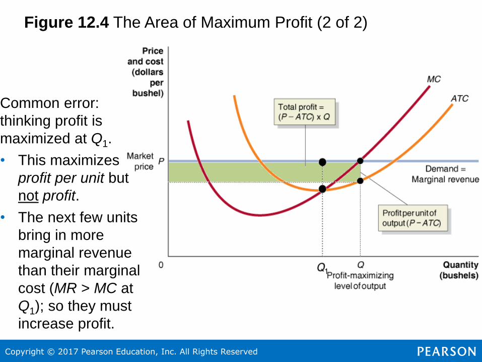
Figure 12.4 The Area of Maximum Profit (2 of 2)
Common error:
thinking profit is
maximized at Q1.
• This maximizes
profit per unit but
not profit.
• The next few units
bring in more
marginal revenue
than their marginal
cost (MR > MC at
Q1); so they must
increase profit.
Copyright © 2017 Pearson Education, Inc. All Rights Reserved
23
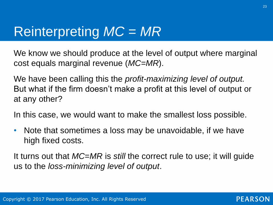
Reinterpreting MC = MR
We know we should produce at the level of output where marginal
cost equals marginal revenue (MC=MR).
We have been calling this the profit-maximizing level of output.
But what if the firm doesn’t make a profit at this level of output or
at any other?
In this case, we would want to make the smallest loss possible.
• Note that sometimes a loss may be unavoidable, if we have
high fixed costs.
It turns out that MC=MR is still the correct rule to use; it will guide
us to the loss-minimizing level of output.
Copyright © 2017 Pearson Education, Inc. All Rights Reserved
24
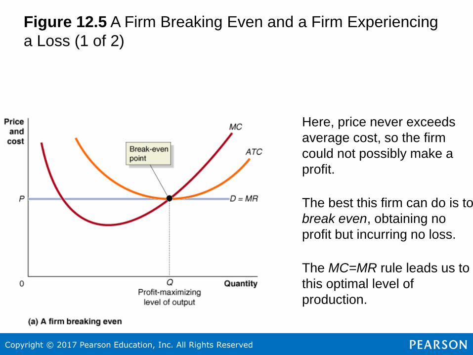
Figure 12.5 A Firm Breaking Even and a Firm Experiencing
a Loss (1 of 2)
Here, price never exceeds
average cost, so the firm
could not possibly make a
profit.
The best this firm can do is to
break even, obtaining no
profit but incurring no loss.
The MC=MR rule leads us to
this optimal level of
production.
Copyright © 2017 Pearson Education, Inc. All Rights Reserved
25
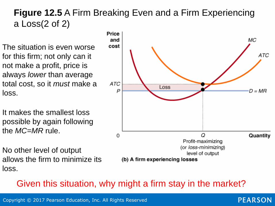
Figure 12.5 A Firm Breaking Even and a Firm Experiencing
a Loss(2 of 2)
The situation is even worse
for this firm; not only can it
not make a profit, price is
always lower than average
total cost, so it must make a
loss.
It makes the smallest loss
possible by again following
the MC=MR rule.
No other level of output
allows the firm to minimize its
loss.
Given this situation, why might a firm stay in the market?
Copyright © 2017 Pearson Education, Inc. All Rights Reserved
26
Identifying Whether a Firm Can Make a
Profit
Once we have determined the quantity where MC=MR, we can
immediately know whether the firm is making a profit, breaking
even, or making a loss. At that quantity,
• If P > ATC, the firm is making a profit
• If P = ATC, the firm is breaking even
• If P < ATC, the firm is making a loss
These statements hold true at every level of output.
Copyright © 2017 Pearson Education, Inc. All Rights Reserved
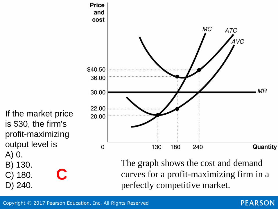
27
The graph shows the cost and demand
curves for a profit-maximizing firm in a
perfectly competitive market.
If the market price
is $30, the firm's
profit-maximizing
output level is
A) 0.
B) 130.
C) 180.
D) 240.C
Copyright © 2017 Pearson Education, Inc. All Rights Reserved
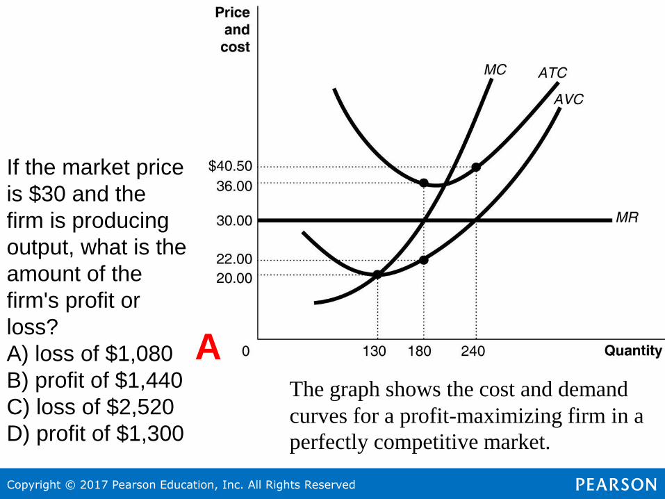
28
The graph shows the cost and demand
curves for a profit-maximizing firm in a
perfectly competitive market.
If the market price
is $30 and the
firm is producing
output, what is the
amount of the
firm's profit or
loss?
A) loss of $1,080
B) profit of $1,440
C) loss of $2,520
D) profit of $1,300
A
Copyright © 2017 Pearson Education, Inc. All Rights Reserved
2929
12.4 Deciding Whether to Produce or to
Shut Down in the Short RunExplain why firms may shut down temporarily.
Suppose a firm in a perfectly competitive market is making a loss.
It would like the price to be higher, but it is a price-taker, so it
cannot raise the price. That leaves two options:
1. Continue to produce, or
2. Stop production by shutting down temporarily
If the firm shuts down, it will still need to pay its fixed costs. The
firm needs to decide whether to incur only its fixed costs or to
produce and incur some variable costs, but obtain some revenue.
Fixed costs should be ignored because they are sunk costs, costs
that have already been paid and cannot be recovered; even if they
haven’t literally been paid yet, the firm is still obliged to pay them.
Example?
Copyright © 2017 Pearson Education, Inc. All Rights Reserved
30
The Supply Curve of a Firm in the Short
RunThe firm’s shut down decision is based on its variable costs; it
should produce nothing only if:
Total Revenue < Variable Cost
(P x Q) < VC
Dividing both sides by Q, we obtain:
P < AVC
So if P < AVC, the firm should produce 0 units of output.
If P ≥ AVC, then the MC = MR rule guides production: produce the
quantity where MC = MR. For a perfectly competitive firm, this
means where MC = P.
• So the marginal cost curve gives us the relationship between
price and quantity supplied: it is the firm’s supply curve!
Copyright © 2017 Pearson Education, Inc. All Rights Reserved
31
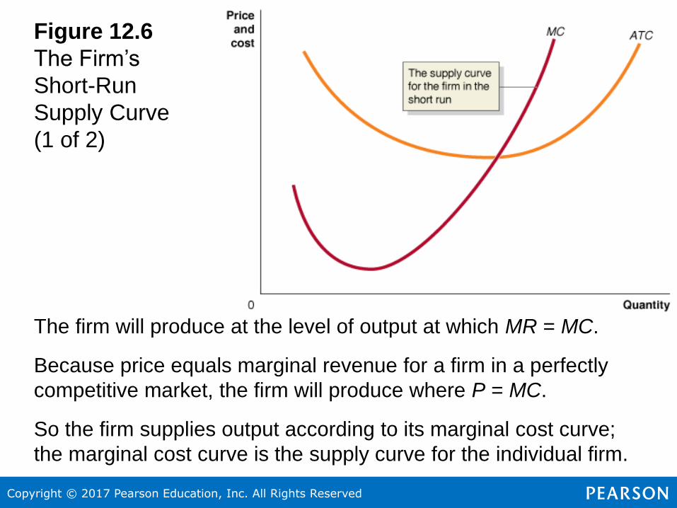
Figure 12.6
The Firm’s
Short-Run
Supply Curve
(1 of 2)
The firm will produce at the level of output at which MR = MC.
Because price equals marginal revenue for a firm in a perfectly
competitive market, the firm will produce where P = MC.
So the firm supplies output according to its marginal cost curve;
the marginal cost curve is the supply curve for the individual firm.
Copyright © 2017 Pearson Education, Inc. All Rights Reserved
32
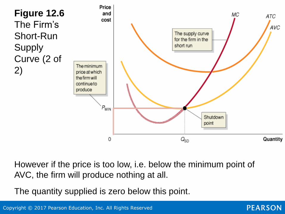
Figure 12.6
The Firm’s
Short-Run
Supply
Curve (2 of
2)
However if the price is too low, i.e. below the minimum point of
AVC, the firm will produce nothing at all.
The quantity supplied is zero below this point.
Copyright © 2017 Pearson Education, Inc. All Rights Reserved
33
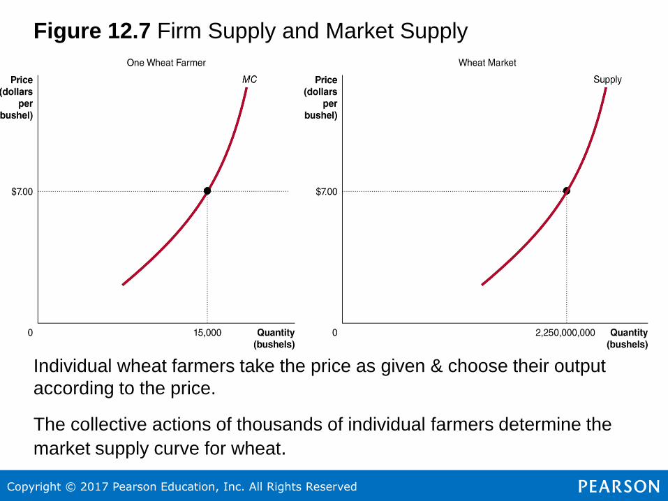
Figure 12.7 Firm Supply and Market Supply
Individual wheat farmers take the price as given & choose their output
according to the price.
The collective actions of thousands of individual farmers determine the
market supply curve for wheat.
Copyright © 2017 Pearson Education, Inc. All Rights Reserved
34
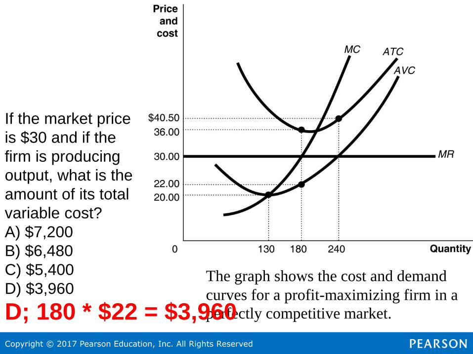
The graph shows the cost and demand
curves for a profit-maximizing firm in a
perfectly competitive market.
If the market price
is $30 and if the
firm is producing
output, what is the
amount of its total
variable cost?
A) $7,200
B) $6,480
C) $5,400
D) $3,960
D; 180 * $22 = $3,960
Copyright © 2017 Pearson Education, Inc. All Rights Reserved
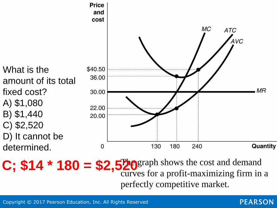
35
The graph shows the cost and demand
curves for a profit-maximizing firm in a
perfectly competitive market.
What is the
amount of its total
fixed cost?
A) $1,080
B) $1,440
C) $2,520
D) It cannot be
determined.
C; $14 * 180 = $2,520
Copyright © 2017 Pearson Education, Inc. All Rights Reserved
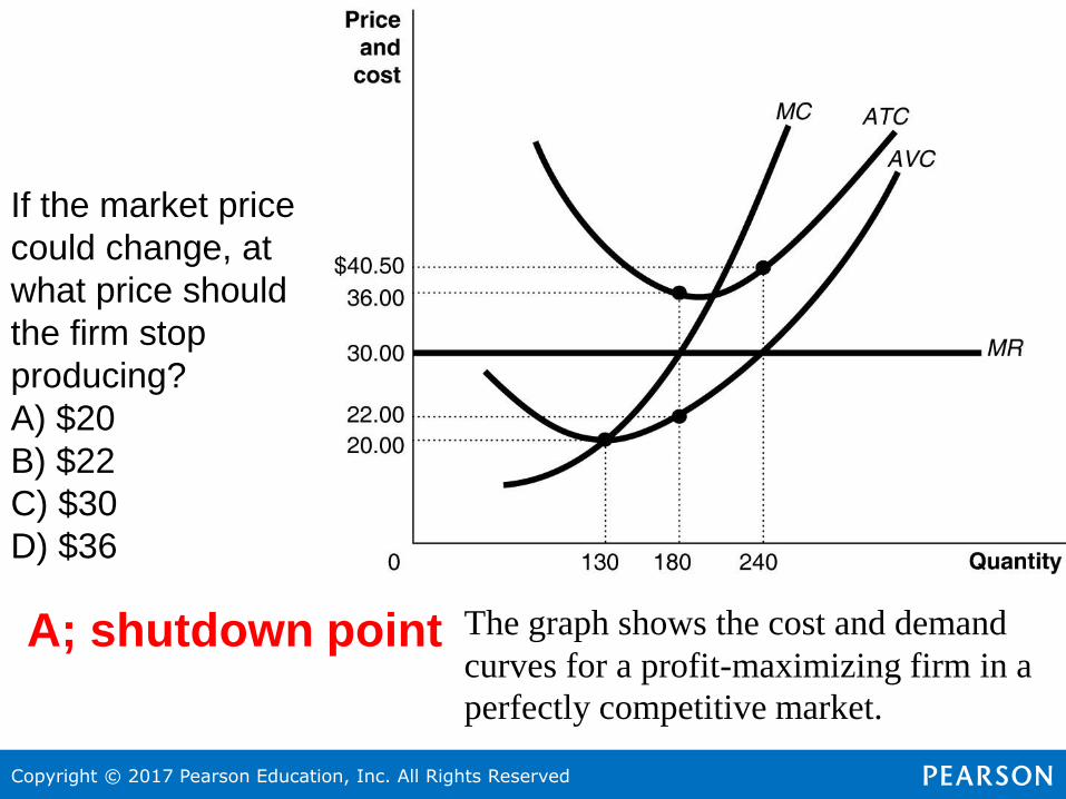
36
The graph shows the cost and demand
curves for a profit-maximizing firm in a
perfectly competitive market.
If the market price
could change, at
what price should
the firm stop
producing?
A) $20
B) $22
C) $30
D) $36
A; shutdown point
Copyright © 2017 Pearson Education, Inc. All Rights Reserved
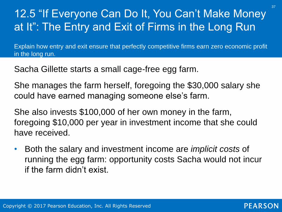
3737
12.5 “If Everyone Can Do It, You Can’t Make Money
at It”: The Entry and Exit of Firms in the Long Run
Explain how entry and exit ensure that perfectly competitive firms earn zero economic profit
in the long run.
Sacha Gillette starts a small cage-free egg farm.
She manages the farm herself, foregoing the $30,000 salary she
could have earned managing someone else’s farm.
She also invests $100,000 of her own money in the farm,
foregoing $10,000 per year in investment income that she could
have received.
• Both the salary and investment income are implicit costs of
running the egg farm: opportunity costs Sacha would not incur
if the farm didn’t exist.
Copyright © 2017 Pearson Education, Inc. All Rights Reserved
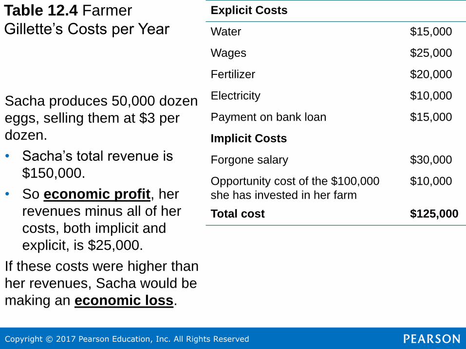
38Table 12.4 Farmer
Gillette’s Costs per Year
Sacha produces 50,000 dozen
eggs, selling them at $3 per
dozen.
• Sacha’s total revenue is
$150,000.
• So economic profit, her
revenues minus all of her
costs, both implicit and
explicit, is $25,000.
If these costs were higher than
her revenues, Sacha would be
making an economic loss.
Explicit Costs Blank
Water $15,000
Wages $25,000
Fertilizer $20,000
Electricity $10,000
Payment on bank loan $15,000
Implicit Costs Blank
Forgone salary $30,000
Opportunity cost of the $100,000
she has invested in her farm
$10,000
Total cost $125,000
Copyright © 2017 Pearson Education, Inc. All Rights Reserved
39
Economic Profit Leads to Entry of New
Firms
Unfortunately for Sacha, the profits in the egg-farming business
will not last. Why?
Additional firms will enter the market, attracted by the profit.
• Some farms will switch from other products to cage-free eggs,
OR
• People will open up new farms.
However it happens, the number of firms in the market will
increase, increasing supply; this will in turn lower the price Sacha
can receive for her output.
Copyright © 2017 Pearson Education, Inc. All Rights Reserved
40
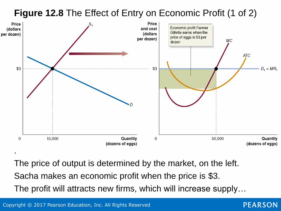
Figure 12.8 The Effect of Entry on Economic Profit (1 of 2)
.
The price of output is determined by the market, on the left.
Sacha makes an economic profit when the price is $3.
The profit will attracts new firms, which will increase supply…
Copyright © 2017 Pearson Education, Inc. All Rights Reserved
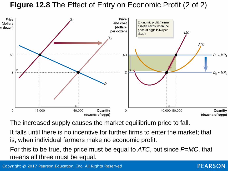
41Figure 12.8 The Effect of Entry on Economic Profit (2 of 2)
The increased supply causes the market equilibrium price to fall.
It falls until there is no incentive for further firms to enter the market; that
is, when individual farmers make no economic profit.
For this to be true, the price must be equal to ATC, but since P=MC, that
means all three must be equal.
Copyright © 2017 Pearson Education, Inc. All Rights Reserved
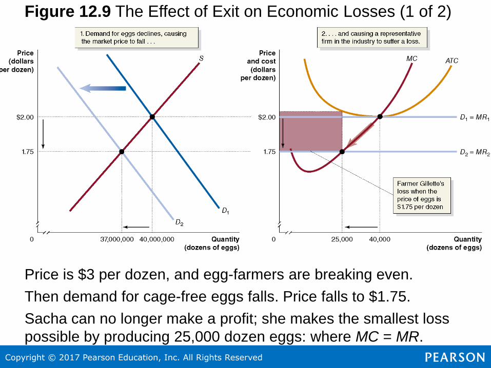
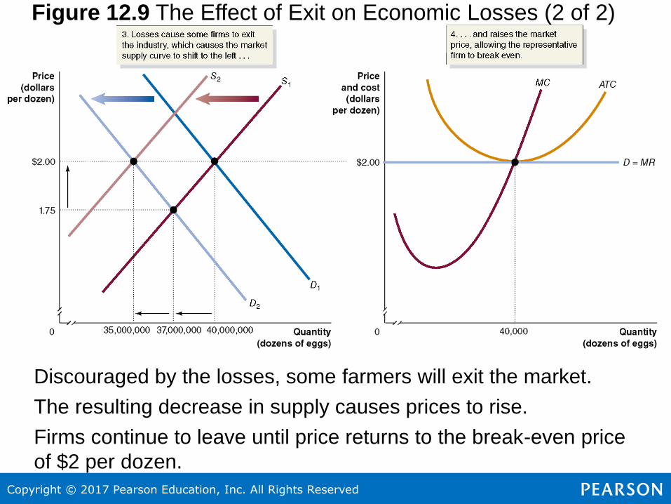
42Figure 12.9 The Effect of Exit on Economic Losses (1 of 2)
Price is $3 per dozen, and egg-farmers are breaking even.
Then demand for cage-free eggs falls. Price falls to $1.75.
Sacha can no longer make a profit; she makes the smallest loss
possible by producing 25,000 dozen eggs: where MC = MR.
Copyright © 2017 Pearson Education, Inc. All Rights Reserved
43Figure 12.9 The Effect of Exit on Economic Losses (2 of 2)
Discouraged by the losses, some farmers will exit the market.
The resulting decrease in supply causes prices to rise.
Firms continue to leave until price returns to the break-even price
of $2 per dozen.
Copyright © 2017 Pearson Education, Inc. All Rights Reserved
44
Long-Run Equilibrium in a Perfectly
Competitive MarketThe previous slides have described how long-run competitive
equilibrium is achieved in a perfectly competitive market:
• If firms are making an economic profit, additional firms enter the
market, driving down price to the break-even level.
• If firms are making an economic loss, existing firms exit the
market, driving price up to the break-even level.
Since the long-run average cost curve shows the lowest cost at
which a firm is able to produce a given quantity of output in the
long run, we expect price to be driven down to the minimum point
on the typical firm’s long-run average cost curve.
Long-run competitive equilibrium: The situation in which the
entry and exit of firms has resulted in the typical firm breaking
even.
Copyright © 2017 Pearson Education, Inc. All Rights Reserved
45
Long-Run Market Supply in a Perfectly
Competitive Market
This means that in the long run, the market will supply any
demand by consumers at a price equal to the minimum point on
the typical firm’s average cost curve.
• So the long-run supply curve is horizontal at this price.
• In a perfectly competitive market, the long-run price is
completely determined by the forces of supply.
• The number of suppliers adjusts to meet demand, at the lowest
possible price.
Long-run supply curve: A curve that shows the relationship in
the long run between market price and the quantity supplied.
Copyright © 2017 Pearson Education, Inc. All Rights Reserved
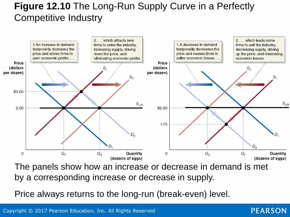
46Figure 12.10 The Long-Run Supply Curve in a Perfectly
Competitive Industry
The panels show how an increase or decrease in demand is met
by a corresponding increase or decrease in supply.
Price always returns to the long-run (break-even) level.

Copyright © 2017 Pearson Education, Inc. All Rights Reserved
47
Making the Connection: Easy Entry
Makes the Long Run Pretty Short (1 of 2)
When firms earn economic profits
in a market, other firms have a
strong economic incentive to
enter that market.
This is exactly what happened
with iPhone apps, first provided
by Apple in mid-2008. Proving to
be highly profitable in an instant,
more than 25,000 apps were
available in the iTunes store
within a year.

Copyright © 2017 Pearson Education, Inc. All Rights Reserved
48
Making the Connection: Easy Entry
Makes the Long Run Pretty Short (2 of 2)
The cost of entering this market
was very small. Anyone with the
programming skills and the time
to write an app could have it
posted in the store.
As a result of this enhanced
competition, the ability to get rich
quick with a killer app faded
quickly.
Copyright © 2017 Pearson Education, Inc. All Rights Reserved
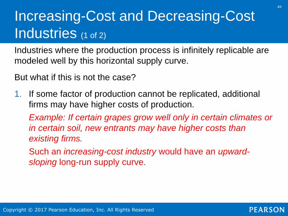
49
Increasing-Cost and Decreasing-Cost
Industries (1 of 2)
Industries where the production process is infinitely replicable are
modeled well by this horizontal supply curve.
But what if this is not the case?
1. If some factor of production cannot be replicated, additional
firms may have higher costs of production.
Example: If certain grapes grow well only in certain climates or
in certain soil, new entrants may have higher costs than
existing firms.
Such an increasing-cost industry would have an upward-
sloping long-run supply curve.
Copyright © 2017 Pearson Education, Inc. All Rights Reserved
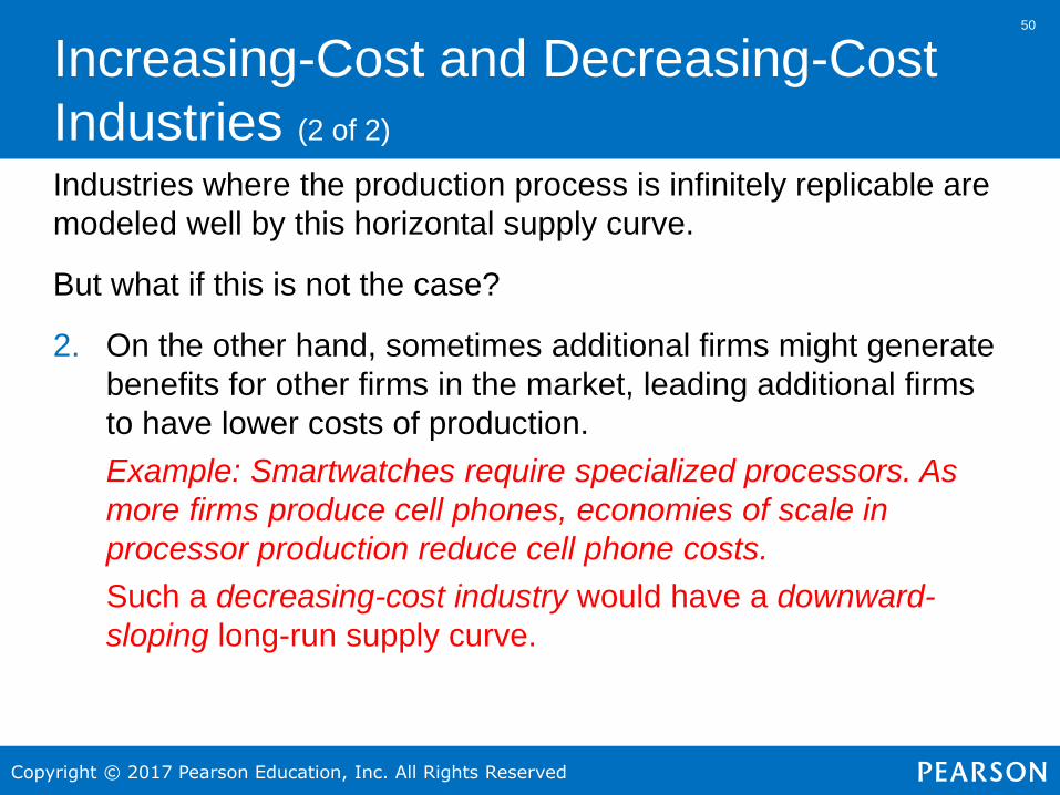
50
Increasing-Cost and Decreasing-Cost
Industries (2 of 2)
Industries where the production process is infinitely replicable are
modeled well by this horizontal supply curve.
But what if this is not the case?
2. On the other hand, sometimes additional firms might generate
benefits for other firms in the market, leading additional firms
to have lower costs of production.
Example: Smartwatches require specialized processors. As
more firms produce cell phones, economies of scale in
processor production reduce cell phone costs.
Such a decreasing-cost industry would have a downward-
sloping long-run supply curve.
Copyright © 2017 Pearson Education, Inc. All Rights Reserved
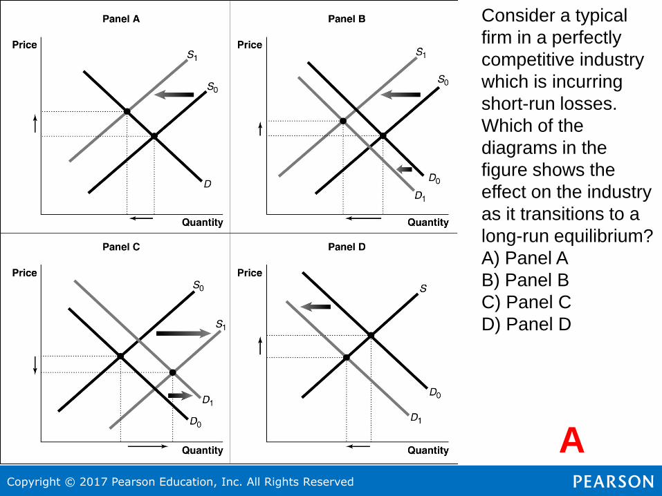
51Consider a typical
firm in a perfectly
competitive industry
which is incurring
short-run losses.
Which of the
diagrams in the
figure shows the
effect on the industry
as it transitions to a
long-run equilibrium?
A) Panel A
B) Panel B
C) Panel C
D) Panel D
A
Copyright © 2017 Pearson Education, Inc. All Rights Reserved
5252
12.6 Perfect Competition and Efficiency
Explain how perfect competition leads to economic efficiency.
Efficiency in economics refers to two separate but related
concepts:
Productive efficiency is a situation in which a good or service is
produced at the lowest possible cost.
Allocative efficiency is a state of the economy in which
production represents consumer preferences; in particular, every
good or service is produced up to the point where the last unit
provides a marginal benefit to consumers equal to the marginal
cost of producing it.
Copyright © 2017 Pearson Education, Inc. All Rights Reserved
53
Are Perfectly Competitive Markets
Efficient?
We have shown that in the long run, perfectly competitive markets are
productively efficient.
But they are allocatively efficient also:
1. The price of a good represents the marginal benefit consumers
receive from consuming the last unit of the good sold.
2. Perfectly competitive firms produce up to the point where the price
of the good equals the marginal cost of producing the good.
3. Therefore, firms produce up to the point where the last unit
provides a marginal benefit to consumers equal to the marginal
cost of producing it.
Productive and allocative efficiency are useful benchmarks against
which to measure the actual performance of other markets.