chapter 13: multiple regressioncparrish.sewanee.edu/stat204 s2015/notes/part 04...

Stat 204, Part 4 Association

Chapter 13: Multiple Regression

These notes reflect material from our text, Statistics: The Art and Science of Learning from Data,Third Edition, by Alan Agresti and Catherine Franklin, published by Pearson, 2013.

Multiple Regression

Imagine a three-dimensional space with coordinates (x1, x2, y). We illustrate the idea of multiple re-gression by creating some data points which seem to arrange themselves near a plane hovering above thex1−x2 coordinate plane. It is the goal of multiple regression to calculate the plane which best fits that data.

Each data point has coordinates of the form (x1, x2, y), and for each set of coordinates (x1, x2, 0) in thecoordinate plane down below, R’s lm predicts the average height y above the x1 − x2 coordinate plane ofall the data points having those first two coordinates. All points of the form (x1, x2, y) lie in a plane whichwe describe as the plane best fitting the data.

First, construct 200 data points which very nearly satisfy the equation y = 10 + x1 + 2x2 except forsmall random perturbations (Kruschke, 2015, p.511).

# data

x1 <- runif(200, min = 0, max = 10)

x2 <- runif(200, min = 0, max = 10)

e <- rnorm(200, 0, 2.0)

y <- 10 + 1 * x1 + 2 * x2 + e

pairs(y ~ x1 + x2, Data,

col = "darkred")

y

0 2 4 6 8 10

1015

2025

3035

40

02

46

810

x1

10 15 20 25 30 35 40 0 2 4 6 8 10

02

46

810

x2

Spring 2015 of 20


Now, use predict to calculate the best-fitting plane from the data.

Data <- data.frame(x1, x2, y)

Data.lm <- lm(y ~ x1 + x2, data = Data)

predict.y.hat <- function(x1, x2){

predict(Data.lm, data.frame(x1 = x1, x2 = x2))

}

x3 <- x4 <- seq(0, 10, 0.5) # grid

y.hat <- outer(x3, x4, predict.y.hat) # predicted y.hat’s

persp(x3, x4, y.hat, theta = 20, phi = 20,

r = 20, zlim = c(0, 50),

ticktype = ’detailed’, col = "mintcream",

xlab = ’x1’, ylab = ’x2’, zlab = ’y’) -> res # capture the perspective matrix

points(trans3d(x1, x2, y, pm = res),

col="darkred", pch=19)

x1

0 2 4 6 8 10

x2

0246810

y

0

10

20

30

40

50

In one such experiment, the best-fitting plane had equation

y = 9.645338 + 1.080860× x1 + 1.979942× x2,

which is reasonably close to the equation y = 10 + x1 + 2x2 used to generate the data.

Spring 2015 of 20


House Prices

HP.in.thousands

2000 6000 10000

0200

400

600

800

2000

6000

10000

House.Size

0 200 400 600 800 0 2 4 6 8

02

46

8

Bedrooms

Multiple linear regression

Multiple linear regression creates a linear model with k explanatory variables.

y = β0 + β1x1 + · · ·+ βkxk

Highly correlated explanatory variables are to be avoided.

Inference : Are all the β’s equal to 0? ... F test

Inference : If not all the β’s are equal to 0, then which ones are not 0? ... t tests ... CIs for βi

Building a model : Either of two algorithms (forward or backward) can be used to systematically adduncorrelated variables or delete highly correlated variables to or from the developing model, with either por R2 ordering the addition or deletion of variables at each step

Conditions for multiple linear regression

Acorn size and oak tree range, eesee

Spring 2015 of 20


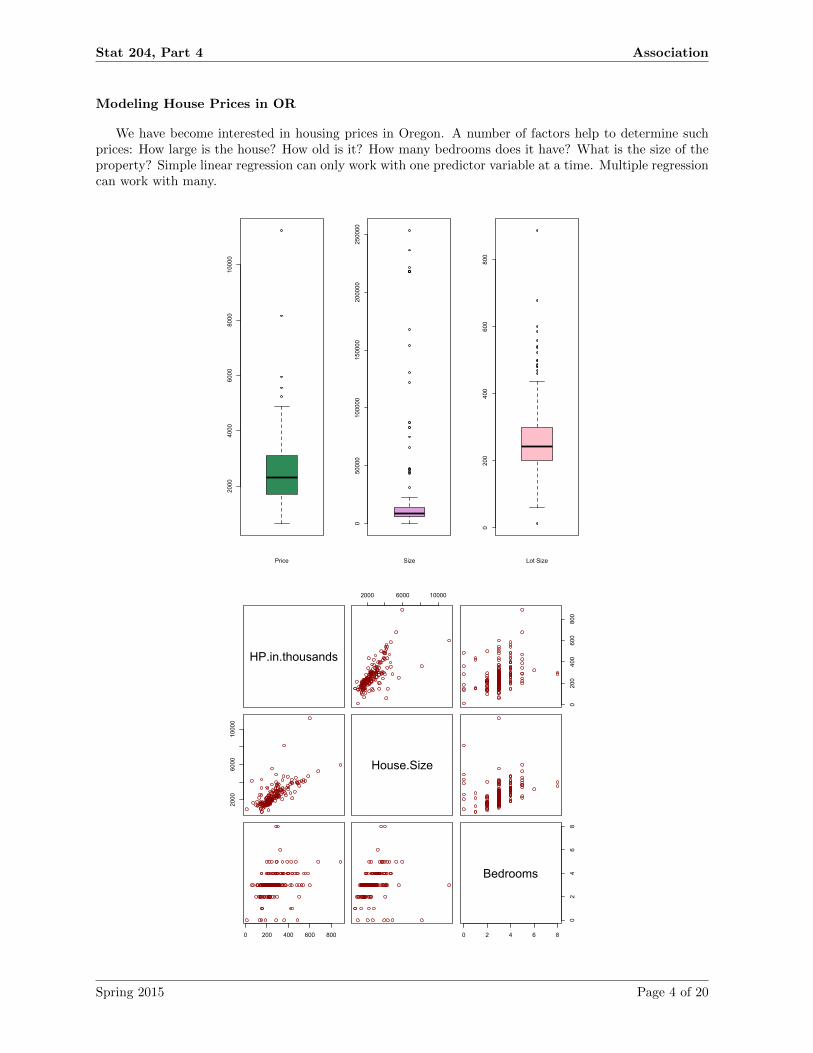
Modeling House Prices in OR

We have become interested in housing prices in Oregon. A number of factors help to determine suchprices: How large is the house? How old is it? How many bedrooms does it have? What is the size of theproperty? Simple linear regression can only work with one predictor variable at a time. Multiple regressioncan work with many.

2000

4000

6000

8000

10000

Price

050000

100000

150000

200000

250000

Size

0200

400

600

800

Lot Size

HP.in.thousands

2000 6000 10000

0200

400

600

800

2000

6000

10000

House.Size

0 200 400 600 800 0 2 4 6 8

02

46

8

Bedrooms

Spring 2015 of 20


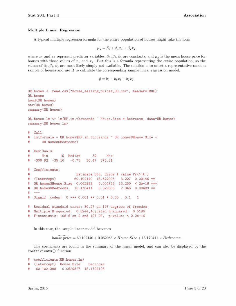
Multiple Linear Regression

A typical multiple regression formula for the entire population of houses might take the form

µy = β0 + β1x1 + β2x2,

where x1 and x2 represent predictor variables, β0, β1, β2 are constants, and µy is the mean house price forhouses with those values of x1 and x2. But this is a formula representing the entire population, so thevalues of β0, β1, β2 are most likely simply not available. The solution is to select a representative randomsample of houses and use R to calculate the corresponding sample linear regression model:

y = b0 + b1x1 + b2x2.

OR.homes <- read.csv("house_selling_prices_OR.csv", header=TRUE)

OR.homes

head(OR.homes)

str(OR.homes)

summary(OR.homes)

OR.homes.lm <- lm(HP.in.thousands ~ House.Size + Bedrooms, data=OR.homes)

summary(OR.homes.lm)

# Call:

# lm(formula = OR.homes$HP.in.thousands ~ OR.homes$House.Size +

# OR.homes$Bedrooms)

# Residuals:

# Min 1Q Median 3Q Max

# -306.92 -35.16 -0.75 30.47 376.81

# Coefficients:

# Estimate Std. Error t value Pr(>|t|)

# (Intercept) 60.102140 18.622905 3.227 0.00146 **

# OR.homes$House.Size 0.062983 0.004753 13.250 < 2e-16 ***

# OR.homes$Bedrooms 15.170411 5.329806 2.846 0.00489 **

# ---

# Signif. codes: 0 *** 0.001 ** 0.01 * 0.05 . 0.1 1

# Residual standard error: 80.27 on 197 degrees of freedom

# Multiple R-squared: 0.5244,Adjusted R-squared: 0.5196

# F-statistic: 108.6 on 2 and 197 DF, p-value: < 2.2e-16

In this case, the sample linear model becomes

house price = 60.102140 + 0.062983×House.Size+ 15.170411×Bedrooms.

The coefficients are found in the summary of the linear model, and can also be displayed by thecoefficients() function.

# coefficients(OR.homes.lm)

# (Intercept) House.Size Bedrooms

# 60.1021398 0.0629827 15.1704105

Spring 2015 of 20


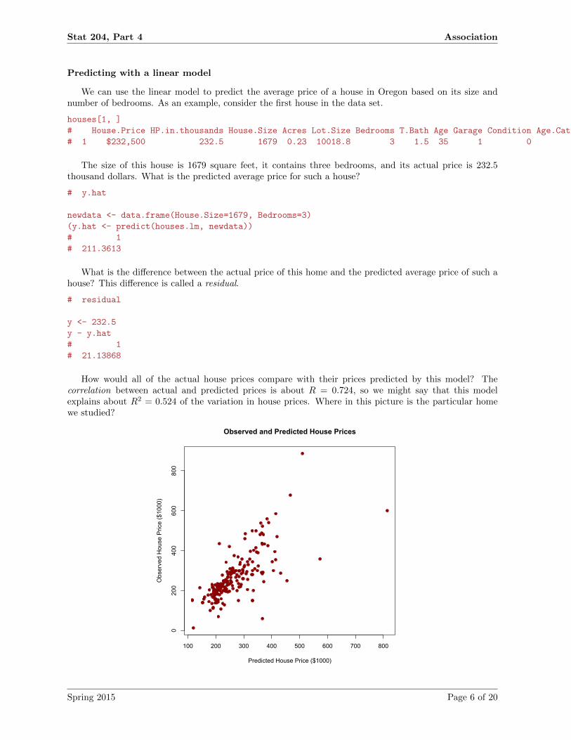
Predicting with a linear model

We can use the linear model to predict the average price of a house in Oregon based on its size andnumber of bedrooms. As an example, consider the first house in the data set.

houses[1, ]

# House.Price HP.in.thousands House.Size Acres Lot.Size Bedrooms T.Bath Age Garage Condition Age.Category

# 1 $232,500 232.5 1679 0.23 10018.8 3 1.5 35 1 0 M

The size of this house is 1679 square feet, it contains three bedrooms, and its actual price is 232.5thousand dollars. What is the predicted average price for such a house?

# y.hat

newdata <- data.frame(House.Size=1679, Bedrooms=3)

(y.hat <- predict(houses.lm, newdata))

# 1

# 211.3613

What is the difference between the actual price of this home and the predicted average price of such ahouse? This difference is called a residual.

# residual

y <- 232.5

y - y.hat

# 1

# 21.13868

How would all of the actual house prices compare with their prices predicted by this model? Thecorrelation between actual and predicted prices is about R = 0.724, so we might say that this modelexplains about R2 = 0.524 of the variation in house prices. Where in this picture is the particular homewe studied?

100 200 300 400 500 600 700 800

0200

400

600

800

Observed and Predicted House Prices

Predicted House Price ($1000)

Obs

erve

d H

ouse

Pric

e ($

1000

)

Spring 2015 of 20


Residuals

We can plot the observed prices against the predicted prices to explore the accuracy of such a model.The difference between the actual price of the ith house and its predicted price is the residual,

εi = yi − yi.

100 200 300 400 500 600 700 800

0200

400

600

800



Obs

erve

d H

ouse

Pric

e ($

1000

)

Linear regression requires that the residuals display a normal distribution.

House price residuals

residuals(houses.lm)

Frequency

-400 -200 0 200 400

020

4060

80

Spring 2015 of 20


Standardized Residuals

Standardized residuals are more informative than raw residuals. They are analogous to z-scores, in thatthey display how many standard errors, SE, the residual is from the mean.

House price standardized residuals

rstandard(houses.lm)

Frequency

-4 -2 0 2 4

020

4060

80

Crime, Education, and Urbanization

We turn now to a different study exploring possible relationships among crime, education rates, andurbanization in Florida.

crime

55 60 65 70 75 80 85

020

4060

80100

5560

6570

7580

85

education

0 20 40 60 80 100 0 20 40 60 80 100

020

4060

80100

urbanization

Spring 2015 of 20


Parallel Regression Lines

Import the data into R and calculate a linear model.

FL.crime <- read.csv("fl_crime.csv", header=TRUE)

head(FL.crime)

str(FL.crime)

summary(FL.crime)

FL.crime.subset <- subset(FL.crime, select=c("crime", "education","urbanization"))

FL.crime.lm <- lm(crime ~ education + urbanization, data=FL.crime.subset)

summary(FL.crime.lm)

Call:

lm(formula = crime ~ education + urbanization, data = FL.crime.subset)

# Residuals:


# -34.693 -15.742 -6.226 15.812 50.678

# Coefficients:


# (Intercept) 59.1181 28.3653 2.084 0.0411 *

# education -0.5834 0.4725 -1.235 0.2214

# urbanization 0.6825 0.1232 5.539 6.11e-07 ***

# ---

# Signif. codes: 0 *** 0.001 ** 0.01 * 0.05 . 0.1 1


# Multiple R-squared: 0.4714,Adjusted R-squared: 0.4549

# F-statistic: 28.54 on 2 and 64 DF, p-value: 1.379e-09

The sample linear model for this data is

crime = 59.1181− 0.5834× education+ 0.6825× urbanization.

0.0 0.2 0.4 0.6 0.8 1.0

050

100

150

Crime Rate in FL

Education

Crim

e R

ate

urbanization = 0crime rate = 59.12 - 0.5834 * education



Spring 2015 of 20


Interpreting Regression Output

Let’s dissect the output from that last linear model. Here is the code that produced the output. Thefirst line creates the model and the second displays a summary of its contents.

FL.crime.lm <- lm(crime ~ education + urbanization, data=FL.crime.subset)

summary(FL.crime.lm)

First, there is an echo of the call to create the model.

Call:

lm(formula = crime ~ education + urbanization, data = FL.crime.subset)

Then, a five-number summary indicating the distribution of the residuals ... Anything other thana normal distribution would be a sign of trouble, so we might complement these few statistics with ahistogram of the standardized residuals. Hmmm. What happened to the center of that distribution ofresiduals?

# Residuals:


# -34.693 -15.742 -6.226 15.812 50.678

FL Crime Standardized Residuals

rstandard(FL.crime.lm)

Frequency

-2 -1 0 1 2

05

1015

20

We assume a multiple regression model in the larger population,

µy = β0 + β1 × education+ β2 × urbanization.

Is the crime rate independent of the two predictors education and urbanization? This question can beframed as an hypothesis test.

H0 : β1 = β2 = 0

Ha : some βi is not 0.

The null hypothesis claims that the predictors are not associated with the response variable, and the al-ternative hypothesis says that at least one predictor is associated with the response variable.

Spring 2015 of 20


The test statistic for this hypothesis test on the basic relevance of the model is listed farther down inthe display as F = 28.54, with 2 and 64 degrees of freedom, and the associated p-value is very small indeed,so we reject the null hypothesis, accept the alternative hypothesis, and conclude that at least one of thepredictors is associated with the response variable.

# F-statistic: 28.54 on 2 and 64 DF, p-value: 1.379e-09

In this data set, there were n = 67 observations and g = 3 parameters (b0, b1, b2), so the degrees offreedom for the F distribution are df1 = g− 1 = 2 and df2 = n− g = 64. The p-value is the area under thecurve of the F distribution with 2 and 64 degrees of freedom and to the right of the F test statistic.

0 10 20 30 40

0.0

0.2

0.4

0.6

0.8

1.0

F TestAFS 13.5 FL crime

x

Density

F(df1 = 2, df2 = 64)

F = 28.54

p-value = 1.379e-09

The next question becomes “Which variable(s) is/are associated with the response variable?” The datain the section on Coefficients quantifies the relationships in our sample data. The numbers in the firstcolumn are the coefficients in the approximating sample prediction equation.

y = b0 + b1 × education+ b2 × urbanization= 59.1181− 0.5834× education+ 0.6825× urbanization.

The null hypothesis in our next test would be that the predictor urbanization and the response crimeare unrelated, so β2 = 0. We investigate this relationship with a t test. The point estimate of β2 isb2 = 0.6825, the standard error of that statistic is SE = 0.1232, the test statistic is t = b2/SE = 5.539,and the associated p-value is 6.11e-07. These numbers all come from the urbanization line in the Coef-ficients section of the output of the linear model. We reject the null hypothesis, accept the alternativehypothesis, and conclude that β2 6= 0, so crime and urbanization are associated.

Are crime and education associated? Is it plausible that β1 might be 0?

Spring 2015 of 20


The same statistics for urbanization can be used to construct a 95% confidence interval for β2.

CI = b2 ± t∗ × SE= 0.6825± 1.99773(0.1232)

→ [0.4363797, 0.9286203].

where t∗ was calculated with the r command qt(0.975, df=64). The degrees of freedom for the t distri-bution is n minus the number of parameters in the regression equation, which for this problem becomesn− 3 = 67− 3 = 64, which also figured as the second df in the F test.

# Coefficients:


# (Intercept) 59.1181 28.3653 2.084 0.0411 *

# education -0.5834 0.4725 -1.235 0.2214

# urbanization 0.6825 0.1232 5.539 6.11e-07 ***

# ---

# Signif. codes: 0 *** 0.001 ** 0.01 * 0.05 . 0.1 1

All of the conditional distributions of y given specific values of the predictors have normal distributionswith the same standard deviation, σ. The estimate of σ based on our sample data is the residual standarderror, RSE = 20.82.


The multiple R2 is the percent of the variation in y explained by the model, which in this case isR2 = 0.4714, indicating a rather loose relationship. Adding additional variables to the model wouldgenerally increase R2, even if the additional variables were essentially irrelevant, so some statisticians preferto use an adjusted R2 with a slightly different formula which penalizes the use of irrelevant variables.

# Multiple R-squared: 0.5244, Adjusted R-squared: 0.5196

FL Crime R2

R S

quar

ed

0.0

0.2

0.4

0.6

0.8

1.0

Spring 2015 of 20


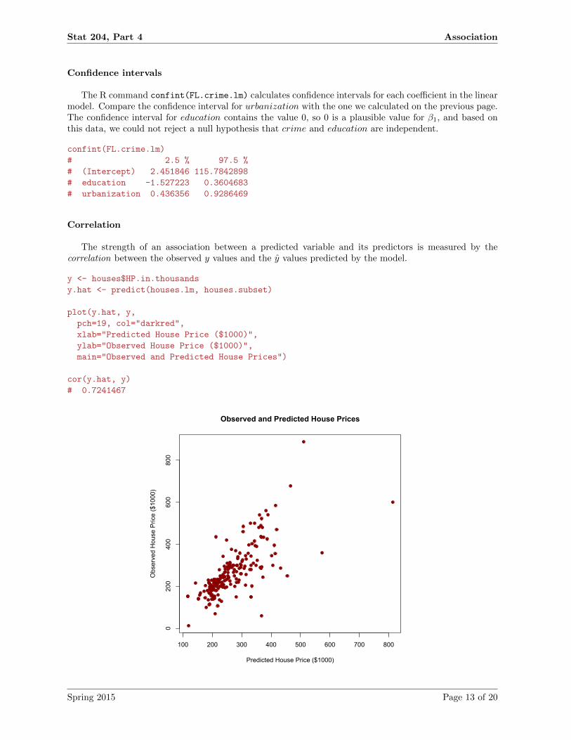
Confidence intervals

The R command confint(FL.crime.lm) calculates confidence intervals for each coefficient in the linearmodel. Compare the confidence interval for urbanization with the one we calculated on the previous page.The confidence interval for education contains the value 0, so 0 is a plausible value for β1, and based onthis data, we could not reject a null hypothesis that crime and education are independent.

confint(FL.crime.lm)

# 2.5 % 97.5 %

# (Intercept) 2.451846 115.7842898

# education -1.527223 0.3604683

# urbanization 0.436356 0.9286469

Correlation

The strength of an association between a predicted variable and its predictors is measured by thecorrelation between the observed y values and the y values predicted by the model.

y <- houses$HP.in.thousands

y.hat <- predict(houses.lm, houses.subset)

plot(y.hat, y,

pch=19, col="darkred",

xlab="Predicted House Price ($1000)",

ylab="Observed House Price ($1000)",

main="Observed and Predicted House Prices")

cor(y.hat, y)

# 0.7241467

100 200 300 400 500 600 700 800

0200

400

600

800



Obs

erve

d H

ouse

Pric

e ($

1000

)

Spring 2015 of 20


Correlation matrix

The same procedure can generate a matrix of correlations.

cor(FL.crime)

# crime income urbanization

# crime 1.0000000 0.4337503 0.6773678

# income 0.4337503 1.0000000 0.7306983

# urbanization 0.6773678 0.7306983 1.0000000

library(corrplot)

corrplot(cor(FL.crime.subset))

-1

-0.8

-0.6

-0.4

-0.2

0

0.2

0.4

0.6

0.8

1

crime

income

urbanization

crime

income

urbanization

Spring 2015 of 20


Building a Linear Model

Building a linear model is a fascinating enterprise best left to another statistics course, but one wayto proceed might be to first estimate the explanatory power, r2, of the separate variables, each one actingalone, and then add variables one-by-one to the growing model, monitoring the explanatory power of theaccumulating assemblage at each stage with R2. Note that R2 can only increase when we add a newvariable, but it may not increase by much.

House.Size Lot.Size Bedrooms T.Bath Age Garage

r^2 Values of Explanatory Variablesr s

quar

ed

0.0

0.1

0.2

0.3

0.4

0.5

Size Bedrooms Lot.Size T.Bath Garage Age

R^2 Values of Successive Linear Models

Successive Linear Models

R s

quar

ed

0.0

0.2

0.4

0.6

0.8

1.0

Spring 2015 of 20


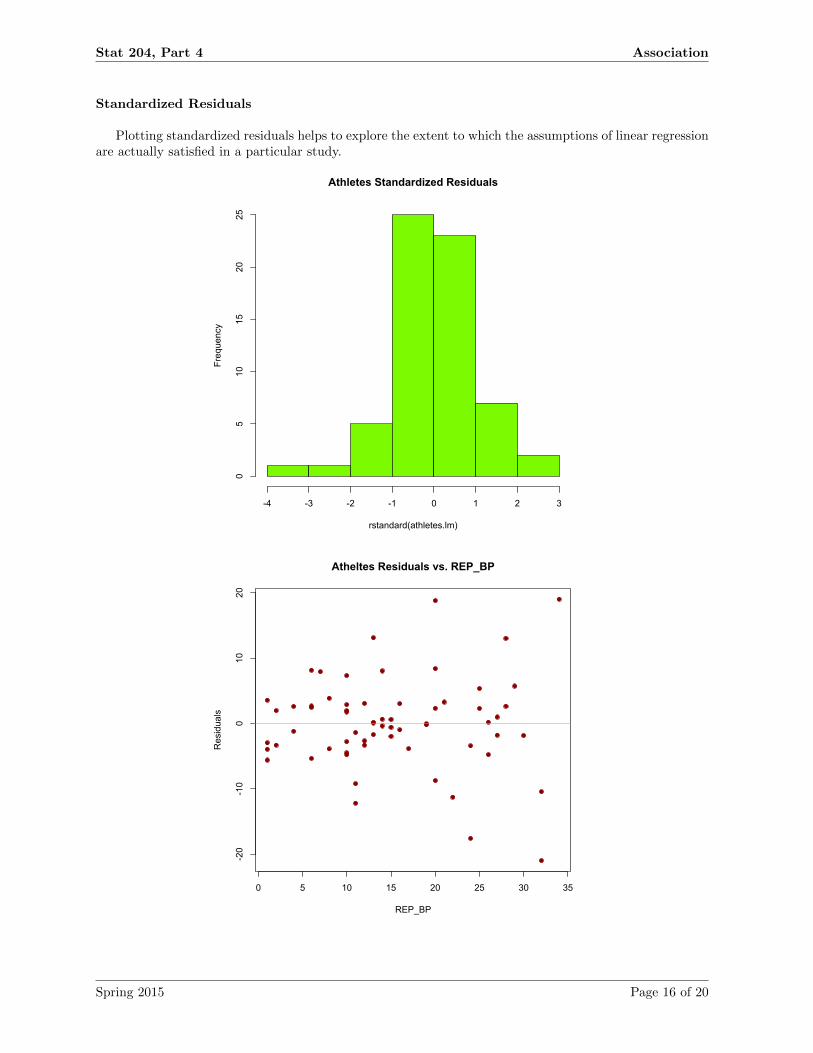
Standardized Residuals

Plotting standardized residuals helps to explore the extent to which the assumptions of linear regressionare actually satisfied in a particular study.

Athletes Standardized Residuals

rstandard(athletes.lm)

Frequency

-4 -3 -2 -1 0 1 2 3

05

1015

2025

0 5 10 15 20 25 30 35

-20

-10

010

20

Atheltes Residuals vs. REP_BP

REP_BP

Residuals

Spring 2015 of 20


House price standardized residuals

rstandard(houses.lm)

Frequency

-4 -2 0 2 4

020

4060

80

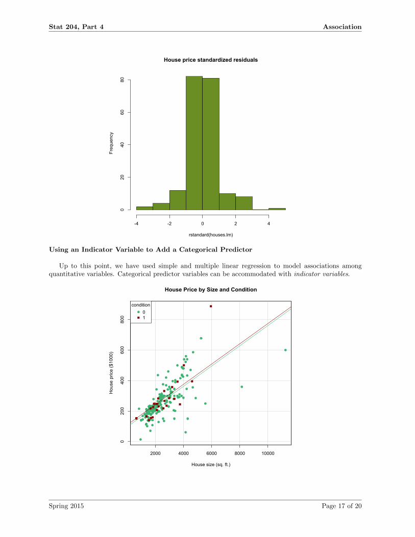
Using an Indicator Variable to Add a Categorical Predictor

Up to this point, we have used simple and multiple linear regression to model associations amongquantitative variables. Categorical predictor variables can be accommodated with indicator variables.

2000 4000 6000 8000 10000

0200

400

600

800

House Price by Size and Condition

House size (sq. ft.)

Hou

se p

rice

($10

00)

condition01

Spring 2015 of 20


Simpson’s Paradox

Simpson’s paradox exhibits a reversal in the direction of association when a new variable is added tothe model.

20 30 40 50

4060

80100

120

140

160

Assembly Defects vs. Assembly Time

Time (hrs)

Ass

embl

y D

efec

ts p

er 1

00 c

ars

20 30 40 50

4060

80100

120

140

160

Assembly Defects vs. Assembly Time (lm)

Time (hrs)

Ass

embl

y D

efec

ts p

er 1

00 c

ars

Japanese01

Spring 2015 of 20


Interaction

The essence of a linear model is that it is linear, but the actual data may present a rather differentstructure. Interaction may be present. Here, the linear model would say that adding a garage to a housewould increase the house price by a constant amount, regardless of the size of the house (red line), but thedata indicate that adding a garage to a house changes its price in an altogether different way (orange line).

2000 4000 6000 8000 10000

0200

400

600

800

House Selling Prices in OR (lm)

House Size

Hou

se P

rice

($)

Garage01

2000 4000 6000 8000 10000

0200

400

600

800

House Selling Prices in OR (interaction)

House Size

Hou

se P

rice

($)

Garage01

Spring 2015 of 20


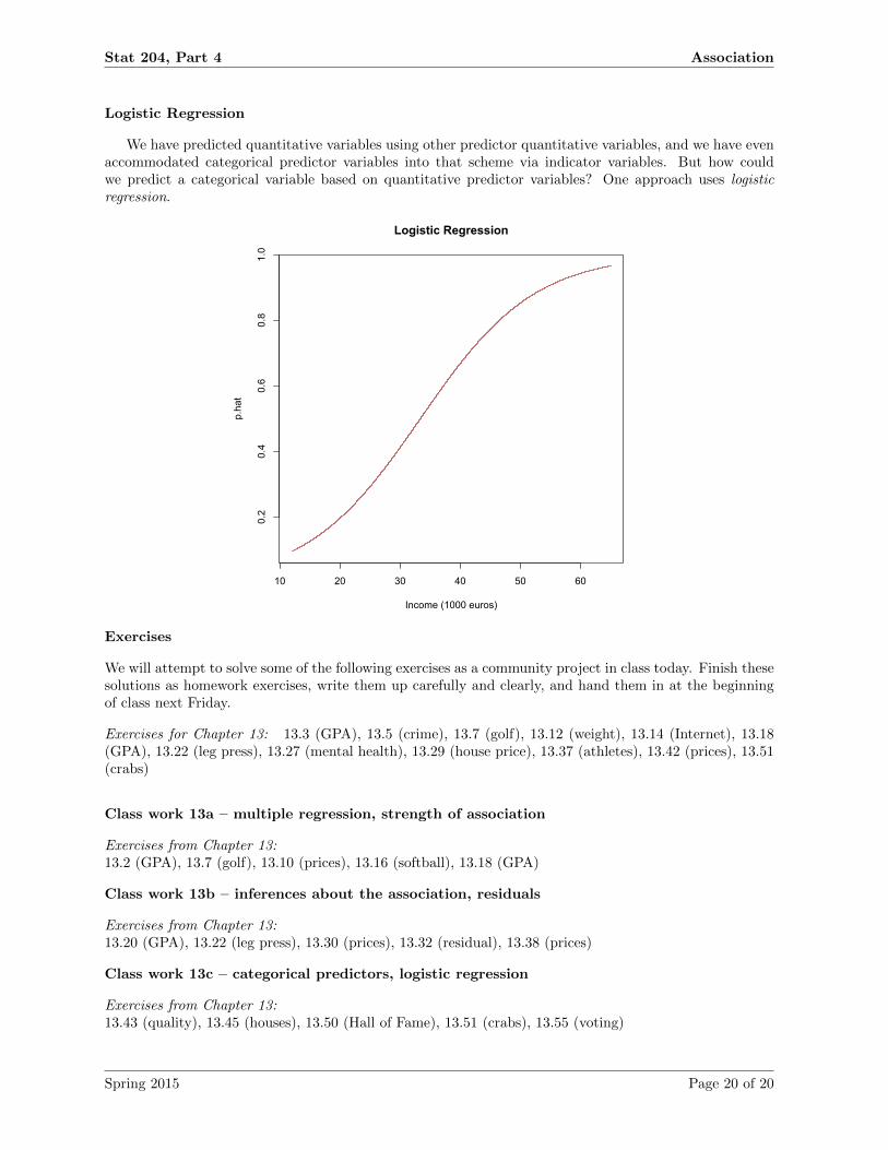
Logistic Regression

We have predicted quantitative variables using other predictor quantitative variables, and we have evenaccommodated categorical predictor variables into that scheme via indicator variables. But how couldwe predict a categorical variable based on quantitative predictor variables? One approach uses logisticregression.

10 20 30 40 50 60

0.2

0.4

0.6

0.8

1.0

Logistic Regression

Income (1000 euros)

p.hat

Exercises

We will attempt to solve some of the following exercises as a community project in class today. Finish thesesolutions as homework exercises, write them up carefully and clearly, and hand them in at the beginningof class next Friday.

Exercises for Chapter 13: 13.3 (GPA), 13.5 (crime), 13.7 (golf), 13.12 (weight), 13.14 (Internet), 13.18(GPA), 13.22 (leg press), 13.27 (mental health), 13.29 (house price), 13.37 (athletes), 13.42 (prices), 13.51(crabs)

Class work 13a – multiple regression, strength of association

Exercises from Chapter 13:13.2 (GPA), 13.7 (golf), 13.10 (prices), 13.16 (softball), 13.18 (GPA)

Class work 13b – inferences about the association, residuals

Exercises from Chapter 13:13.20 (GPA), 13.22 (leg press), 13.30 (prices), 13.32 (residual), 13.38 (prices)

Class work 13c – categorical predictors, logistic regression

Exercises from Chapter 13:13.43 (quality), 13.45 (houses), 13.50 (Hall of Fame), 13.51 (crabs), 13.55 (voting)

Spring 2015 of 20

chapter 13: multiple regressioncparrish.sewanee.edu/stat204 s2015/notes/part 04...

Documents