chapter 13, species diversity measureschapter 13 page 532 a biological community has an attribute...
TRANSCRIPT

CHAPTER 13
SPECIES DIVERSITY MEASURES (Version 5, 23 January 2014) Page
13.1 BACKGROUND PROBLEMS ........................................................................ 532
13.2 CONCEPTS OF SPECIES DIVERSITY ......................................................... 533
13.2.1 Species Richness ............................................................................. 534
13.2.2 Heterogeneity .................................................................................... 534
13.2.3 Evenness ........................................................................................... 535
13.3 SPECIES RICHNESS MEASURES ............................................................... 535
13.3.1 Rarefaction Method ........................................................................... 535
13.3.2 Jackknife Estimate ............................................................................ 547
13.3.3 Bootstrap Procedure ......................................................................... 551
13.3.4 Species Area Curve Estimates ........................................................ 553
13.4 HETEROGENEITY MEASURES .................................................................... 554
13.4.1 Logarithmic Series ............................................................................ 555
13.4.2 Lognormal Distribution ..................................................................... 564
13.4.3 Simpson's Index ................................................................................ 576
13.4.4 Shannon-Wiener Function ................................................................ 578
12.4.5 Brillouin’s Index ................................................................................ 583
13.5 EVENNESS MEASURES ............................................................................... 584
13.5.1 Simpson’s Measure of Evenness .................................................... 585
13.5.2 Camargo’s Index of Evenness ......................................................... 586
13.5.3 Smith and Wilson’s Index of Evenness .......................................... 586
13.5.4 Modified Nee Index of Evenness ..................................................... 587
13.6 BETA-DIVERSITY MEASUREMENTS ........................................................... 588
13.7 RECOMMENDATIONS .................................................................................. 590
13.8 SUMMARY ..................................................................................................... 591
SELECTED REFERENCES ................................................................................... 592
QUESTIONS AND PROBLEMS ............................................................................. 593

Chapter 13 Page 532
A biological community has an attribute which we can call species diversity, and
many different ways have been suggested for measuring this concept. Recent
interest in conservation biology has generated a strong focus on how to measure
biodiversity in plant and animal communities. Different authors have used different
indices to measure species diversity and the whole subject area has become
confused with poor terminology and an array of possible measures. Chiarucci (2012)
and Magurran and McGill (2011) have reviewed the problem. The problem at
present is that we have a diversity of measures for communities but they do not
always perform well (Xu et al. 2012). In this chapter we explore the measures that
are available for estimating the diversity of a biological community, and focus on
which measures are best to use for conservation assessment.
It is important to note that biodiversity has a broader meaning than species
diversity because it includes both genetic diversity and ecosystem diversity.
Nevertheless species diversity is a large part of the focus of biodiversity at the local
and regional scale, and we will concentrate here on how to measure species
diversity. The principles can be applied to any unit of ecological organization.
13.1 BACKGROUND PROBLEMS There are a whole series of background assumptions that one must make in order to
measure species diversity for a community. Ecologists tend to ignore most of these
difficulties but this is untenable if we are to achieve a coherent theory of diversity.
The first assumption is that the subject matter is well defined. Measurement of
diversity first of all requires a clear taxonomic classification of the subject matter. In
most cases ecologists worry about species diversity but there is no reason why
generic diversity or subspecific diversity could not be analyzed as well. Within the
classification system, all the individuals assigned to a particular class are assumed
to be identical. This can cause problems. For example, males may be smaller in size
than females – should they be grouped together or kept as two groups? Should
larval stages count the same as an adult stage? This sort of variation is usually
ignored in species diversity studies.

Chapter 13 Page 533
Most measures of diversity assume that the classes (species) are all equally
different. There seems to be no easy away around this limitation. In an ecological
sense sibling species may be very similar functionally while more distantly related
species may play other functional roles. Measures of diversity can address these
kinds of functional differences among species only if species are grouped into
functional groups (Boulangeat et al. 2012) or trophic nodes (De Visser et al. 2011).
Diversity measures require an estimate of species importance in the
community. The simple choices are numbers, biomass, cover, or productivity. The
decision in part will depend on the question being asked, and as in all questions
about methods in ecology you should begin by asking yourself what the problem is
and what hypotheses you are trying to test. Numbers are used by animal ecologists
in many cases as a measure of species importance, plant ecologists may use
biomass or cover, and limnologists may use productivity.
A related question is how much of the community should we include in our
sampling. We must define precisely the collection of species we are trying to
describe. Most authors pick one segment − bird species diversity or tree species
diversity and in doing so ignore soil nematode diversity and bacterial diversity.
Rarely do diversity measures cross trophic levels and only rarely are they applied to
whole communities. Colwell (1979) argues convincingly that ecologists should
concentrate their analyses on parts of the community that are functionally
interacting, the guilds of Root (1973). These guilds often cross trophic levels and
include taxonomically unrelated species in them. The choice of what to include in a
"community" is critical to achieving ecological understanding, yet there are no rules
available to help you make this decision. The functionally interacting networks can
be determined only by detailed natural history studies of the species in a community
(Baskerville et al. 2011).
13.2 CONCEPTS OF SPECIES DIVERSITY Early naturalists very quickly observed that tropical areas contained more species of
plants and animals than did temperate areas. To describe and compare different
communities, ecologists broke the idea of diversity down into three components –

Chapter 13 Page 534
alpha, beta, and gamma diversity. Alpha (α) diversity is local diversity, the diversity
of a forest stand, a grassland, or a stream. At the other extreme is gamma (γ)
diversity, the total regional diversity of a large area that contains several
communities, such as the eastern deciduous forests of the USA or the streams that
drain into the Missouri River. Beta (β) diversity is a measure of how different
community samples are in an area or along a gradient like from the headwaters of a
stream to its mouth, or from the bottom of a mountain to the top. Beta diversity links
alpha and gamma diversity, or local and regional diversity (Whittaker 1972). The
methods of estimating alpha and gamma diversity are fairly straightforward, but the
measurement of beta-diversity has been controversial (Ellison 2010).
We will proceed first to discuss methods that can be used to estimate alpha or
gamma diversity, and discuss beta-diversity later in this chapter. As ecological ideas
about diversity matured and ideas of quantitative measurement were introduced, it
became clear that the idea of species diversity contains two quite distinct concepts.
13.2.1 Species Richness This is the oldest and the simplest concept of species diversity - the number of
species in the community or the region. McIntosh (1967) coined the name species
richness to describe this concept. The basic measurement problem is that it is often
not possible to enumerate all of the species in a natural community or region,
particularly if one is dealing with insect communities or tropical plant assemblages. .
13.2.2 Heterogeneity If a community has 10 equally abundant species, should it have the same diversity
as another community with 10 species, one of which comprises 99% of the total
individuals? No, answered Simpson (1949) who proposed a second concept of
diversity which combines two separate ideas, species richness and evenness. In a
forest with 10 equally abundant tree species, two trees picked at random are likely to
be different species. But in a forest with 10 species, one of which is dominant and
contains 99% of all the individuals, two trees picked at random are unlikely to be
different species. Figure 12.1 illustrates this concept.

Chapter 13 Page 535
The term heterogeneity was first applied to this concept by Good (1953) and for
many ecologists this concept is synonymous with diversity (Hurlbert 1971). The
popularity of the heterogeneity concept in ecology is partly because it is relatively
easily measured.
13.2.3 Evenness Since heterogeneity contains two separate ideas − species richness and evenness −
it was only natural to try to measure the evenness component separately. Lloyd and
Ghelardi (1964) were the first to suggest this concept. For many decades field
ecologists had known that most communities of plants and animals contain a few
dominant species and many species that are relatively uncommon. Evenness
measures attempt to quantify this unequal representation against a hypothetical
community in which all species are equally common. Figure 13.1 illustrates this idea.
13.3 SPECIES RICHNESS MEASURES Some communities are simple enough to permit a complete count of the
number of species present, and this is the oldest and simplest measure of species
richness. Complete counts can often be done on bird communities in small habitat
blocks, mammal communities, and often for temperate and polar communities of
higher plants, reptiles, amphibians and fish. But it is often impossible to enumerate
every species in communities of insects, intertidal invertebrates, soil invertebrates,
or tropical plants, fish, or amphibians. How can we measure species richness when
we only have a sample of the community's total richness? Three approaches have
been used in an attempt to solve this sampling problem.
13.3.1 Rarefaction Method Species accumulation curves are a convenient way of expressing the principle
that as you sample more and more in a community, you accumulate more and more
species. Figure 13.2 illustrates this for small lizards sampled in Western Australia.
There are two directions one can go with a species accumulation curve. If you can fit
a statistical curve to the data, you can estimate the number of species you would
probably have found with a smaller sample size. Thus if you have collected 1650
lizards and you wish to compare species richness with another set of samples of
1000 lizards, you can use rarefaction to achieve an estimated number of species

Chapter 13 Page 536
that would be seen at a lower sampling rate. The second use is to extrapolate the
species accumulation curve to an asymptote that will reveal the total number of
species in the community.
No. of quadrats sampled0 2 4 6 8 10
No. o
f spe
cies
obse
rved
012345678
Community B
Community A
Species richness
0.0
0.2
0.4
Rela
tive
abun
danc
e
0.0
0.2
0.4
0.0
0.2
0.4
0.0
0.1
0.2
Species
Rela
tive
abun
danc
e
0.0
0.1
0.2
(a)
(b)
Community A
Community B
Community C
Heterogeneity
(c)
Evenness lower
Evenness higher
Evenness
1 3 5 7 9

Chapter 13 Page 537
Figure 13.1 Concepts of species diversity. (a) Species richness: community A has more species than community B and thus higher species richness. (b) Heterogeneity: community A has the same number of species as community B but the relative abundances are more even, so by a heterogeneity measure A is more diverse than B. Community C has the same abundance pattern as B but has more species, so it is more diverse than B. (c) Evenness: when all species have equal abundances in the community, evenness is maximal.
Figure 13.2 Species accumulation curve for the small reptiles of the Great Victoria Desert of Western Australia from Thompson et al. (2003). There were 1650 individuals of 31 species captured in pitfall traps. These curves illustrate the principle that the larger the sample size of individuals, the more species we expect to enumerate.
The problem with this second objective is that if there are many species in the
community, species accumulation curves keep rising and there is much uncertainty
about when they might level off at maximum species richness. Let us deal with the
first objective.
One problem that frequently arises in comparing community samples is that
they are based on different samples sizes. The larger the sample, the greater the
expected number of species. If we observe one community with 125 species in a
collection of 2200 individuals and a second community with 75 species in a
collection of 750 individuals we do not know immediately which community has
higher species richness. One way to overcome this problem is to standardize all
No. of individuals caught0 250 500 750 1000 1250 1500 1750 2000
Accu
mul
ated
num
ber o
f spe
cies
0
5
10
15
20
25
30
35

Chapter 13 Page 538
samples from different communities to a common sample size of the same number
of individuals. Sanders (1968) proposed the rarefaction method for achieving this
goal. Rarefaction is a statistical method for estimating the number of species
expected in a random sample of individuals taken from a collection. Rarefaction
answers this question: if the sample had consisted of n individuals (n<N), what
number of species (s) would likely have been seen? Note that if the total sample has
S species and N individuals, the rarefied sample must always have n < N and s < S
(see Figure 13.3).
Sanders' (1968) original rarefaction algorithm was wrong, and it was corrected
independently by Hurlbert (1971) and Simberloff (1972) as follows:
( )1
ˆ 1 i
s
ni
N Nn
E SNn
=
− = −
∑ (13.1)
where:
( )ˆ Expected number of species in a random sample of individuals Total number of species in the entire collection Number of individuals in species
Total number of individuals in collecti
n
i
E S nS
N iN
==== on
Value of sample size (number of individuals) chosen for standardization ( )
Number of combinations of individuals that can be chosen from
a set of individuals
iNn
n NN nn
N
==
≤ =
=
∑
( )!/ ! !N n N n−
The large-sample variance of this estimate was given by Heck et al. (1975) as:
( )1
1
1
1 1
1
ˆvar
2
is
i
i
ni
s si J
i j i
N NnN N
n NnNS N Nn N N i
n nN N Nn N
n
=−
−
= = +
− − − + = − − − − −
∑
∑ ∑
(13.2)

Chapter 13 Page 539
where
( )ˆvar Variance of the expected number of species in a random sample of individuals
nSn
=
and all other terms are defined above.
Figure 13.3 Rarefaction curve for the diatom community data from Patrick (1968). There were 4874 individuals in 112 species in this sample (“Box 8”). Original data in Table 13.1. If a sample of 2000 individuals were taken, we would expect to find only 94 species, for example. This illustrates the general principle that the larger the sample size of individuals, the more species we expect to enumerate.
TABLE 13.1 TWO SAMPLES OF A DIATOM COMMUNITY OF A SMALL CREEK IN PENNSYLVANIA IN 1965a
Number of individuals
Number of individuals
Species Box 8 Box 7 Species Box 8 Box 7 Nitzxchia frustulum v. perminuta 1446 1570 Melosira italica v. valida 6 15
Synedra parasitica v. subconstricta 456 455 Navicula cryptoocephala v. veneta 6 6
Navicula cryptocephala 450 455 Cymbella turgida 5 8
Cyclotella stelligera 330 295 Fragilaria intermedia 5 5
Navicula minima 318 305 Gomphonema augustatum v. obesa 5 16
No. of individuals in sample0 1000 2000 3000 4000
Expe
cted
num
ber o
f spe
cies
0
20
40
60
80
100
120
Diatoms in Box 8
N

Chapter 13 Page 540
N. secreta v. apiculata 306 206 G. angustatum v. producta 5 4
Nitzschia palea 270 225 G. ongiceps v. subclavata 5 9
N. frustulum 162 325 Meridion circulare 5 4
Navicula luzonensis 132 78 Melosira ambigua 5 --
Nitzschia frustulum v. indica 126 180 Nitzschia acicularis 5 --
Melosira varians 118 140 Synedra rumpens v. familiaris 5 37
Nitzschia amphibia 93 95 Cyclotella meneghiniana 4 8
Achnanthes lanceolata 75 275 Gyrosigma spencerii 4 2
Stephanodiscus hantzschii 74 59 Fragilaria construens v. venter 3 --
Navicula minima v. atomoides 69 245 Gomphonema gracile 3 10
N. viridula 68 72 Navicula cincta 3 2
Rhoicosphenia curvata v. minor 61 121 N. gracilis fo. Minor 3 --
Navicula minima v. atomoides 59 47 Navicula decussis 3 2
N. pelliculsa 54 19 N. pupula v. capitat 3 10
Melosira granulata v. angustissima 54 73 N. symmetrica 3 --
Navicula seminulum 52 36 Nitzxchia dissipata v. media 3 4
N. gregaria 40 34 N. tryblionella v. debilis 3 1
Nitzschia capitellata 40 16 N. sigmoidea 3 --
Achnanthes subhudsonis v. kraeuselii 39 51 Anomoeoneis exilis 2 --
A minutissima 35 61 Caloneis hyalina 2 2
Nitzschia diserta 35 53 Diatoma vulgare 2 --
Amphora ovalis v. pediculus 33 53 Eunotia pectinalis v. minor 2 1
Cymbella tumida 29 95 Fragilaria leptostauron 2 3
Synedra parasitica 24 42 Gomphonema constrictum 2 --
Cymbella ventricosa 21 27 G. intricatum v. pumila 2 10
Navicula paucivisitat 20 12 Navicula hungarica v. capitat 2 5
Nitzschia kutzingiana 19 70 N. protraccta 2 3
Gomphonema parvulum 18 66 Synedra acus v. angustissima 2 --
Rhoicosphenia curvata 18 22 Bacillaria paradoxa 1 --
Synedra ulna 18 36 Cyclotella kutzingiana 1 --
Surirella angustata 17 11 Cymbella triangulum 1 --
Synedra ulna v. danica 17 37 Cocconeis sp. 1 --
Navicula pupula 17 27 Caloneis bacillum 1 3
Achnanthes biporoma 16 32 Fragilaria bicapitat 1 --
Stephanodiscus astraea v. minutula 16 21 Frustulia vularis 1 --
Navicula germainii 13 19 Gomphonema carolinese 1 1
Denticula elegans 12 4 G. sp. 1 --
Gomphonema sphaerophorum 11 40 Navicula capitat v. hungarica 1 1
Synedra rumpens 11 13 N. contenta f. biceps 1 1
S. vaucheriae 11 14 N. cincta v. rostrata 1 --
Cocconeis placentula v. euglypta 10 5 N. americana 1 --
Navicula menisculus 10 5 Nitzschia hungarica 1 --

Chapter 13 Page 541
Nitzschia linearis 10 18 N. sinuata v. tabularia 1 --
Stephanoddiscus invisitatus 10 22 N. confinis 1 5
Amphora ovalis 9 16 Synedra pulchella v. lacerata 1 1
Cymbella sinuata 9 5 Surirella ovata 1 3
Gyrosigma wormleyii 9 5 Achnanthes cleveii -- 2
Nitzschia fonticola 9 6 Amphora submontana -- 1
N. bacata 9 7 Caloneis silicula v. ventricosa -- 3
Synedra rumpens v. meneghiniana 9 17 Eunotia lunaris -- 2
Cyclotella meneghiniana small 8 4 E. tenella -- 1
Nitzschia gracilis v. minor 8 10 Fragilaria pinnata -- 3
N. frustulum v. subsalina 7 10 Gyrosigma scalproides -- 1
N. subtilis 7 16 Gomphonema sparsistriata -- --
Cymbella affinis 6 3 Meridion circulara v. constricta -- 3
Cocconeis placetula v. lineata 6 13 Navicula tenera -- 3
N. omissa -- 1
N. ventralis -- 1
N. mutica -- 1
N. sp. -- 1
N. mutica v. cohnii -- 1
Nitzschia brevissima -- 1
N. frequens -- 1
a The numbers of individuals settling on glass slides were counted. Data from Patrick (1968).
Box 13.1 illustrates the calculation of the rarefaction method for some rodent
data. Because these calculations are so tedious, a computer program should
normally be used for the rarefaction method. Program DIVERSITY (Appendix 2 page
000) can do these calculations. It contains a modified version of the program given
by Simberloff (1978). The program EstimateS developed by Robert Colwell
(http://viceroy.eeb.uconn.edu/estimates/ ) calculates these estimates as well as
many others for species richness.
Box 13.1 CALCULATION OF EXPECTED NUMBER OF SPECIES BY THE RAREFACTION METHOD
A sample of Yukon rodents produced four species in a collection of 42 individuals. The species abundances were 21, 16, 3, and 2 individuals. We wish to calculate the expected species richness for samples of 30 individuals. Expected Number of Species From equation (13.1)

Chapter 13 Page 542
( )1
ˆ 1i
s
ni
N Nn
E SNn
=
− = −
∑
( )30
42 21 42 16 42 3 30 30 30ˆ 1 1 1
42 42 4230 30 30
42 2 30 1
4230
E S
− − − = − + − + −
− + −
42 21 21 0 (by definition) 30 30− = =
( )1042!42 1.1058 1030 30! 42 30 !
= = × −
42 16 26 0 (by definition) 30 30− = =
( )839!42 3 2.1192 10 30 30! 39 30 !
− = = × −
( )840!42 2 8.4766 10 30 30! 40 30 !
− = = × −
( )8 8
30 10 102.1192 10 8.4766 10ˆ 1 1 1 1 1.1058 10 1.1058 10
1 1 0.981 0.923 3.90 species
E S × ×
= + + − + − × × = + + +=
These calculations are for illustration only, since you would never use this method on such a small number of species. Large Sample Variance of the Expected Number of Species From equation (13.2)

Chapter 13 Page 543
( )1
1
1
1 1
1 +
ˆvar
2
is
i
i
ni
s si J
i j i
N NnN N
n NnNS N Nn N N i
n nN N Nn N
n
=−
−
= = +
− − − = − − − − −
∑
∑ ∑
( )1
30
21 26 3930 30 3021 26 391 1 1 30 30 3042 42 4230 30 30403040 1 30 4230
42ˆvar = 30S−
− + − + −
+ −
42 21 42 16 30 3042 21 162 30 42
3042 21 42 3 30 3042 21 3 30 42
30
42 21 3+
− − − − + −
− − − − + −
− −42 21 42 2 30 30 30 42
3042 16 42 3 30 3042 16 3 30 42
3042 16 42 2 30 342 16 2 - 30
− − −
− − − − + −
− − − − +
0
4230
42 3 42 2 30 3042 3 2 30 42
30
− −
− − + − Note that for this particular example almost all of the terms are zero.
Chapter 13 Page 544
( ) ( ) ( )( )8 8
-10630
2.0785 10 7.8268 10ˆvar 1.1058 10 2 5.9499 10 0.0885
S × + ×
= × + − × =
( ) ( )30 30ˆ ˆStandard deviation of var
0.0885 0.297
S S=
= =
These tedious calculations can be done by Program DIVERSITY (see Appendix 2, page 000) or by Program EstimateS from Colwell et al.(2012).
There are important ecological restrictions on the use of the rarefaction
method. Since rarefaction is not concerned with species names, the communities to
be compared by rarefaction should be taxonomically similar. As Simberloff (1979)
points out, if community A has the larger sample primarily of butterflies and
community B has the smaller sample mostly of moths, no calculations are necessary
to tell you that the smaller sample is not a random sample of the larger set.
Sampling methods must also be similar for two samples to be compared by
rarefaction (Sanders 1968). For example, you should not compare insect light trap
samples with insect sweep net samples, since whole groups of species are
amenable to capture in one technique but not available to the other. Most sampling
techniques are species-selective and it is important to standardize collection
methods.
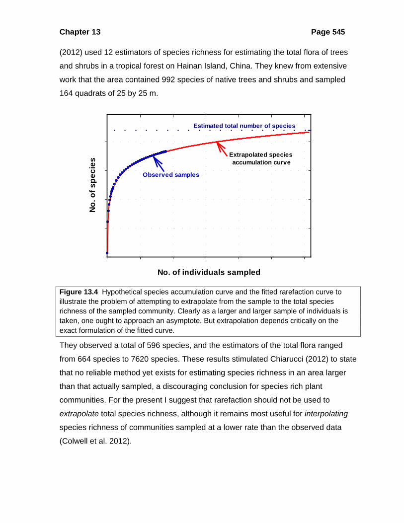
The second objective is both more interesting and more difficult. If the species
accumulation curve does plateau, we should be able to determine the complete
species richness of the fauna or flora by extrapolating the rarefaction curve (Figure
13.4). But the only way one can extrapolate beyond the limits of the samples is by
assuming an underlying statistical distribution.
The perils of attempting to extrapolate have been discussed by many
ecologists. For example, Thompson et al. (2003) fitted 11 non-linear regression
models to lizard data from Western Australia and concluded that different regression
models fitted data from different sites and that extensive sampling was required to
obtain even an approximate estimate of total species numbers in an area. Xu et al.
Chapter 13 Page 545
(2012) used 12 estimators of species richness for estimating the total flora of trees
and shrubs in a tropical forest on Hainan Island, China. They knew from extensive
work that the area contained 992 species of native trees and shrubs and sampled
164 quadrats of 25 by 25 m.
Figure 13.4 Hypothetical species accumulation curve and the fitted rarefaction curve to illustrate the problem of attempting to extrapolate from the sample to the total species richness of the sampled community. Clearly as a larger and larger sample of individuals is taken, one ought to approach an asymptote. But extrapolation depends critically on the exact formulation of the fitted curve.
They observed a total of 596 species, and the estimators of the total flora ranged
from 664 species to 7620 species. These results stimulated Chiarucci (2012) to state
that no reliable method yet exists for estimating species richness in an area larger
than that actually sampled, a discouraging conclusion for species rich plant
communities. For the present I suggest that rarefaction should not be used to
extrapolate total species richness, although it remains most useful for interpolating
species richness of communities sampled at a lower rate than the observed data
(Colwell et al. 2012).
No. of individuals sampled
No. o
f spe
cies
Estimated total number of species
Extrapolated species accumulation curve
Observed samples
Chapter 13 Page 546
One assumption that rarefaction does make is that all individuals in the
community are randomly dispersed with respect to other individuals of their own or
of different species. In practice most distributions are clumped (see Chapter 4) within
a species and there may be positive or negative association between species. Fager
(1972) used computer simulations to investigate what effect clumping would have on
the rarefaction estimates, and observed that the more clumped the populations are,
the greater the overestimation of the number of species by the rarefaction method.
The only way to reduce this bias in practice is to use large samples spread widely
throughout the community being analyzed.
The variance of the expected number of species (equation 13.2) is appropriate
only with reference to the sample under consideration. If you wish to ask a related
question: given a sample of N individuals from a community, how many species
would you expect to find in a second, independent sample of n (n < N) individuals?
Smith and Grassle (1977) give the variance estimate appropriate for this more
general question, and have a computer program for generating these variances.
Simberloff (1979) showed that the variance given in equation (13.2) provides
estimates only slightly smaller than the Smith and Grassle (1977) estimator.
Figure 13.3 illustrates a rarefaction curve for the diatom community data in
Table 13.1. James and Rathbun (1981) provide additional examples from bird
communities.
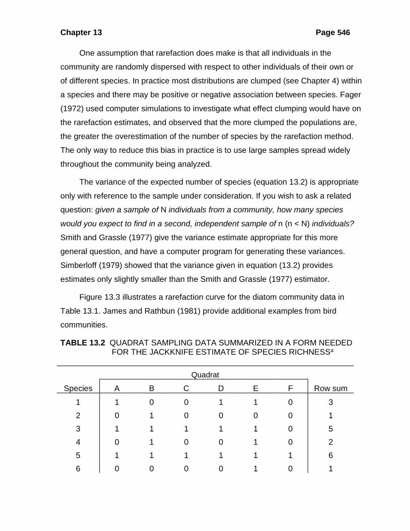
TABLE 13.2 QUADRAT SAMPLING DATA SUMMARIZED IN A FORM NEEDED FOR THE JACKKNIFE ESTIMATE OF SPECIES RICHNESSa
Quadrat
Species A B C D E F Row sum
1 1 0 0 1 1 0 3 2 0 1 0 0 0 0 1 3 1 1 1 1 1 0 5 4 0 1 0 0 1 0 2 5 1 1 1 1 1 1 6 6 0 0 0 0 1 0 1

Chapter 13 Page 547
7 0 0 1 1 1 1 4 8 1 1 0 0 1 1 4
a Only presence-absence data are required. Unique species are those whose row sums are 1 (species 2 and 6 in this example). 0 = absent; 1 = present.
13.3.2 Jackknife Estimate When quadrat sampling is used to sample the community, it is possible to use a
variety of nonparametric approaches. They have been reviewed comprehensively by
Magurran (2004) and I present only one here, the jackknife*, a non-parametric
estimator of species richness. This estimate, called ‘Jackknife 1 by Magurran (2004),
is based on the observed frequency of rare species in the community, and is
obtained as follows (Heltshe and Forrester 1983a). Data from a series of random
quadrats are tabulated in the form shown in Table 13.2, recording only the presence
(1) or absence (0) of the species in each quadrat. Tally the number of unique
species in the quadrats sampled. A unique species is defined as a species that
occurs in one and only one quadrat. Unique species are spatially rare species and
are not necessarily numerically rare, since they could be highly clumped. From
Heltshe and Forrester (1983a) the jackknife estimate of the number of species is:
1ˆ nS s kn− = +
(13.3)
where: ˆ Jackknife estimate of species richness Observed total number of species present in quadrats Total number of quadrats sampled Number of unique species
Ss nnk
====
The variance of this jackknife estimate of species richness is given by:
( ) ( )2
2
1
1ˆvar s
Jj
n kS j fn n=
− = −
∑ (13.4)
where:
* For a general discussion of jackknife estimates, see Chapter 16, page 000.
Chapter 13 Page 548
( )ˆvar Variance of jackknife estimate of species richness Number of quadrats containing unique species ( 1, 2, 3, . ) Number of unique species Total number of quadrats sampled
J
Sf j j skn
== ===
This variance can be used to obtain confidence limits for the jackknife estimator:
( )ˆ ˆvarS t Sα± (13.5)
where:
( )
ˆ Jackknife estimator of species richness (equation 12.3) Student's value for 1 degrees of freedom
for the appropriate value of ˆ ˆvar Variance of from equation (12.4)
St t n
S S
α
α
== −
=
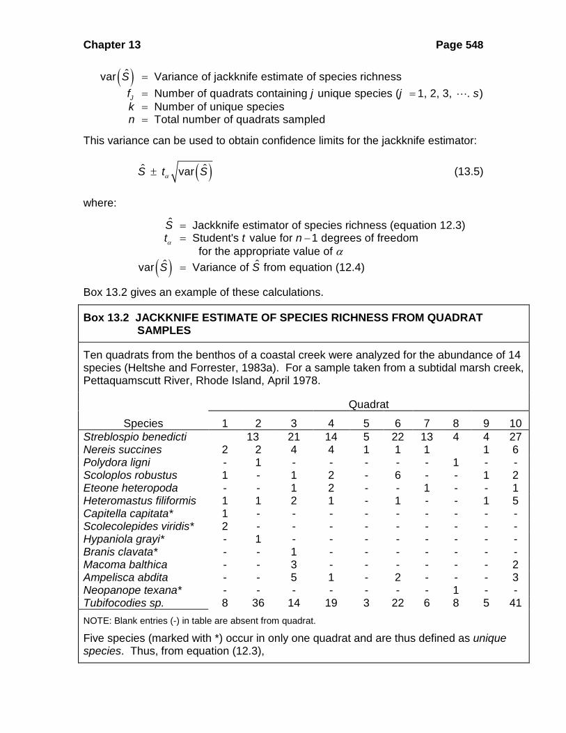
Box 13.2 gives an example of these calculations.
Box 13.2 JACKKNIFE ESTIMATE OF SPECIES RICHNESS FROM QUADRAT SAMPLES
Ten quadrats from the benthos of a coastal creek were analyzed for the abundance of 14 species (Heltshe and Forrester, 1983a). For a sample taken from a subtidal marsh creek, Pettaquamscutt River, Rhode Island, April 1978.
Quadrat
Species 1 2 3 4 5 6 7 8 9 10 Streblospio benedicti 13 21 14 5 22 13 4 4 27 Nereis succines 2 2 4 4 1 1 1 1 6 Polydora ligni - 1 - - - - - 1 - - Scoloplos robustus 1 - 1 2 - 6 - - 1 2 Eteone heteropoda - - 1 2 - - 1 - - 1 Heteromastus filiformis 1 1 2 1 - 1 - - 1 5 Capitella capitata* 1 - - - - - - - - - Scolecolepides viridis* 2 - - - - - - - - - Hypaniola grayi* - 1 - - - - - - - - Branis clavata* - - 1 - - - - - - - Macoma balthica - - 3 - - - - - - 2 Ampelisca abdita - - 5 1 - 2 - - - 3 Neopanope texana* - - - - - - - 1 - - Tubifocodies sp. 8 36 14 19 3 22 6 8 5 41 NOTE: Blank entries (-) in table are absent from quadrat.
Five species (marked with *) occur in only one quadrat and are thus defined as unique species. Thus, from equation (12.3),

Chapter 13 Page 549
( )
1ˆ
9ˆ 14 510
18.5 species
nS s kn
S
− = + = +
=
The variance, from equation (12.4), is
( ) ( )2
2
1
1ˆvar s
Jj
n kS j fn n=
− = −
∑
From the table we tally:
No. of unique spp., j
No. of quadrats containing j unique species, fJ
1 3 (i.e., quadrats 2,3,and 8) 2 1 (i.e., quadrat 1) 3 0 4 0 5 0 Thus,
( ) ( ) ( ) ( )2
2 29 5ˆvar 1 3 2 1 10 10
4.05
S = + −
=
For this small sample, for 95% confidence tα = 2.26, and thus the 95% confidence interval would be approximately
( )( )18.5 2.26 4.05±
or 14 to 23 species. Program DIVERSITY (Appendix 2, page 000), can do these calculations for quadrat data.
There is some disagreement about the relative bias of the jackknife estimator
of species richness tends to be biased. Heltshe and Forrester (1983a) state that it
has a positive bias, that is, it tends to overestimate the number of species in a
community. Palmer (1990) found that the jackknife estimator had a slight negative
Chapter 13 Page 550
bias in his data. This bias was much less than the negative bias of the observed
number of species (S).
Note from equation (13.3) that the maximum value of the jackknife estimate of
species richness is twice the observed number of species. Thus this approach
cannot be used on communities with exceptionally large numbers of rare species, or
on communities that have been sampled too little (so S is less than half the species
present).
Two other non-parametric estimators of species richness for
presence/absence data were developed by A. Chao and are called ‘Chao 1’ and
‘Chao 2’ in the literature (Colwell and Coddington 1994). They are very similar in
concept. Chao 1 is based on presence/absence quadrat data and is given by:
( )( )
1 11
2
1)ˆ2 1Chao obs
f fS S
f−
= + +
(13.6)
where
1
1
2
ˆ bias corrected Chao 1 species richness estimator number of species observed in total number of species represented only once in the samples (unique species) number of species repre
Chao
obs
SS
ff
==== sented only twice in the samples
The variance of the Chao 1 estimator is given by:
( ) ( )( )
( )( )
( )( )
2 221 1 1 1 1 2 1
1 2 42 2 2
1 1 1ˆˆvar2 1 4 1 4 1Chao
f f f f f f fS
f f f
− − −= + +
+ + + (13.7)
where f1 and f2 are defined above.
Chao 2 is based on counts of individuals in quadrats or samples and is given by:
( )
( )1 1
22
1 1ˆ
2 1Chao obs
t Q QtS S
Q
− − = + +
(13.8)
where
2
1
2
ˆ bias corrected Chao 2 estimator of species richness number of quadrats or samples number of species that occur in one sample only number of species that occur in two samples only
ChaoSt
====
Chapter 13 Page 551
The variance of the Chao 2 estimator is given by:
( ) ( )( )
( )( )
( )( )
2 22 2 21 1 1 1 1 2 1
2 2 42 2 2
1 2 1 11 1 1ˆˆvar2 1 4 1 4 1Chao
Q Q Q Q Q Q Qm m mSm Q m mQ Q
− − −− − − = + + + + + (13.9)
Confidence limits for the two Chao estimators are given by using these variances in
this equation:
Lower 95% confidence limit
Upper 95% confidence limit obs
obs
TSK
S TK
= +
= + (13.10)
where
( )2
ˆvarexp 1.96 log 1
obs
Chaoe
T Chao S
SK
T
= − = +
and Chao may be either of the estimators, Chao 1 or Chao 2.
Chao’s estimators provide minimum estimates of species richness and are
meant to be applied to a single community rather than a gradient of communities. In
the data tested by Xu et al. (2012) the Chao 1 estimator was 68% of the true value
and Chao 2 was 79% of the true value. Chao and Shin (2010) present many other
non-parametric estimators of species richness that are computed in Program
SPADE.
13.3.3 Bootstrap Procedure One alternative method of estimating species richness from quadrat samples is to
use the bootstrap procedure (Smith and van Belle 1984). The bootstrap method* is
related to the jackknife but it requires simulation on a computer to obtain estimates.
The essence of the bootstrap procedure is as follows: given a set of data of species
presence/absence in a series of q quadrats (like Table 13.2):
* See Chapter 16, page 000 for more discussion of the bootstrap method.

Chapter 13 Page 552
1. Draw a random sample of size n from the q quadrats within the computer, using
sampling with replacement; this is the "bootstrap sample"
2. Calculate the estimate of species richness from the equation (Smith and van Belle
1984):
( ) ( )ˆ 1 niB S S p= + −∑ (13.11)
where:
( )ˆ = Bootstrap estimate of species richness = Observed number of species in original data = Proportion of the bootstrap quadrats that have species presenti
B SSp n i
3. Repeat steps (a) and (b) N times in the computer, where N is between 100 and
500.
The variance of this bootstrap estimate is given by:
( ) ( ) ( )
( ) ( ){ }i
ˆvar 1 1 1
1 1
n ni i
nnnij i j
j i j
B S p p
q p p≠
= − − − + − − − −
∑
∑∑ (13.12)
where:
( )ˆvar Variance of the bootstrap estimate of species richness, , As defined above
Proportion of the bootstrap quadrats that have both species and species absent
i j
ij
B Sn p p
q ni j
= ==
Smith and van Belle (1984) recommend the jackknife estimator when the number of
quadrats is small and the bootstrap estimator when the number of quadrats is large.
The empirical meaning of “small” and “large” for natural communities remains
unclear; perhaps n = 100 quadrats is an approximate division for many community
samples, but at present this is little more than a guess. For Palmer’s data (1990)
with n = 40 quadrats the bootstrap estimator had twice the amount of negative bias
as did the jackknife estimator. Both the bootstrap and the jackknife estimators are
limited to maximum values twice the number of observed species, so they cannot be
Chapter 13 Page 553
used on sparsely sampled communities. In the test of Xu et al. (2012) the bootstrap
estimator was 67% of the true value of species richness.
13.3.4 Species Area Curve Estimates One additional way of estimating species richness is to extrapolate the species area
curve for the community. Since the number of species tends to rise with the area
sampled, one can fit a regression line and use it to predict the number of species on
a plot of any particular size. This method is useful only for communities which have
enough data to compute a species-area curve, and so it could not be used on
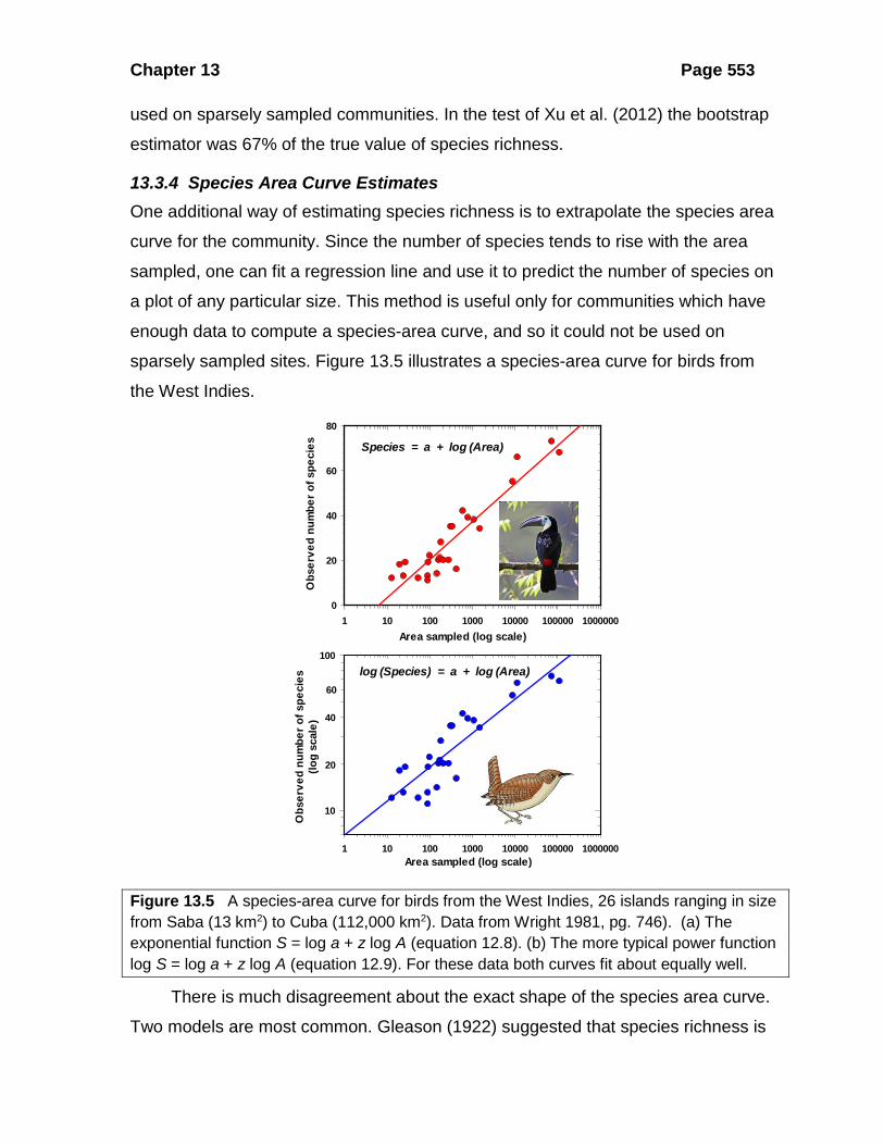
sparsely sampled sites. Figure 13.5 illustrates a species-area curve for birds from
the West Indies.
Figure 13.5 A species-area curve for birds from the West Indies, 26 islands ranging in size from Saba (13 km2) to Cuba (112,000 km2). Data from Wright 1981, pg. 746). (a) The exponential function S = log a + z log A (equation 12.8). (b) The more typical power function log S = log a + z log A (equation 12.9). For these data both curves fit about equally well.
There is much disagreement about the exact shape of the species area curve.
Two models are most common. Gleason (1922) suggested that species richness is
Area sampled (log scale)1 10 100 1000 10000 100000 1000000
Obs
erve
d nu
mbe
r of s
peci
es
0
20
40
60
80
Area sampled (log scale)1 10 100 1000 10000 100000 1000000
Obs
erve
d nu
mbe
r of s
peci
es(lo
g sc
ale)
10
100
Species = a + log (Area)
log (Species) = a + log (Area)
20
40
60

Chapter 13 Page 554
proportional to the logarithm of the area sampled, so that one should compute a
semi-log regression of the form:
log( )S a A= + (13.13)
where
Number of species ( species richness)Area sampledy-intercept of the regression
SAa
= ===
Preston (1962) argued that the species area curve is a log-log relationship of the
form:
log( ) log( )S a A= + (13.14)
where all terms are defined above. Palmer (1990) found that both these regressions
overestimated species richness in his samples, and that the log-log regression
(equation 13.14) was a particularly poor estimator. The semi-log form of the species-
area regression was highly correlated with species richness, in spite of its bias, and
thus could serve as an index of species richness.
The value of all area-based estimators of species richness is that they should
allow you to extrapolate data from a local area to a much larger region. For example,
Harte et al. (2009) used tree data from small plots of 0.25 ha (average 32 species
per plot) to estimate the tree species of a region of 60,000 km2 in India by means of
a species-area model (estimated total of 1070 species). Xu et al. (2012) found that
all the area-based estimators of species richness greatly overestimated the number
of species in a tropical rain forest.
At present I can suggest that any estimator of species richness should be
treated as an index of species richness rather than an accurate estimate of total
species richness for a larger area. No reliable method has yet been developed to
predict the species richness of an ecosystem that is much larger than the actual
area sampled (Chiarucci 2012).
13.4 HETEROGENEITY MEASURES The measurement of diversity by means of heterogeneity indices has proceeded
along two relatively distinct paths. The first approach is to use statistical sampling
Chapter 13 Page 555
theory to investigate how communities are structured. The logarithmic series was
first applied by Fisher, Corbet, and Williams (1943) to a variety of community
samples. Preston (1948, 1962) applied the lognormal distribution to community
samples. Because of the empirical nature of these statistical distributions, other
workers looked to information theory for appropriate measures of diversity.
Arguments continue about the utility of both of these approaches since they are not
theoretically justified (Washington 1984, Hughes 1986, Magurran 2004, Magurran
and McGill 2011). But both approaches are widely used in diversity studies and it
would be premature to dismiss any measure because it lacks comprehensive
theoretical justification, since a diversity measure could be used as an index to
diversity for practical studies.
It is important to keep in mind the ecological problem for which we wish to use
these measures of heterogeneity. What is the hypothesis you wish to investigate
using a heterogeneity measure? The key is to obtain some measure of community
organization related to your hypothesis of how the relative abundances vary among
the different species in the community. Once we can measure community
organization we can begin to ask questions about patterns shown by different
communities and processes which can generate differences among communities.
13.4.1 Logarithmic Series One very characteristic feature of communities is that they contain comparatively
few species that are common and comparatively large numbers of species that are
rare. Since it is relatively easy to determine for any given area the number of species
on the area and the number of individuals in each of these species, a great deal of
information of this type has accumulated (Williams 1964). The first attempt to
analyze these data was made by Fisher, Corbet, and Williams (1943).
In many faunal samples the number of species represented by a single
specimen is very large; species represented by two specimens are less numerous,
and so on until only a few species are represented by many specimens. Fisher,
Corbet, and Williams (1943) plotted the data and found that they fit a "hollow curve"
(Figure 13.6). Fisher concluded that the data available were best fitted by the

Chapter 13 Page 556
logarithmic series, which is a series with a finite sum whose terms can be written as
a function of two parameters:
2 3 4
, , , ,2 3 4x x xx α α αα (13.15)
where:
2 = Number of species in the total catch represented by individual
= Number of species represented by two individuals, and so on2
x onexα
α
Figure 13.6 Relative abundance of Lepidoptera (butterflies and moths) captured in a light trap at Rothamsted, England, in 1935. Not all of the abundant species are shown. There were 37 species represented in the catch by only a single specimen (rare species); one very common species was represented by 1799 individuals in the catch (off the graph to the right!). A total of 6814 individuals were caught, representing 197 species. Six common species made up 50 percent of the total catch. (Source: Williams, 1964.)
The sum of the terms in the series is equal to ( ) log 1e xα− − which is the total
number of species in the catch. The logarithmic series for a set of data is fixed by
two variables, the number of species in the sample and the number of individuals in
the sample. The relationship between these is:
log 1eNS αα
= +
(13.16)
No. of individuals represented in sample
0 10 20 30 40
Num
ber o
f spe
cies
0
10
20
30
40
Common speciesRare species
.......
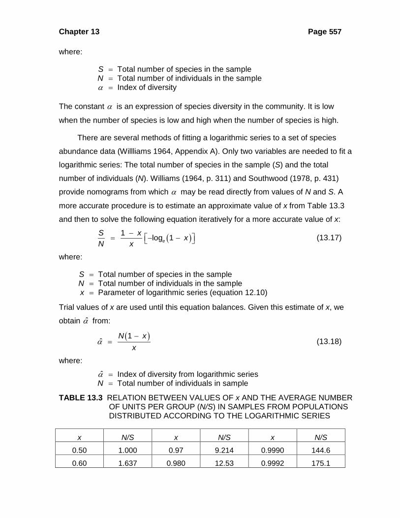
Chapter 13 Page 557
where:
Total number of species in the sample Total number of individuals in the sample Index of diversity
SNα
===
The constant α is an expression of species diversity in the community. It is low
when the number of species is low and high when the number of species is high.
There are several methods of fitting a logarithmic series to a set of species
abundance data (Willliams 1964, Appendix A). Only two variables are needed to fit a
logarithmic series: The total number of species in the sample (S) and the total
number of individuals (N). Williams (1964, p. 311) and Southwood (1978, p. 431)
provide nomograms from which α may be read directly from values of N and S. A
more accurate procedure is to estimate an approximate value of x from Table 13.3
and then to solve the following equation iteratively for a more accurate value of x:
( )1 log 1eS x xN x
− = − − (13.17)
where:
Total number of species in the sample Total number of individuals in the sample Parameter of logarithmic series (equation 12.10)
SNx
===
Trial values of x are used until this equation balances. Given this estimate of x, we
obtain α from:
( )1ˆ
N xx
α−
= (13.18)
where:
ˆ Index of diversity from logarithmic series Total number of individuals in sampleN
α ==
TABLE 13.3 RELATION BETWEEN VALUES OF x AND THE AVERAGE NUMBER OF UNITS PER GROUP (N/S) IN SAMPLES FROM POPULATIONS DISTRIBUTED ACCORDING TO THE LOGARITHMIC SERIES
x N/S x N/S x N/S
0.50 1.000 0.97 9.214 0.9990 144.6
0.60 1.637 0.980 12.53 0.9992 175.1
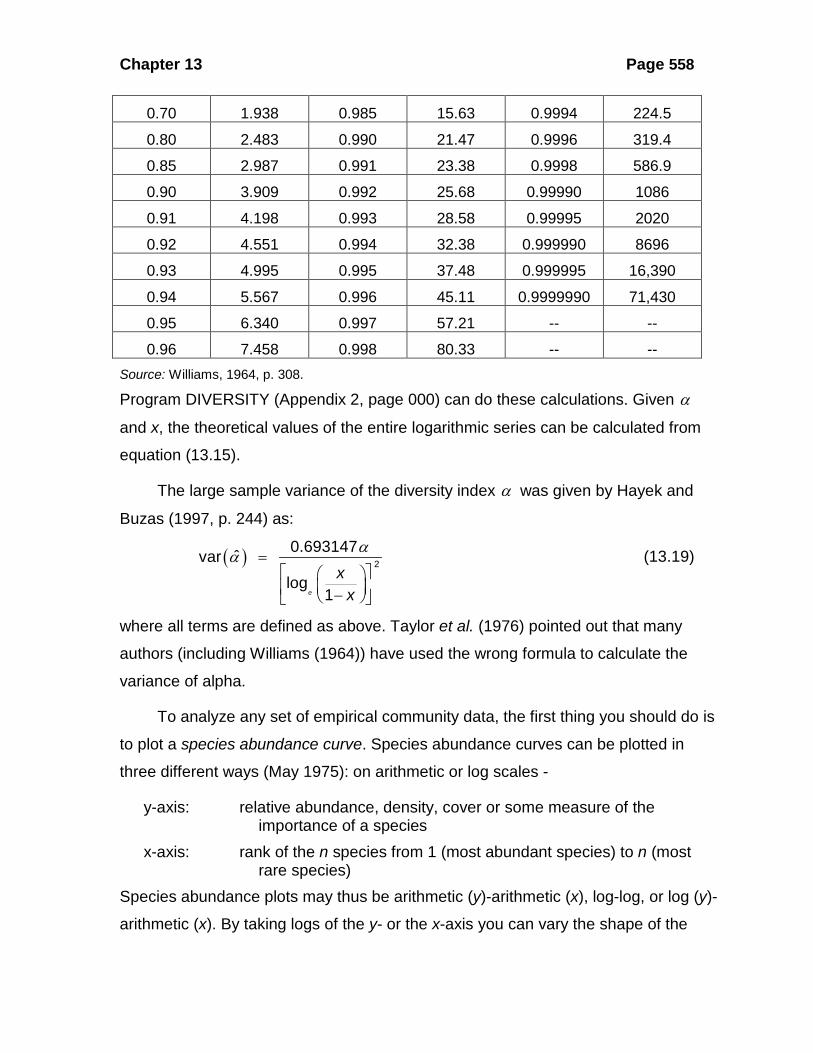
Chapter 13 Page 558
0.70 1.938 0.985 15.63 0.9994 224.5
0.80 2.483 0.990 21.47 0.9996 319.4
0.85 2.987 0.991 23.38 0.9998 586.9
0.90 3.909 0.992 25.68 0.99990 1086
0.91 4.198 0.993 28.58 0.99995 2020
0.92 4.551 0.994 32.38 0.999990 8696
0.93 4.995 0.995 37.48 0.999995 16,390
0.94 5.567 0.996 45.11 0.9999990 71,430
0.95 6.340 0.997 57.21 -- --
0.96 7.458 0.998 80.33 -- -- Source: Williams, 1964, p. 308. Program DIVERSITY (Appendix 2, page 000) can do these calculations. Given α
and x, the theoretical values of the entire logarithmic series can be calculated from
equation (13.15).
The large sample variance of the diversity index α was given by Hayek and
Buzas (1997, p. 244) as:
( ) 20.693147ˆvar log
1e
xx
αα =
−
(13.19)
where all terms are defined as above. Taylor et al. (1976) pointed out that many
authors (including Williams (1964)) have used the wrong formula to calculate the
variance of alpha.
To analyze any set of empirical community data, the first thing you should do is
to plot a species abundance curve. Species abundance curves can be plotted in
three different ways (May 1975): on arithmetic or log scales -
y-axis: relative abundance, density, cover or some measure of the importance of a species
x-axis: rank of the n species from 1 (most abundant species) to n (most rare species)
Species abundance plots may thus be arithmetic (y)-arithmetic (x), log-log, or log (y)-
arithmetic (x). By taking logs of the y- or the x-axis you can vary the shape of the

Chapter 13 Page 559
resulting curves. Figure 13.7 illustrates a standard plot of species abundances, after
Whittaker (1965). I call these Whittaker plots and recommend that the standard
species abundance plot utilize log relative abundance (y) - arithmetic species ranks
(x). The expected form of this curve for the logarithmic series is nearly a straight line
and is shown in Figure 13.7.
The theoretical Whittaker plot for a logarithmic series (e.g. Fig. 13.7(a)) can be
calculated as indicated in May (1975) by solving the following equation for n:
1 log 1eR E nNαα
= + (13.20)
where: Species rank ( axis, Figure 13.7)(i.e. 1, 2, 3, 4, , Index of diversity calculated in equation (12.18) Number of individuals expected for specified value
of ( axis of Figure 13.7) T
R x s
nR y
N
α===
=
1
otal number of individuals in sample Standard exponential integral (Abramowitz and Stegun, 1964, Chapter 5)E =
By solving this equation for n using integer values of R you can reconstruct the
expected Whittaker plot and compare it to the original data. Program DIVERSITY
(Appendix 2, page 000) has an option to calculate these theoretical values for a
Whittaker plot.
There is considerable disagreement in the ecological literature about the
usefulness of the logarithmic series as a good measure of heterogeneity. Taylor et
al. (1976) analyzed light trap catches of Macrolepidoptera from 13 sites in Britain,
each site with 6-10 years of replicates. They showed that the logarithmic series
parameter α was the best measure of species diversity for these collections. Hughes
(1986), by contrast, examined 222 samples from many taxonomic groups and
argued that the logarithmic series was a good fit for only 4% of these samples,
primarily because the abundant species in the samples were more abundant than
predicted by a logarithmic series. May (1975) attempted to provide some theoretical
justification for the logarithmic series as a description of species abundance patterns
but in most cases the logarithmic series is treated only as an empirical description of
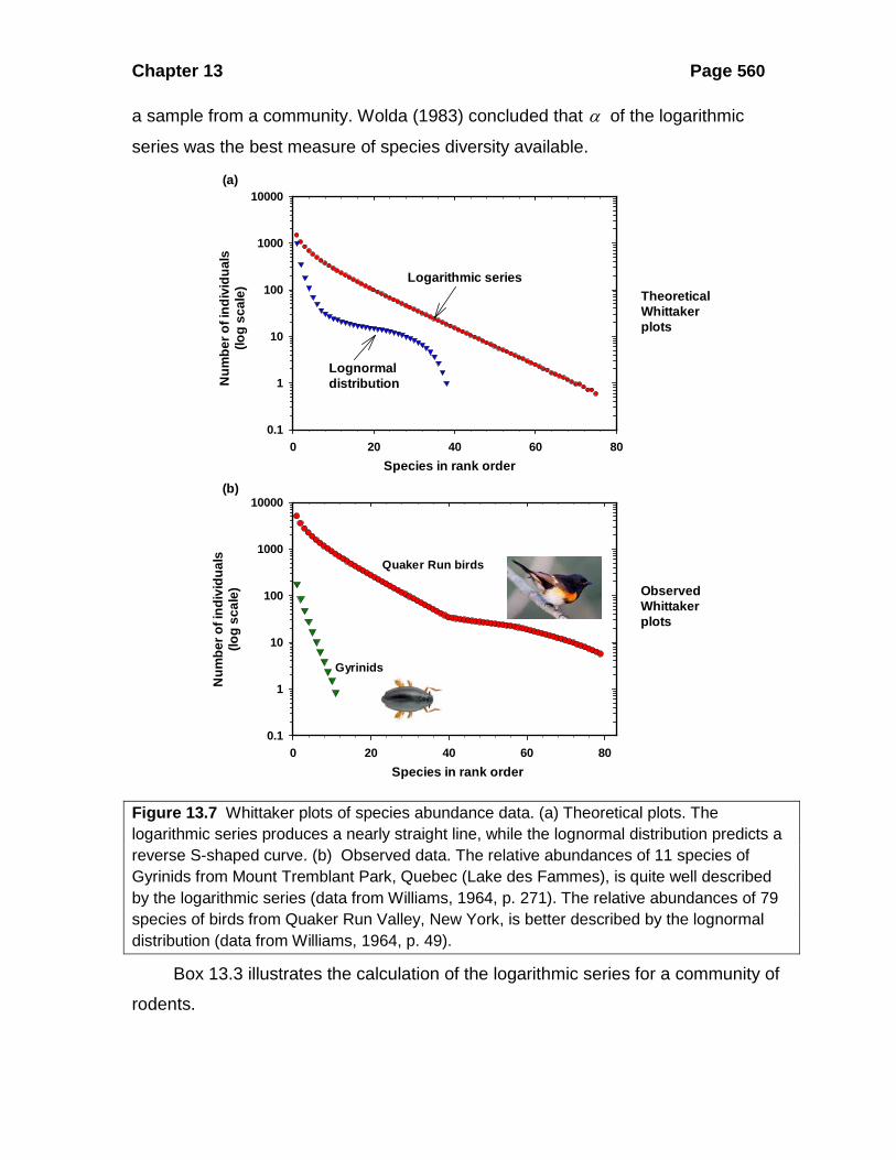
Chapter 13 Page 560
a sample from a community. Wolda (1983) concluded that α of the logarithmic
series was the best measure of species diversity available.
Figure 13.7 Whittaker plots of species abundance data. (a) Theoretical plots. The logarithmic series produces a nearly straight line, while the lognormal distribution predicts a reverse S-shaped curve. (b) Observed data. The relative abundances of 11 species of Gyrinids from Mount Tremblant Park, Quebec (Lake des Fammes), is quite well described by the logarithmic series (data from Williams, 1964, p. 271). The relative abundances of 79 species of birds from Quaker Run Valley, New York, is better described by the lognormal distribution (data from Williams, 1964, p. 49).
Box 13.3 illustrates the calculation of the logarithmic series for a community of
rodents.
Species in rank order0 20 40 60 80
Num
ber o
f ind
ivid
uals
(log
scal
e)
0.1
1
10
100
1000
10000
Logarithmic series
Lognormaldistribution
Theoretical Whittakerplots
Species in rank order0 20 40 60 80
Num
ber o
f ind
ivid
uals
(log
scal
e)
0.1
1
10
100
1000
10000
Observed Whittakerplots
Gyrinids
Quaker Run birds
(a)
(b)

Chapter 13 Page 561
Box 13.3 FITTING A LOGARITHMIC SERIES TO SPECIES ABUNDANCE DATA
Krebs and Wingate (1976) sampled the small-mammal community in the Kluane region of the southern Yukon and obtained these results:
No. of individuals
Deer mouse 498 Northern red-backed vole 495 Meadow vole 111 Tundra vole 61 Long-tailed vole 45 Singing vole 40 Heather vole 23 Northern bog lemming 5 Meadow jumping mouse 5 Brown lemming 4
N = 1287 S = 10
N/S = 128.7 From Table 13.3, an approximate estimate of x is 0.999. From equation (13.17) using this provisional estimate of x :
( )
( )
1 log 1
10 1 0.999 log 1 0.9991287 0.999
0.007770 0.006915
e
e
S x xN x
− = − − − = − −
≠
Since the term on the right side is too small, we reduce the estimate of x. Try 0.99898
( )1 0.998980.007770 log 1 0.998980.99898
0.007770 0.007033e
− = − − ≠
The right side of the equation is still too small, so we reduce x to 0.99888:
( )1 0.998880.007770 log 1 0.998880.99888
0.007770 0.0076183e
− = − − ≠
The right side of the equation is still slightly too small, so we repeat this calculation with

Chapter 13 Page 562
x = 0.998854 to obtain, using equation (13.17): 0.007770 0.007769
We accept 0.998854 as an estimate of the parameter x of the logarithmic series. From equation (13.18):
( )1287 1 0.998854ˆ
0.998854 1.4766
α−
=
=
The variance of this estimate of α is, from equation (13.19),
( ) 2 20.693147 0.693147 1.4766ˆvar 0.0307
0.998854log log1 1 0.998854e e
xx
αα ×= = =
− −
The individual terms of the logarithmic series are given by equation (13.15): 2 3
, , ,2 3x xx α αα
i
No. of species represented by i individuals
1 1.475 2 0.737 3 0.491 4 0.367 5 0.294 6 0.244 7 0.209
The sum of the terms of this series (which is infinite) is the number of species in the sample (S = 10). These data are used for illustration only. One would not normally fit a logarithmic series to a sample with such a small number of species. Program DIVERSITY (Appendix 2, page 000) can do these calculations.
The goodness of fit of the logarithmic series to a set of community data can be
tested by the usual chi-squared goodness of fit test (Taylor et al. 1976). But this chi-
squared test is of low power and thus many samples are accepted as fitting the
logarithmic series when it is in fact not a good fit (Routledge 1980). Thus in most
cases the decision as to whether or not to use the logarithmic series to describe the

Chapter 13 Page 563
diversity of a data set must be made on ecological grounds (Taylor et al. 1976,
Hughes 1986), rather than statistical goodness-of-fit criteria.
Koch (1987) used the logarithmic series to answer a critical methodological
question in paleoecology: If two samples are taken from exactly the same
community, how many species will be found in both data sets and how many
species will appear to be unique to one data set? Sample size effects may be critical
in paleoecological studies since absent species are typically classed as extinct.
Koch (1987) used the logarithmic series and simple probability theory to predict the
expected number of unique species in large samples from paleocommunities. These
predictions can serve as a null model to compare with observed differences between
samples. Figure 13.8 illustrates that the percentage of "unique species" can be very
large when samples differ in size, even when the samples are taken from the same
community. Rare species are inherently difficult to study in ecological communities,
and sample size effects should always be evaluated before differences are assumed
between two collections.
Figure 13.8 Use of the logarithmic series to predict the percentage of unique species in the larger of two data sets from exactly the same hypothetical community. Three values of α , the diversity parameter of the logarithmic series, are plotted to indicate low, moderate, and high diversity communities. The larger sample is 10,000 individuals. The point illustrates an independent sample of n = 2000 which is predicted to have about 45 unique species in spite
Sample size of smaller data set
1000 1500 2000 3000 4000 6000 8000 10000
Pred
icte
d no
. of u
niqu
e sp
ecie
s
0
10
20
30
40
50
60
50
400200

Chapter 13 Page 564
of being a sample from the identical community. These curves illustrate how difficult it is to sample the rare species in a diverse biological community. (Source: modified from Koch, 1987.)
13.4.2 Lognormal Distribution The logarithmic series implies that the greatest number of species has minimal
abundance, that the number of species represented by a single specimen is always
maximal. This is not the case in all communities. Figure 13.9 shows the relative
abundance of breeding birds in Quaker Run Valley, New York. The greatest number
of bird species are represented by ten breeding pairs, and the relative abundance
pattern does not fit the hollow-curve pattern of Figure 13.6. Preston (1948)
suggested expressing the X axis (number of individuals represented in sample) on a
geometric (logarithmic) scale rather than an arithmetic scale. One of several
geometric scales can be used, since they differ only by a constant multiplier; a few
scales are indicated in Table 13.4.
Figure 13.9 Relative abundance of nesting bird species in Quaker Run Valley, New York on a geometric scale with x3 size groupings (1-2, 3-8, 9-26, 27-80, 81-242, etc.). These data do not fit a hollow curve like that described by the logarithmic series. (Source: Williams, 1964.)
TABLE 13.4 GROUPINGS OF ARITHMETIC SCALE UNITS OF ABUNDANCE INTO GEOMETRIC SCALE UNITS FOR THREE TYPES OF GEOMETRIC SCALESa
No. of individuals - geometric classes
I II III IV V VI VII VIII
Num
ber o
f spe
cies
0
5
10
15

Chapter 13 Page 565
Geometric Arithmetic numbers grouped according to:
scale no. x2 Scaleb x3 Scalec x10 Scaled
1 1 1-2 1-9 2 2-3 3-8 10-99 3 4-7 9-26 100-999 4 8-15 27-80 1,000-9,999 5 16-31 81-242 10,000-99,999 6 32-63 243-728 100,000-999,999 7 64-127 729-2,186 -- 8 128-255 2,187-6,560 -- 9 256-511 6,561-19,682 --
a This type of grouping is used in Figure 12.6 b Octave scale of Preston (1948), equivalent to log2 scale. c Equivalent to log3 scale. d Equivalent to log10 scale.
When this conversion of scale is done, relative abundance data take the form
of a bell-shaped, normal distribution, and because the X axis is expressed on a
geometric or logarithmic scale, this distribution is called lognormal. The lognormal
distribution has been analyzed comprehensively by May (1975). The lognormal
distribution is completely specified by two parameters, although, as May (1975)
shows, there are several ways of expressing the equation:
01.772454ˆ TS S
a= (13.21)
where:
0
ˆ Total number of species in the community Parameter measuring the spread of the lognormal distribution Number of species in the largest class
TSa
S
===
The lognormal distribution fits a variety of data from surprisingly diverse communities
(Preston, 1948, 1962).
The shape of the lognormal curve is supposed to be characteristic for any
particular community. Additional sampling of a community should move the

Chapter 13 Page 566
lognormal curve to the right along the abscissa but not change its shape. Few
communities have been sampled enough to test this idea, and Figure 13.10 shows
some data from moths caught in light traps, which suggests that additional sampling
moves the curve out toward the right. Since we cannot collect one-half or one-
quarter of an animal, there will always be some rare species that are not
represented in the catch. These rare species appear only when very large samples
are taken.
Preston (1962) showed that data from lognormal distributions from biological
communities commonly took on a particular configuration that he called the
canonical distribution. Preston showed that for many cases a = 0.2 so that the entire
lognormal distribution could be specified by one parameter:
0ˆ 5.11422TS S= (13.22)
where:
0
ˆ = Total number of species in the community = Parameter measuring number of species in the modal (largest)
class of the lognormal as defined above
TSS

Chapter 13 Page 567
Figure 13.10 Lognormal distributions of the relative abundances of Lepidopteran insects captured in light traps at Rothamsted Experimental Station, England, in periods ranging from (a) 1/8 years to (b) 1 year to (c) 4 years. Note that the lognormal distribution sides to the right as the sample size is increased. (Source: Williams, 1964.)
Note that when the species abundance distribution is lognormal, it is possible
to estimate the total number of species in the community, including rare species not
yet collected. This is done by extrapolating the bell-shaped curve below the class of
minimal abundance and measuring the area. Figure 13.11 illustrates how this can be
I II III IV V VI VII VIII IX
No.
of s
peci
es
0
10
20
30
40
88 species492 individuals
(a)
I II III IV V VI VII VIII IX
No.
of s
peci
es
0
10
20
30
40
50
175 species3754 individuals
(b)
Geometric classes x3
I II III IV V VI VII VIII IX
No.
of s
peci
es
0
10
20
30
40
50
244 species16,065 individuals
(c)
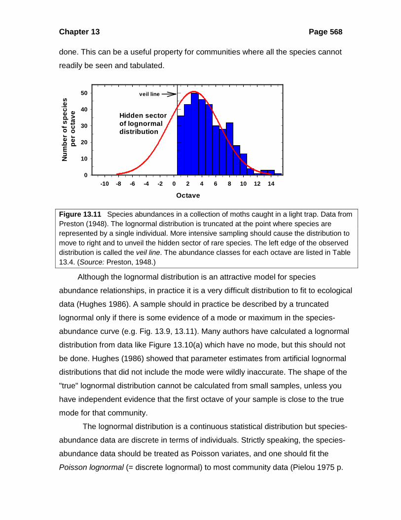
Chapter 13 Page 568
done. This can be a useful property for communities where all the species cannot
readily be seen and tabulated.
Figure 13.11 Species abundances in a collection of moths caught in a light trap. Data from Preston (1948). The lognormal distribution is truncated at the point where species are represented by a single individual. More intensive sampling should cause the distribution to move to right and to unveil the hidden sector of rare species. The left edge of the observed distribution is called the veil line. The abundance classes for each octave are listed in Table 13.4. (Source: Preston, 1948.)
Although the lognormal distribution is an attractive model for species
abundance relationships, in practice it is a very difficult distribution to fit to ecological
data (Hughes 1986). A sample should in practice be described by a truncated
lognormal only if there is some evidence of a mode or maximum in the species-
abundance curve (e.g. Fig. 13.9, 13.11). Many authors have calculated a lognormal
distribution from data like Figure 13.10(a) which have no mode, but this should not
be done. Hughes (1986) showed that parameter estimates from artificial lognormal
distributions that did not include the mode were wildly inaccurate. The shape of the
"true" lognormal distribution cannot be calculated from small samples, unless you
have independent evidence that the first octave of your sample is close to the true
mode for that community.
The lognormal distribution is a continuous statistical distribution but species-
abundance data are discrete in terms of individuals. Strictly speaking, the species-
abundance data should be treated as Poisson variates, and one should fit the
Poisson lognormal (= discrete lognormal) to most community data (Pielou 1975 p.
Octave-10 -8 -6 -4 -2 0 2 4 6 8 10 12 14
Num
ber o
f spe
cies
pe
r oct
ave
0
10
20
30
40
50
Hidden sectorof lognormaldistribution
veil line

Chapter 13 Page 569
49, Bulmer 1974). The Poisson lognormal is difficult to compute and Bulmer (1974)
has discussed methods of evaluating it. For practical purposes the ordinary
lognormal is usually fitted to species abundance data, using the maximum likelihood
methods devised by Cohen (1959, 1961)and described by Pielou (1975, pp. 50-53).
Gauch and Chase (1974) discussed a nonlinear regression method for fitting the
lognormal distribution to species abundance data, but Hansen and Zeger (1978)
showed that this regression method was not appropriate for species abundance
data, and recommended the method of Cohen.
To fit a lognormal distribution to species abundance data by the methods of
Cohen (1959, 1961) proceed as follows:
1. Transform all the observed data (number of individuals, or biomass, or other measure of species importance) logarithmically:
log i ix n= (13.23)
where:
0
Observed number of individuals of species in sample Species counter ( = 1, 2, 3, , ) * Transformed value for lognormal distribution
i
i
n ii i Sx
===
Any base of logarithms can be used, as long as you are consistent. I will use log-
base 10.
2. Calculate the observed mean and variance of xi by the usual statistical formulas (Appendix 1, page 000). Sample size is S0, the observed number of species.
3. Calculate the parameter y :
( )
2
20
syx x
=−
(13.24)
where:
2
0 10
Parameter of lognormal distribution Observed variance (calculated in step 2) Observed mean (calculated in step 2) log (0.5) 0.30103 if using log
ysx
x
==== = −
4. From Table 13.5 obtain the estimate of θ corresponding to this estimate of y.

Chapter 13 Page 570
5. Obtain corrected estimates of the mean and variance of the lognormal distribution from the equations:
( )0ˆ x x xµ θ= − − (13.25)
( )22 20ˆ s x xσ θ= + − (13.26)
where:
2
02
ˆ Estimate of true mean of the lognormal, Observed mean and variance from step 2
Correction factor from Table 13.5 (step 4) Truncation point of observed data log (0.5)
ˆ Estimate o
x s
x
µ
θ
σ
==== == f true variance of the lognormal
6. Calculate the standardized normal deviate corresponding to the truncation point:
00 xz µ
σ−
= (13.27)
7. From tables of the standard normal distribution (e.g. Rohlf and Sokal 1995, pg 78 or Zar 1996 Table B.2), find the area (p0) under the tail of the normal curve to the left of z0. Then:
0
0
ˆ 1T
SSp
=−
(13.28)
where:
0
0
ˆ Estimated number of species in the community(including those to the left of the veil line, e.g., Figure 13.11)
Observed number of species in sample Area of standard normal curve to left
TS
Sp
=
== 0of z
TABLE 13.5 VALUES OF THE ESTIMATION FUNCTION θ CORRESPONDING TOVALUES OF y OBTAINED IN EQUATION (13.24)a
y .000 .001 .002 .003 .004 .005 .006 .007 .008 .009 y
0.05 .00000 .00000 .00000 .00001 .00001 .00001 .00001 .00001 .00002 .00002 0.05
0.06 .00002 .00003 .00003 .00003 .00004 .00004 .00005 .00006 .00007 .00007 0.06
0.07 .00008 .00009 .00010 .00011 .00013 .00014 .00016 .00017 .00019 .00020 0.07
0.08 .00022 .00024 .00026 .00028 .00031 .00033 .00036 .00039 .00042 .00045 0.08
0.09 .00048 .00051 .00055 .00059 .00063 .00067 .00071 .00075 .00080 .00085 0.09
0.10 .00090 .00095 .00101 .00106 .00112 .00118 .00125 .00131 .00138 .00145 0.10

Chapter 13 Page 571
0.11 .00153 .00160 .00168 .00176 .00184 .00193 .00202 .00211 .00220 .00230 0.11
0.12 .00240 .00250 .00261 .00272 .00283 .00294 .00305 .00317 .00330 .00342 0.12
0.13 .00355 .00369 .00382 .00396 .00410 .00425 .00440 .00455 .00470 .00486 0.13
0.14 .00503 .00519 .00536 .00553 .00571 .00589 .00608 .00627 .00646 .00665 0.14
0.15 .00685 .00705 .00726 .00747 .00769 .00791 .00813 .00835 .00858 .00882 0.15
0.16 .00906 .00930 .00955 .00980 .01006 0.1032 .01058 .01085 .01112 .01140 0.16
0.17 .00168 .01197 .01226 .01256 .01286 .01316 .01347 .01378 .01410 .01443 0.17
0.18 .01476 .01509 .01543 .01577 .01611 .01646 .01682 .01718 .01755 .01792 0.18
0.19 .01830 .01868 .01907 .01946 .01986 .02026 .02067 .02108 .02150 .02193 0.19
0.20 .02236 .02279 .02323 .02368 .02413 .02458 .02504 .02551 .02599 .02647 0.20
0.21 .02695 .02744 .02794 .02844 .02895 .02946 .02998 .03050 .03103 .03157 0.21
0.22 .03211 .03266 .03322 .03378 .03435 .03492 .03550 .03609 .03668 .03728 0.22
0.23 .03788 .03849 .03911 .03973 .04036 .04100 .04165 .04230 .04296 .04362 0.23
0.24 .04429 .04497 .04565 .04634 .04704 .04774 .04845 .04917 .04989 .05062 0.24
0.25 .05136 .05211 .05286 .05362 .05439 .05516 .05594 .05673 .05753 .05834 0.25
0.26 .05915 .05997 .06080 .06163 .06247 .06332 .06418 .06504 .06591 .06679 0.26
0.27 .06768 .06858 .06948 .07039 .07131 .07224 .07317 .07412 ..7507 .07603 0.27
0.28 0.7700 .07797 .07896 .07995 .08095 .08196 .08298 .08401 .08504 .08609 0.28
0.29 .08714 .08820 .08927 .09035 .09144 .09254 .09364 .09476 .09588 .09701 0.29
0.30 .09815 .09930 .10046 .10163 .10281 .10400 .10520 .10641 .10762 .10885 0.30
0.31 .1101 .1113 .1126 .1138 .1151 .1164 .1177 .1190 .1203 .1216 0.31
0.32 .1230 .1243 .1257 .1270 .1284 .1298 .1312 .1326 .1340 .1355 0.32
0.33 .1369 .1383 .1398 .1413 .1428 .1443 .1458 .1473 .1488 .1503 0.33
0.34 .1519 .1534 .1550 .1566 .1582 .1598 .1614 .1630 .1647 .1663 0.34
0.35 .1680 .1697 .1714 .1731 .1748 .1765 .1782 .1800 .1817 .1835 0.35
0.36 .1853 .1871 .1889 .1907 .1926 .1944 .1963 .1982 .2001 .2020 0.36
0.37 .2039 .2058 .2077 .2097 .2117 .2136 .2156 .2176 .2197 .2217 0.37
0.38 .2238 .2258 .2279 .2300 .2321 .2342 .2364 .2385 .2407 .2429 0.38
0.39 ..2451 .2473 .2495 .2517 .2540 .2562 .2585 .2608 .2631 .2655 0.39
0.40 .2678 .2702 .2726 .2750 .2774 .2798 .2822 .2827 .2871 .2896 0.40
0.41 .2921 .2947 .2972 .2998 .3023 .3049 .3075 .3102 .3128 .3155 0.41
0.42 .3181 .3208 .3235 .3263 .3290 .3318 .3346 .3374 .3402 .3430 0.42
0.43 .3459 .3487 .3516 .3545 .3575 .3604 .3634 .3664 .3694 .3724 0.43
0.44 .3755 .3785 .3816 .3847 .3878 .3910 .3941 03973 .4005 .4038 0.44
0.45 .4070 .4103 .4136 .4169 .4202 .4236 .4269 .4303 .4338 .4372 0.45

Chapter 13 Page 572
0.46 .4407 .4442 .4477 .4512 .4547 .4583 .4619 .4655 .4692 .4728 0.46
0.47 .4765 .4802 .4840 .4877 .4915 .4953 .4992 .5030 .5069 .5108 0.47
0.48 .5148 .5187 .5227 .5267 .5307 .5348 .5389 .5430 .5471 .5513 0.48
0.49 .5555 .5597 .5639 .5682 .5725 .5768 .5812 .5856 .5900 .5944 0.49
0.50 .5989 .6034 .6079 .6124 .6170 .6216 .6263 .6309 .6356 .6404 0.50
0.51 .6451 .6499 .6547 .6596 .6645 .6694 .6743 .6793 .6843 .6893 0.51
0.52 .6944 .6995 .7046 .7098 .7150 .7202 .7255 .7308 .7361 .7415 0.52
0.53 .7469 .7524 .7578 .7633 .7689 .7745 .7801 .7857 .7914 .7972 0.53
0.54 .8029 .8087 .8146 .8204 .8263 .8323 .8383 .8443 .8504 .8565 0.54
0.55 .8627 .8689 .8751 .8813 .8876 .8940 .9004 .9068 .9133 .9198 0.55
0.56 .9264 .9330 .9396 .9463 .9530 .9598 .9666 .9735 .9804 .9874 0.56
0.57 .9944 1.001 1.009 1.016 1.023 1.030 1.037 1.045 1.052 1.060 0.57
0.58 1.067 1.075 1.082 1.090 1.097 1.105 1.113 1.121 1.1291 1.137 0.58
0.59 1.145 1.153 1.161 1.169 1.177 1.185 1.194 1.202 1.211 1.219 0.59
0.60 1.228 1.236 1.245 1.254 1.262 1.271 1.280 1.289 1.298 1.307 0.60
0.61 1.316 1.326 1.335 1.344 1.353 1.363 1.373 1.382 1.392 1.402 0.61
0.62 1.411 1.421 1.431 1.441 1.451 1.461 1.472 1.482 1.492 1.503 0.62
0.63 1.513 1.524 1.534 1.545 1.556 1.567 1.578 1.589 1.600 1.611 0.63
0.64 1.622 1.634 1.645 1.657 1.668 1.680 1.692 1.704 1.716 1.728 0.64
0.65 1.740 1.752 1.764 1.777 1.789 1.802 1.814 1.827 1.840 1.853 0.65
0.66 1.866 1.879 1.892 1.905 1.919 1.932 1.946 1.960 1.974 1.988 0.66
0.67 2.002 2.016 2.030 2.044 2.059 2.073 2.088 2.103 2.118 2.133 0.67
0.68 2.148 2.163 2.179 2.194 2.210 2.225 2.241 2.257 2.273 2.290 0.68
0.69 2.306 2.322 2.339 2.356 2.373 2.390 2.407 2.424 2.441 2.459 0.69
0.70 2.477 2.495 2.512 2.531 2.549 2.567 2.586 2.605 2.623 2.643 0.70
0.71 2.662 2.681 2.701 2.720 2.740 2.760 2.780 2.800 2.821 2.842 0.71
0.72 2.863 2.884 1.905 2.926 2.948 2.969 2.991 3.013 3.036 3.058 0.72
0.73 3.081 3.104 3.127 3.150 3.173 3.197 3.221 3.245 3.270 3.294 0.73
0.74 3.319 3.344 3.369 3.394 3.420 3.446 3.472 3.498 3.525 3.552 0.74
0.75 3.579 3.606 3.634 3.662 3.690 3.718 3.747 3.776 3.805 3.834 0.75
0.76 3.864 3.894 3.924 3.955 3.986 4.017 4.048 4.080 4.112 4.144 0.76
0.77 4.177 4.210 4.243 4.277 4.311 4.345 4.380 4.415 4.450 4.486 0.77
0.78 4.52 4.56 4.60 4.63 4.67 4.71 4.75 4.79 4.82 4.86 0.78
0.79 4.90 4.94 4.99 5.03 5.07 5.11 5.15 5.20 5.24 5.28 0.79
0.80 5.33 5.37 5.42 5.46 5.51 5.56 5.61 5.65 5.70 5.75 0.80

Chapter 13 Page 573
0.81 5.80 5.85 5.90 5.95 6.01 6.06 6.11 6.17 6.22 6.28 0.81
0.82 6.33 6.39 6.45 6.50 6.56 6.62 6.68 6.74 6.81 6.87 0.82
0.83 6.93 7.00 7.06 7.13 7.19 7.26 7.33 7.40 7.47 7.54 0.83
0.84 7.61 7.68 7.76 7.83 7.91 7.98 8.06 8.14 8.22 8.30 0.84
0.85 8.39 8.47 8.55 8.64 8.73 8.82 8.91 9.00 9.09 9.18 0.85
a These values are used to fit the lognormal distribution to species abundance data. Source: Cohen (1961). In the notation of equation (13.21), note that
2
1ˆ 2 ˆ
aσ
= (13.29)
where:
2ˆ Parameter measuring the spread of the lognormal distribution
ˆ True variance of the lognormal (equation 13.26)a
σ==
The variance of these estimates of the parameters of the lognormal distribution can
be estimated, following Cohen (1961), as:
( )2
11
0
ˆvar ˆ s
µ σµ = (13.30)
where:
( )112
0
var ˆ Estimated variance of mean of the lognormal Constant from Table 13.6
ˆ Estimate of true variance of lognormal (equation 13.26) Observed number of species in samples
µµσ
====
The variance of the standard deviation of the lognormal is given by:
( )2
22
0
ˆvar ˆ s
µ σσ = (13.31)
where:
( )22
2
0
var ˆ Variance of estimated standard deviation of the lognormal Constant from Table 13.6
ˆ True variance of lognormal Observed number of species in the samples
σµσ
====
These two variances may be used to set confidence limits for the mean and
standard deviation in the usual way. The goodness-of-fit of the calculated lognormal

Chapter 13 Page 574
distribution can be determined by a chi-square test (example in Pielou (1975) page
51) or by a nonparametric Kolmolgorov-Smirnov test.
Unfortunately there is no estimate available of the precision of ST (equation
13.23) and this is the parameter of the lognormal we are most interested in (Pielou
1975, Slocomb and Dickson 1978). Simulation work on artificial diatom communities
by Slocomb and Dickson (1978) showed that unreliable estimates of ST were a
serious problem unless sample sizes were very large (> 1000 individuals) and the
number of species in the sample were 80% or more of the total species in the
community. Such large-scale sampling is rare in the most species-rich communities
that we might wish to fit to the lognormal distribution.
Program DIVERSITY (Appendix 2, page 000) fits a truncated lognormal
distribution to species abundance data and calculates an expected distribution,
using the approach outlined in Pielou (1975).
Box 13.4 illustrates these calculations for a lognormal distribution.
Box 13.4 FITTING A TRUNCATED LOGNORMAL TO SPECIES ABUNDANCE DATA
Kempton and Taylor (1974) provided moth data for site 49, Fort Augustus, Scotland, in 1969; 4534 individuals were collected in 165 species:
Individuals per species
Midpoint of interval, x
Observed no. of species, fx
1 1 24 2-3 2.5 22 4-7 5.5 30 8-15 11.5 22 16-31 23.5 30 32-63 47.5 21 64-127 99.5 9 128-255 191.5 7
1. Calculate the mean and variance of the transformed data (log base 10) using the formulas for grouped data:
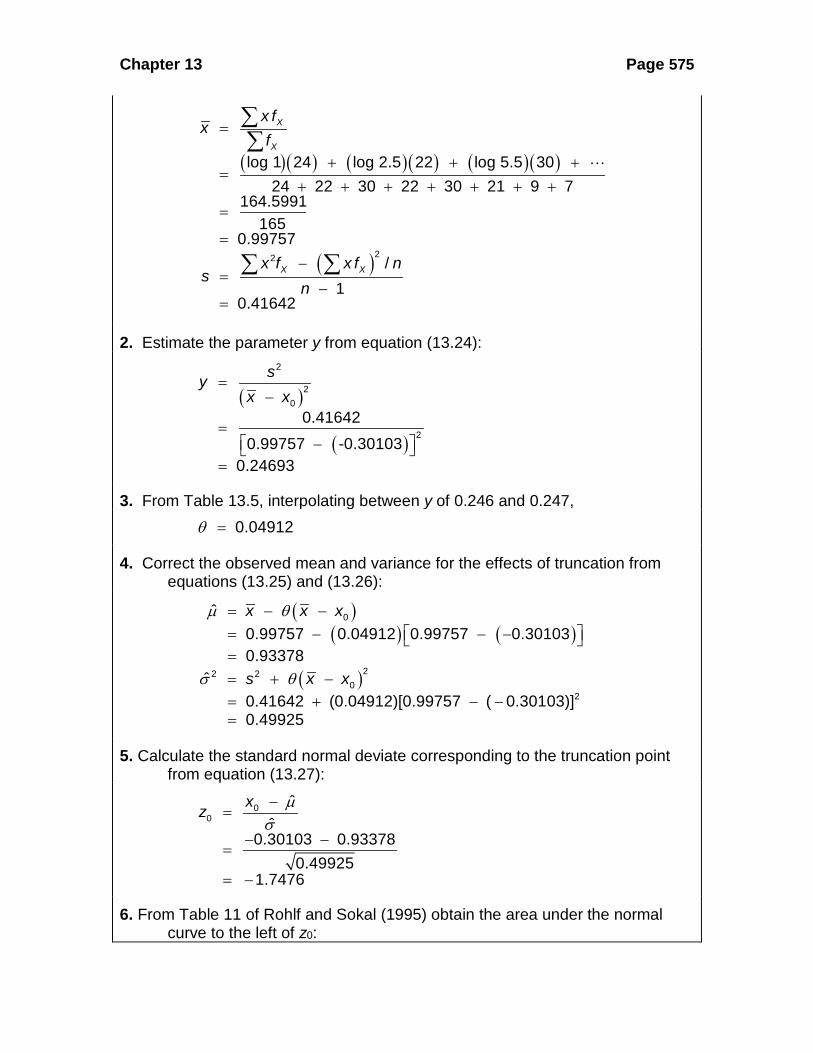
Chapter 13 Page 575
( )( ) ( )( ) ( )( )
( )22
log 1 24 log 2.5 22 log 5.5 30
24 22 30 22 30 21 9 7164.5991
165 0.99757
/
1 0.41642
X
X
X X
x fx
f
x f x f ns
n
=
+ + +=
+ + + + + + +
=
=−
=−
=
∑∑
∑ ∑
2. Estimate the parameter y from equation (13.24):
( )
( )
2
20
2
0.41642 0.99757 -0.30103
0.24693
syx x
=−
= −
=
3. From Table 13.5, interpolating between y of 0.246 and 0.247, 0.04912θ =
4. Correct the observed mean and variance for the effects of truncation from equations (13.25) and (13.26):
( )( ) ( )
( )
0
22 20
2
ˆ 0.99757 0.04912 0.99757 0.30103
0.93378ˆ 0.41642 (0.04912)[0.99757 ( 0.30103)] 0.49925
x x x
s x x
µ θ
σ θ
= − − = − − −
== + −= + − −=
5. Calculate the standard normal deviate corresponding to the truncation point from equation (13.27):
00
ˆ ˆ
0.30103 0.93378 0.49925
1.7476
xz µσ−
=
− −=
= −
6. From Table 11 of Rohlf and Sokal (1995) obtain the area under the normal curve to the left of z0:

Chapter 13 Page 576
0ˆ = 0.02005p
7. From equation (13.28) calculate the estimated number of species in the whole community:
0
0
ˆ1 165
1 0.02005 168.4 species
TSS
p=
−
=−
=
Kempton and Taylor (1974) cautioned that this fitting procedure may give inexact parameter estimates compared with Bulmer’s (1974) procedure.
13.4.3 Simpson's Index Partly because of the complexity of the logarithmic series and the lognormal
distribution and the lack of a theoretical justification for these statistical approaches,
ecologists have turned to a variety of non-parametric measures of heterogeneity that
make no assumptions about the shape of species abundance curves. The first non-
parametric measure of diversity was proposed by Simpson (1949). Simpson
suggested that diversity was inversely related to the probability that two individuals
picked at random belong to the same species. For an infinite population this is given
by:
2 iD p= ∑ (13.32)
where: Simpson's original index Proportion of species in the communityi
Dp i
==
To convert this probability to a measure of diversity, most workers have suggested
using the complement of Simpson's original measure:
Probability of picking twoSimpson's index of diversity = organisms at random that
are different speciesProbability of picking two
= 1 - organisms t
hat are thesame species

Chapter 13 Page 577
Thus:
( )21 1 iD p− = − ∑ (13.33)
where:
( )1 Simpson's index of diversity Proportion of individuals of species in the communityi
Dp i
− ==
Strictly speaking, this formula can be used to estimate Simpson's index only for an
infinite population. Pielou (1969) showed that, for a finite population the appropriate
estimator is:
( )( )1
1ˆ1 1 1
si i
i
n nD
N N=
−− = −
− ∑ (13.34)
where:
Number of individuals of species in the sample Total number of individuals in the sample Number of species in the sample
i
i
n iN ns
== ==
∑
Note that this formula (13.34) can be used only when there are counts of individuals
in the samples. When cover, biomass, or productivity are used as measures of
species importance, the previous equation (13.33) must be used. In practice with a
large sample there is almost no difference between these two equations.
There is some confusion in the literature over what should be called "Simpson's
Index". Washington (1984) argues strongly for maintaining Simpson's original
formulation, in which case equations (13.33) and (13.34) are the complement of
Simpson's diversity. To confuse matters further, Williams (1964) and MacArthur
(1972) used the reciprocal of Simpson's original formulation:
221 1 Hill's
i
ND p
= =∑
(13.35)
where:
21 Simpson's reciprocal index ( Hill's )
Proportion of species in the communityi
NDp i
= ==
Hill (1973) called this reciprocal N2. This index is now grouped under the rubric of
“Hill’s numbers” which are the preferred form of species diversity measures because
they are in units of species numbers. Simpson's index (1 - D) ranges from 0 (low

Chapter 13 Page 578
diversity) to almost 1 (1 - 1/s). Hill’s N2 or the reciprocal of Simpson's original
formulation (eq. 13.35) varies from 1 to s, the number of species in the sample. In
this form Hill’s N2 can be most easily interpreted as the number of equally common
species required to generate the observed heterogeneity of the sample.
Diversity is almost always measured by a sample from a community, and it is
virtually impossible for an ecologist to obtain a simple random sample (Pielou 1969,
Routledge 1980, 1980a). One way around this problem is to treat the community
sample as a collection, or a complete statistical `universe', and to make inferences
about this finite collection (Pielou 1966). Another approach is to use sampling units
such as quadrats for plants or nets for insects, and to estimate diversity using a
jackknife procedure. Zahl (1977) was the first to propose using this procedure to
provide confidence estimates for Simpson's diversity measure. Routledge (1980a)
showed that small samples (<30 quadrats) could give biased estimates for
Simpson's diversity (1 - D is underestimated), especially when less than 10 quadrats
were counted. Heltshe and Forrester (1985) suggested that the jackknife estimate of
confidence limits for Simpson's diversity (1 - D) was too large when applied to
clumped populations, causing excessively wide confidence limits when more than 40
quadrats were sampled in their artificial populations. This overestimation depended
on the exact shape of the species abundance curves.
Jackknife procedures for estimating Simpson's index of diversity and its
confidence limits from quadrat samples are outlined clearly in Routledge (1980a).
Lyons and Hutcheson (1986) proposed an alternative method for estimating
confidence limits for Simpson's diversity using Pearson curves, but there was little
improvement over the jackknife procedure. Program SPADE from Chao and Chen
(2010) calculates confidence intervals for Simpson’s index (1-D) and Hill’s N2.
13.4.4 Shannon-Wiener Function One of the most popular measures of species diversity was based on information
theory. The main objective of information theory is to try to measure the amount of
order (or disorder) contained in a system (Margalef 1958). Four types of information
might be collected regarding order in the community: (1) the number of species, (2)

Chapter 13 Page 579
the number of individuals in each species, (3) the places occupied by individuals of
each species, and (4) the places occupied by individuals as separate individuals. In
most community work only data of types (1) and (2) are obtained.
Information theory, Margalef suggested, provides one way to escape some of
the difficulties of the lognormal curve and the logarithmic series. We ask the
question: How difficult would it be to predict correctly the species of the next
individual collected? This is the same problem faced by communication engineers
interested in predicting correctly the next letter in a message. This uncertainty can
be measured by the Shannon-Wiener function*:
( )( )21
' - logs
i ii
H p p=
= ∑ (13.36)
where: ' Information content of sample (bits/individual)
Index of species diversity Number of species Proportion of total sample belonging to th speciesi
H
sp i
====
Chao and Shen (2003) adjusted the traditional Shannon-Wiener index to account for
the fact that some species are missed in the sample, and they suggested an
improved Shannon index:
( )( )
2
1
ˆ ˆlogˆˆ1 1
si i
ni i
p pH
p=
′ = −− −
∑ (13.37)
where all variables are defined above and n = total sample size
Equation (13.37) and (13.36) give very similar results for the Shannon-Wiener index
of diversity and we will use the adjusted Shannon measure (eq. 13.37) as the
recommended one for this index.
Information content is a measure of the amount of uncertainty, so that the
larger the value of H', the greater the uncertainty. A message such as bbbbbbb (or a
* This function was derived independently by Shannon and Wiener and is sometimes mislabeled the Shannon-Weaver function.
Chapter 13 Page 580
community with only one species in it) has no uncertainty in it, and H' = 0. Any base
of logarithms can be used for this index, since they are all convertible to one another
by a constant multiplier:
H' (base 2 logs) = 3.321928 H' (base 10 logs)
H' (base e logs) = 2.302585 H' (base 10 logs)
If base 2 logs are used, the units of H' are in bits per individual; if base e logs, nits;
and if base 10 logs, decits.
Strictly speaking, the Shannon-Wiener measure of information content should
be used only on random samples drawn from a large community in which the total
number of species is known (Pielou 1966). For most community samples this is not
the case, and Pielou (1966) thus recommends using the more appropriate Brillouin
index (see below, page 583).
The Shannon-Wiener measure H' increases with the number of species in the
community and in theory can reach very large values. In practice for biological
communities H' does not seem to exceed 5.0 (Washington 1984). The theoretical
maximum value is log (S), and the minimum value (when N>>S) is log (Fager
1972).
Many workers have used H' as a measure of species diversity, but the
information theoretic approach has been heavily criticized by Hurlbert (1971) and by
Washington (1984). The decision to use H' as a measure of species diversity should
be made more on empirical grounds than on theoretical grounds. For example,
Taylor et al. (1976) showed that α of the logarithmic series was a better diversity
statistic than H' because α varied less in replicate samples of moths taken at the
same site over several years. Many authors prefer Hill’s N2 (eq. 13.35) as the
simplest and most intuitive measure of heterogeneity.
Sampling distributions for the Shannon-Wiener index H' have been
determined by Good (1953) and Basharin (1959), but these standard errors of H' are
valid only if you have a simple random sample from the community. This is never the
case in field data where nets, traps, quadrats or transects are used for sampling
(Kempton 1979). Adams and McCune (1979) showed that estimates of H' from field
data are usually biased, so that observed H' is less than true H', and that the

Chapter 13 Page 581
jackknife technique could be used to reduce this bias and to estimate standard
errors for H' so that confidence limits might be calculated. Zahl (1977) and
Routledge (1980a) presented jackknife estimators for the Shannon-Wiener function
when data are collected by quadrat sampling. Chao and Shen (2010) provide
computer confidence limits for the Shannon Wiener index in Program SPADE.
The Shannon-Wiener index may be expressed in another form (MacArthur
1965) in units of numbers of species as a Hill’s number (N1):
1HN e ′= (13.38)
where:
1
1
2.71828 (base of natural logs)' Shannon-Wiener function (calculated with base logs) Number of equally common species which would produce
the same diversity as ' (Hill's )
eH eN
H N
≈==
If a different base of logs is used, replace e with the base of the logs used. Hill
(1973) recommends using N1 rather than H' because the units (number of species)
are more clearly understandable to ecologists. Peet (1974) recommends N1 as the
best heterogeneity measure that is sensitive to the abundances of the rare species
in the community.
Box 13.5 illustrates the calculation of Simpson's index, the Shannon-Wiener
index, and Brillouin’s index for a forest community.
Box 13.5 CALCULATION OF SIMPSON’S INDEX, THE SHANNON-WIENER INDEX, AND BRILLOUIN’S INDEX OF SPECIES DIVERSITY
Hough (1936) tallied the abundance of large trees in a virgin forest in Pennsylvania: Tree species No. of individuals
ni Proportional abundance
pi
Hemlock 1940 0.521 Beech 1207 0.324 Yellow birch 171 0.046 Sugar maple 134 0.036 Black birch 97 0.026 Red maple 93 0.025 Black cherry 34 0.009 White ash 22 0.006 Basswood 15 0.004 Yellow poplar 7 0.002 Magnolia 4 0.001

Chapter 13 Page 582
Total 3724 1.000
Simpson’s Index
From equation (13.32): 2
2 2 2 2
ˆ 0.521 0.324 0.046 0.0360.381
iD p== + + + +=
∑
The two indices of diversity follow from equations (13.33) and (13.35): ˆ1 1 0.381 0.619D− = − =
This measure is the probability that two individuals chosen at random will be different species.
1 1 2.623 speciesˆ 0.381D= =
This is the number of equally-common-species required to produce the observed value of D. Note that with this large sample the finite-population formula (eq. 13.34) gives results identical to equation (13.33).
Shannon-Wiener Index
From equation (13.33):
( )( )( )( ) ( )( ) ( )( )
21
2 2 2
ˆ ˆ' - log
0.521 log 0.521 0.324 log 0.324 0.046 log 0.0461.829 bits per individual
s
i ii
H p p=
=
= − + + +=
∑
Note that log2 (x) = 3.321981 log10 (x). The improved version of the Shannon-Wiener index (eq. 13.34) gives an identical value:
( )( )
2
1
ˆ ˆlog1.829 bits per individual
ˆ1 1
si i
ni i
p pH
p=
′ = − =− −
∑
From equation (13.38):

Chapter 13 Page 583
'
'
ˆ1
ˆ
1.829
ˆ (base logs)2 (base 2 logs)2 3.55 species
H
H
N e e=== =
Brillouin’s Index
From equation (13.39):
1 2 3
2
1 !ˆ log! ! !
1 3724!log 1.818 bits per individual 3724 1940!1207!171!134! 97!
NHN n n n
=
= =
Note that this is virtually identical to 'H .
Program DIVERSITY (Appendix 2, page 000) can do these calculations, as well as Program SPADE and Estimate S.
12.4.5 Brillouin’s Index Many community samples should be treated as collections rather than as a random
sample from a large biological community, according to Pielou (1966). In any case
in which the data can be assumed to be a finite collection, and sampling is done
without replacement, the appropriate information theoretic measure of diversity is
Brillouin's formula:
1 2 3
1 !ˆ log! ! !
NHN n n n
=
(13.39)
where:
1
2
ˆ Brillouin's index of species diversity Total number of individuals in entire collection Number of individuals belonging to species 1 Number of individuals belonging to species 2
HNnn
====
Any base of logarithms may be used, like the Shannon function. If base 2 logs are
used, the units of H are bits per individual. Margalef (1958) was the first to propose
using Brillouin's index as a measure of diversity.
There is much argument in the literature about whether the Brillouin index or
the Shannon-Wiener function is a better measure of species diversity (Peet 1974,

Chapter 13 Page 584
Washington 1984). In practice, this argument is irrelevant to field ecologists
because H and H' are nearly identical for most ecological samples (when N is large).
Legendre and Legendre (1983) also point out that Brillouin's index cannot be used
when biomass, cover, or productivity is used as a measure of species importance in
a community. Only the number of individuals can be used in equation (13.39).
If Brillouin’s index is applied to quadrats, the mean and standard error of
Brillouin’s index can be estimated by the jackknife procedure (Heltshe and Forrester
1985).
Brillouin’s index is like the Shannon function in being most sensitive to the
abundances of the rare species in the community. Peet (1974) recognized two
categories of diversity indices. Type I indices are most sensitive to changes in the
rare species in the community sample. The Shannon-Wiener index is an example of
a Type I index, like Brillouin’s index. Type II indices are most sensitive to changes in
the more abundant species. Simpson's index is an example of a Type II index. The
choice of what heterogeneity measure to use on your data should be made on this
basis - are you more interested in emphasizing the dominant or the rare species in
your community?
13.5 EVENNESS MEASURES Many different measures of evenness (or equitability) have been proposed and the
literature is most confusing about which measure is best. Smith and Wilson (1996)
have recently reviewed 14 indices of evenness with respect to the criterion that
evenness measures must be independent of species richness. The most common
approach has been to scale one of the heterogeneity measures relative to its
maximal value when each species in the sample is represented by the same number
of individuals. Two formulations are possible:
MAX
MIN
MAX MIN
Evenness
Evenness
DD
D DD D
=
−=
−
(13.40)
where:

Chapter 13 Page 585
MAX
MIN
Observed index of species diversity Maximum possible index of diversity, given
species and individuals Minimum possible index of diversity, given and
DD
S ND S N
==
=
These two measures (labeled V' and V by Hurlbert (1971)) are convergent for large
samples, and the first type of evenness measures (V' ) are most commonly used in
the literature. All these evenness measures should range from 0 to 1. Unfortunately
many of the indices of evenness based on this approach are not independent of
species richness, and other indices of evenness are needed. Smith and Wilson
(1996) prefer four indices:
13.5.1 Simpson’s Measure of Evenness For Simpson's measure of heterogeneity, maximum diversity is obtained when all
abundances are equal (p = 1/S) so in a very large population:
MAX1ˆ DS
= (13.41)
where:
MAXˆ Maximum possible value for Simpson's index (equation 13.32)
Number of species in the sampleD
S==
It follows from this that the maximum possible value of the reciprocal of Simpson’s
index (1/D) is always equal to the number of species observed in the sample. This
leads to a simple definition of Simpson’s index of evenness:
1
1ˆ
D
DES
= (13.42)
where:
1ˆ
Simpson's measure of evennessˆ Simpson's index (eq. 13.32)
number of species in the sample
DE
DS
=
==
This index ranges from 0 to 1 and is relatively unaffected by the rare species in the
sample.

Chapter 13 Page 586
13.5.2 Camargo’s Index of Evenness Camargo (1993) proposed a new index of evenness that is unaffected by species
richness and is simple to compute:
'
1 11..0
S Si j
i j i
p pE S
= = +
−= −
∑ ∑ (13.43)
where: ' Camargo's index of evenness
Proportion of species in total sampleProportion of species in total sampleNumber of species in total sample
i
j
Ep ip jS
====
This index like Simpson’s is relatively little affected by the rare species in the
sample.
13.5.3 Smith and Wilson’s Index of Evenness Smith and Wilson (1996) invented a new index of evenness which is based on the
variance in abundance of the species. The variance is measured over the log of the
abundances in order to use proportional differences rather than absolute differences
in abundance. The new index is defined as:
( ) ( )2S
e ei=1 1
var
log log /21 arctan
S
i jj
n n sE
sπ=
− = −
∑ ∑ (13.44)
where the arctangent is measured as an angle in radians and:
var Smith and Wilson's index of evennessNumber of individuals in species in sample ( 1, 2, 3, 4, ... )Number of individuals in species in sample ( 1, 2, 3, 4, ... )
Number of speci
i
j
En i i Sn j j Ss
== == == es in entire sample
This is the best available index of evenness, according to Smith and Wilson (1996),
because it is independent of species richness and it is sensitive to both rare and
common species in the community.
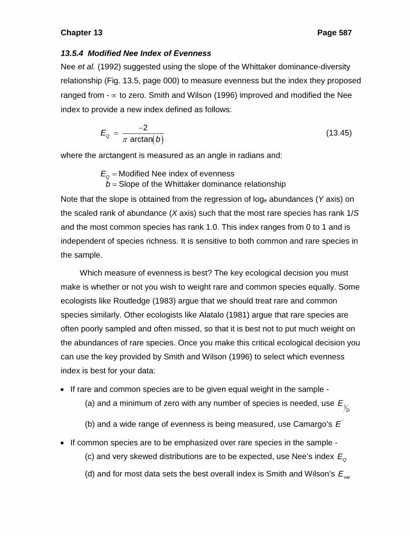
Chapter 13 Page 587
13.5.4 Modified Nee Index of Evenness Nee et al. (1992) suggested using the slope of the Whittaker dominance-diversity
relationship (Fig. 13.5, page 000) to measure evenness but the index they proposed
ranged from - ∝ to zero. Smith and Wilson (1996) improved and modified the Nee
index to provide a new index defined as follows:
( )2
arctanQEbπ
−= (13.45)
where the arctangent is measured as an angle in radians and:
Modified Nee index of evennessSlope of the Whittaker dominance relationship
QEb==
Note that the slope is obtained from the regression of loge abundances (Y axis) on
the scaled rank of abundance (X axis) such that the most rare species has rank 1/S
and the most common species has rank 1.0. This index ranges from 0 to 1 and is
independent of species richness. It is sensitive to both common and rare species in
the sample.
Which measure of evenness is best? The key ecological decision you must
make is whether or not you wish to weight rare and common species equally. Some
ecologists like Routledge (1983) argue that we should treat rare and common
species similarly. Other ecologists like Alatalo (1981) argue that rare species are
often poorly sampled and often missed, so that it is best not to put much weight on
the abundances of rare species. Once you make this critical ecological decision you
can use the key provided by Smith and Wilson (1996) to select which evenness
index is best for your data:
• If rare and common species are to be given equal weight in the sample -
(a) and a minimum of zero with any number of species is needed, use 1D
E
(b) and a wide range of evenness is being measured, use Camargo’s 'E
• If common species are to be emphasized over rare species in the sample - (c) and very skewed distributions are to be expected, use Nee’s index QE
(d) and for most data sets the best overall index is Smith and Wilson’s varE

Chapter 13 Page 588
There is a general problem with all measures of evenness - they all assume
you know the total number of species in the whole community (Pielou 1969). But this
number is almost always impossible to determine for species-rich communities.
Since observed species numbers must always be less than true species numbers in
the community, the evenness ratios are always overestimated (Sheldon 1969). Peet
(1974, 1975) and Routledge (1983) recommend that evenness measures should not
be used in ecological work unless the number of species in the whole community is
known. This is a very stringent restriction and is probably too purist. It may be
possible to know the total number of species in some temperate zone communities
and in well-studied tropical communities but this will be rare in most insect groups
and in other invertebrate taxa.
Program DIVERSITY (Appendix 2, page 000) calculates all these evenness
measures for species abundance data.
13.6 BETA-DIVERSITY MEASUREMENTS We have so far discussed ways to measure the species diversity of a single area or
community. These measures are collectively referred to as measures of α-diversity,
which is defined as the diversity of a defined habitat or community. Whittaker (1960)
was the first to recognize that there were other types of diversity measures that
might be useful. He described β-diversity as a measure of diversity that describes
how diversity changes as one moves across a diversity of communities. β-diversity
reflects species replacement as one moves across space or time (Magurran 2004).
Figure 13.12 illustrates Whittaker’s original concept of β-diversity from a set of tree
data along an elevation gradient in the mountains of southern Oregon.

Chapter 13 Page 589
Figure 13.12 Changes in species richness (α-diversity)at six elevations in the Siskiyou Mountains and the associated measure of species turnover or replacement (β-diversity) as elevation increases from 460 m to 2140 m. Species richness (α-diversity) was measured by the Chao 1 estimator (eq. 13.6), and species turnover (β-diversity) was estimated from (Source: Whittaker 1960 Table 12.)
There are two different conceptions of beta—diversity, the additive model and the
multiplicative model. Whittaker (1972) suggested the multiplicative model:
-diversity -diversity -diversityγ α β= × (13.46)
so that if you had a measure of alpha-diversity and gamma-diversity, you could get
beta-diversity from this equation by division. The additive model is:
-diversity -diversity + -diversityγ α β= (13.47)
so that you could get beta-diversity by subtraction. To complicate things further,
Anderson et al. (2011) pointed out that beta-diversity has been applied to two
conceptual models. The first is the change in species richness over an ecological
gradient, like the elevation on a mountain in Figure 13.12. The second is simply to
measure variation among samples within a study area. The key to selection of the
proper measure of beta-diversity is the ecological hypothesis or reason for the study.
Anderson et al. (2011) list 6 possible mission statements for studies of gradients,
Elevation (m)400 600 800 1000 1200 1400 1600 1800 2000 2200
Spec
ies
richn
ess
0
5
10
15
20
25
Spec
ies
turn
over
0.0
0.1
0.2
0.3
0.4
0.5
0.6
0.7
alpha-diversitybeta-diversity

Chapter 13 Page 590
and another 6 mission statements for studies of variation among samples. The
methods of analysis and conclusions differ depending on exactly what question you
are asking. Chao et al. (2012) suggested a resolution to these differences of
definition along the same lines by pointing out that measures of species diversity
that include only presence/absence data are difficult to compare because of
undetected rare species, while measures of diversity that include species
abundance measures (like the Morisita-Horn measure) are easier to estimate
because they are most sensitive to the abundant species in the samples.
There does not exist and I doubt that there will soon be a simple resolution to
discussions about how to measure beta-diversity. Magurran (2004) provides a useful
starting guide. Detailed discussions of some ways to proceed in this area are given
in Chao et al. (2012) and Colwell et al. (2012). At present rarefaction methods for
comparisons may be the simplest and most direct approach. The key point is that we
are interested in testing ecological hypotheses and the methods must be tailored to
the hypotheses, rather than vice versa.
13.7 RECOMMENDATIONS There has been more attention paid in community ecology to the measurement of
species diversity than to almost any other parameter. There is thus an enormous
literature on diversity, full of contradictory recommendations. In some respects the
problems of measuring diversity are similar to the problems of measuring similarity.
Following Magurran (2004), I suggest it would be best to take an empirical approach
as follows:
1. Measure species abundance by abundance, biomass, or cover if possible.
Presence/absence data can be utilized but are sensitive to undetected rate species.
2. Construct Whittaker plots of log abundance on species rank (Figure 13.5) with the
abundance data. The shape of the dominance-diversity curve will indicate which
models of species-abundance relations might be applied to the data.
3. Estimate species richness using the rarefaction method (Figure 13.2). This will
permit the comparison of species richness among several communities sampled
with different intensity.

Chapter 13 Page 591
3. Fit the logarithmic series or the lognormal curve to the data, if the Whittaker plot
indicates this is reasonable. The logarithmic series α may be a useful index of
diversity even for communities which deviate from the logarithmic distribution.
4. Use Hill’s numbers as easily interpreted measures of diversity. This includes the
reciprocal of Simpson's index (Hill’s N2, eq. 13.35) or the exponential form of the
Shannon-Wiener function (Hill’s N1, eq. 13.38) to describe heterogeneity. You
should decide beforehand whether you wish to weight the common species more
(Simpson's) or the rare species more (Shannon's) in your community analysis.
5. Use Smith and Wilson’s index of evenness (eq. 13.44) to estimate evenness for
the community sample, unless you have good data on both the rare species and the
common ones (in which case use Camargo’s 'E ).
Practical wisdom is still accumulating in community ecology about which
indices of diversity are most useful for specific applications (Anderson et al. 2011,
Chao et al. 2012, Colwell et al. 2012). It is clear that there will be no one universal
approach that can be recommended for all communities, and much more empirical
work is required.
13.8 SUMMARY Species diversity is a dual concept that includes the number of species in the
community, their abundance, and the evenness with which the individuals are
divided among the species. To describe and compare different communities,
ecologists recognize three components – alpha, beta, and gamma diversity. Alpha
diversity is local diversity while gamma diversity is the total regional diversity of a
large area. Beta diversity links alpha and gamma diversity, or local and regional
diversity. There are many ways of measuring species diversity, and much
controversy about which indices of diversity are "best".
Species richness, or the number of species in the community, is easy to
determine only in easily censused communities with few species. In all other cases,
the larger the sample size, the longer the species list. The rarefaction technique
allows one to adjust a series of samples to a common sample size (no. individuals)
so that species richness can be compared among samples. For quadrat sampling a

Chapter 13 Page 592
jackknife estimate of species richness can be made, based on the number of
species that occur in only one quadrat.
Heterogeneity measures confound species richness and evenness in a single
index of diversity. Two statistical distributions have been commonly fitted to species
abundance data - the logarithmic series and the lognormal distribution. Non-
parametric measures of heterogeneity are commonly used because they assume no
statistical distribution. Type I heterogeneity measures place most weight on the rare
species in the sample, and the Shannon-Wiener function is an example of these
measures. Type II heterogeneity measures place most weight on the common
species, and Simpson's index is an example of these.
Evenness can be estimated in many different ways, and the key concept is to
relate observed species abundances to maximum possible heterogeneity, when all
species have an equal abundance. Good measures of evenness are now available
once you have decided whether to emphasize or de-emphasize the rare species in
your community samples.
SELECTED REFERENCES Chao, A., et al. 2006. Abundance-based similarity indices and their estimation when
there are unseen species in samples. Biometrics 62 (2): 361-371. Chiarucci, A. 2012. Estimating species richness: still a long way off! Journal of
Vegetation Science 23(6): 1003-1005. Colwell, R. K., et al. 2012. Models and estimators linking individual-based and
sample-based rarefaction, extrapolation and comparison of assemblages. Journal of Plant Ecology 5(1): 3-21.
Ellison, A. M. 2010. Partitioning diversity. Ecology 91(7):1962-1963. Harte, J., A. B. Smith, and D. Storch. 2009. Biodiversity scales from plots to biomes
with a universal species–area curve. Ecology Letters 12(8): 789-797. Magurran, A. E. 2004. Measuring Biological Diversity. Blackwell Publishing, Oxford.
256pp. Magurran, A. E. and B. J. McGill, (eds.) 2011. Biological Diversity : Frontiers in
Measurement and Assessment. Oxford University Press, New York. 346pp. Mao, C.X. and J. Li. 2009. Comparing species assemblages via species
accumulation curves. Biometrics 65:1063–7.

Chapter 13 Page 593
Smith, B. and J.B. Wilson. 1996. A consumer’s guide to evenness indices. Oikos 76: 70-82.
Xu, H., S. et al. 2012. Assessing non-parametric and area-based methods for estimating regional species richness. Journal of Vegetation Science 23(6): 1006-1012.
QUESTIONS AND PROBLEMS 13.1 Calculate a rarefaction curve for a sample of a subalpine forest community
containing 278 individual trees in 7 species as follows: ES, 126; SF, 103; LP, 27; PC, 12; AL, 6; DF, 2; and AF, 2. Estimate a 95% confidence interval for species richness at a sample size of 100 individuals.
13.2 Use the jackknife estimator of species richness to estimate the total richness of herbs in an Indiana oak-hickory forest from the following set of 17 quadrats:
Quadrat 1
Species 1 2 3 4 5 6 7 8 9 10 11 12 13 14 15 16 17
A 13 5 1 7 12 2 2 4 6 7 1 4
B 4 1 1 6 2 4 1 7 8 9 12 2 7
C 2 7 1 3 8 1 2 1 7 1 2 2 1 1
D 1
E 6 5 1 7 12 6 7 2 3 1 4 1 1 6 5
F 1
G 1
H 3 1 7 6 1 2 3 4 2 1 1 7 1 4 2
I 6
J 1 4 12 1 3 8 6 4 2 1 1 3 2 1 7 4 2
13.3 Fit the logarithmic series to Patrick's (1968) diatom data for Box 7 given in Table 13.1, page 554. Graph the theoretical and the observed species abundance data in a Whittaker plot, and do a chi-square goodness-of-fit test on these data.
13.4 Fit the lognormal distribution to these same diatom data of Patrick's, and discuss whether the canonical lognormal is a good description of this data set.
13.5 Fit the lognormal distribution to the data on moths given in Kempton and Taylor (1974: Journal of Animal Ecology 43, Table 4, page 391). Compare the estimated parameters with those given in that paper, and discuss why they differ.
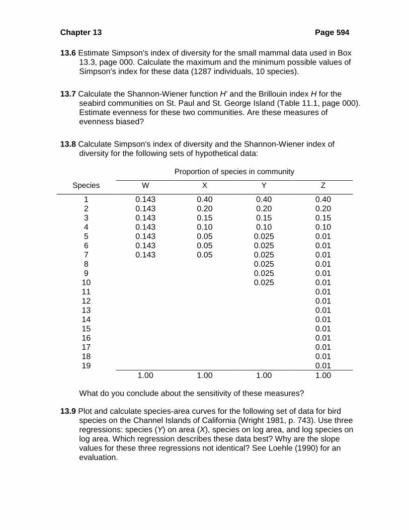
Chapter 13 Page 594
13.6 Estimate Simpson's index of diversity for the small mammal data used in Box 13.3, page 000. Calculate the maximum and the minimum possible values of Simpson's index for these data (1287 individuals, 10 species).
13.7 Calculate the Shannon-Wiener function H' and the Brillouin index H for the seabird communities on St. Paul and St. George Island (Table 11.1, page 000). Estimate evenness for these two communities. Are these measures of evenness biased?
13.8 Calculate Simpson's index of diversity and the Shannon-Wiener index of diversity for the following sets of hypothetical data:
Proportion of species in community
Species W X Y Z
1 0.143 0.40 0.40 0.40 2 0.143 0.20 0.20 0.20 3 0.143 0.15 0.15 0.15 4 0.143 0.10 0.10 0.10 5 0.143 0.05 0.025 0.01 6 0.143 0.05 0.025 0.01 7 0.143 0.05 0.025 0.01 8 0.025 0.01 9 0.025 0.01
10 0.025 0.01 11 0.01 12 0.01 13 0.01 14 0.01 15 0.01 16 0.01 17 0.01 18 0.01 19 0.01
1.00 1.00 1.00 1.00
What do you conclude about the sensitivity of these measures?
13.9 Plot and calculate species-area curves for the following set of data for bird species on the Channel Islands of California (Wright 1981, p. 743). Use three regressions: species (Y) on area (X), species on log area, and log species on log area. Which regression describes these data best? Why are the slope values for these three regressions not identical? See Loehle (1990) for an evaluation.

Chapter 13 Page 595
Island Area (km2) Bird species
Santa Barbara 2.6 10
Anacapa 2.8 14
San Miguel 36 15
San Nicholas 57 11
San Clemente 145 24
Santa Catalina 194 34
Santa Rosa 218 25
Santa Cruz 249 37
13.10 Calculate evenness indices for the four recommended evenness measures for the hypothetical two species communities suggested by Alatalo (1981) and used by Molinari (1989):
Community Species X abundance Species Y abundance
A 999 1
B 900 100
C 800 200
D 700 300
E 600 400
F 500 500
The expectation is that the index of evenness should respond in a reasonable way to this gradual change in evenness. Plot the shapes and discuss which indices fulfill this expectation. Smith and Wilson (1996, p. 79) discuss this criterion.
13.11 Wilson et al. (2012) extrapolated the species-area curve for observed data on vascular plants (quadrats up to 1 km2) to the area of the entire terrestrial biosphere (130 million km2) in order to determine the total number of vascular plants on earth. Review their approach and the success of their extrapolation.