chapter 14 a linear nonequilibrium thermodynamics approach ... · 14 a linear nonequilibrium...

Chapter 14A Linear Nonequilibrium ThermodynamicsApproach to Optimization of ThermoelectricDevices

Henni Ouerdane, Christophe Goupil, Yann Apertet, Aurélie Michotand Adel Abbout

Abstract Improvement of thermoelectric systems in terms of performance andrange of applications relies on progress in materials science and optimization ofdevice operation. In this chapter, we focus on optimization by taking into accountthe interaction of the system with its environment. For this purpose, we considerthe illustrative case of a thermoelectric generator coupled to two temperature bathsvia heat exchangers characterized by a thermal resistance, and we analyze its work-ing conditions. Our main message is that both electrical and thermal impedancematching conditions must be met for optimal device performance. Our analysis isfundamentally based on linear nonequilibrium thermodynamics using the force-fluxformalism. An outlook on mesoscopic systems is also given.

H. Ouerdane · C. Goupil · (B) · A. AbboutLaboratoire CRISMAT, UMR 6508 CNRS, ENSICAEN et Université de CaenBasse Normandie, 6 Boulevard Maréchal Juin, F-14050 Caen, Francee-mail: [email protected]

H. Ouerdane · C. GoupilSorbonne Paris Cité, Institut des Energies de Demain (IED),Université Paris Diderot, 75205 Paris, Francee-mail: [email protected]

A. Abboute-mail: [email protected]

Y. ApertetInstitut d’Electronique Fondamentale, Université Paris-Sud, CNRS, UMR 8622,F-91405 Orsay, Francee-mail: [email protected]

A. MichotCNRT Matériaux UMS CNRS 3318, 6 Boulevard Maréchal Juin, F-14050 Caen Cedex, Francee-mail: [email protected]

K. Koumoto and T. Mori (eds.), Thermoelectric Nanomaterials, Springer Series 323in Materials Science 182, DOI: 10.1007/978-3-642-37537-8_14,© Springer-Verlag Berlin Heidelberg 2013

324 H. Ouerdane et al.

14.1 Introduction

At the standard macroscopic scale various technologies exist for waste energy har-vesting and conversion: heat exchangers for energy storage and routing, heat pumps,organic Rankine cycle, and thermoelectricity. Depending on the specific work-ing conditions, one technology may be viewed as more efficient than another; forinstance, thermoelectricity is more appropriate in cases where the temperature dif-ference between the heat source and sink is not too large. Efforts are invested in theimprovement of thermoelectric devices in terms of properties and range of applica-tions because their conversion efficiency is not size-dependent and the typical devicedoes not contain moving parts. These qualities, of paramount importance in viewof applications at the mesoscale in the microelectronics industry, recently provideda new impetus for research in the field of thermoelectricity . Tremendous progressin the understanding and mastering of thermoelectric systems has been made sincethe pioneering works of Seebeck [1] and Peltier [2], but much remains to be donein order to improve the energy conversion efficiency at maximum output power.Indeed, even at the macroscale the best energy conversion efficiency of thermoelec-tric devices typically are of the order of 10% of the efficiency of the ideal Carnotthermodynamic cycle.

A “good” thermoelectric material has a large thermopower and a high electricalconductivity to thermal conductivity ratio. The properties of a given material mayusually be qualified as good in a very limited range of temperatures though. Recentadvances in the physics and engineering of semiconductors and strongly correlatedmaterials have permitted great progress by way of optimization of the materials’characteristics, thus offering interesting prospects for device performance and rangeof operation. But, with practical purposes in mind, one must consider that a realdevice is not a perfect theoretical system, and that its thermal contacts, through heatexchangers, with the temperature reservoirs are usually far from ideal too. A poordevice design and neglect of the quality of the thermal contacts can only yield poordevice performance however good is the thermoelectric material. This clearly meansthat there are a number of truly important technological challenges which must bemet; high quality brazing is one of them. From a theoretical/modeling viewpoint,it is also necessary to develop models that capture the essential characteristics ofthermoelectric devices operating in realistic working conditions. Indeed, to make thebest possible use of the best materials available, one needs to understand how theinternal laws of a device may be appropriately associated to the laws that govern itsinteraction with its environment. We propose here a reflection along these lines.

The link between the intrinsic properties of a thermoelectric device and its perfor-mance usually is given by the so-called figure of merit. While much work is devotedto find means to increase the figure of merit, our present work rather focuses on howto achieve optimal working conditions. Thermoelectric devices can be described asheat engines connected to two temperature reservoirs. In these systems, transport ofheat and transport of electric charges are strongly coupled. Not too far from equilib-rium these transport phenomena obey linear phenomenological laws such as those

14 A Linear Nonequilibrium Thermodynamics Approach 325

Table 14.1 Examples of linear phenomenological laws

Variables Transport coefficient Expression and name

Electrical current density and electric field Electrical conductivity J = σE ≡ −σ∇ϕ

Ohm’s lawParticle flux and density Diffusion coefficient J N = −D∇n

Fick’s lawEnergy flux and temperature Thermal conductivity J E = −κ∇T

Fourier’s law

given in Table14.1; so a general macroscopic description of thermoelectric systemsis in essence phenomenological. Linear nonequilibrium thermodynamics providesa most convenient framework to characterize the device properties and the workingconditions to achieve various operation modes. As we shall see in this chapter theapproximations we make, which are well controlled, are used to obtain analyticalexpressions that facilitate the analysis, discussion and understanding of the physicalconcepts we study.

Our approach, presentedhere for amodel of a thermoelectric generator non-ideallycoupled to the temperature reservoirs through finite-conductance heat exchangers,is quite an appropriate starting point for an extension down to mesoscopic scale.Assuming a simple resistive load and introducing an effective thermal conductancefor the device, we show first that, in addition to electrical impedance matching,conditions that permit thermal impedance matching must be also satisfied in order toachieve optimal device performance. The problem of efficiency at maximum poweris central in our work, but it becomes quite tricky as soon as it is addressed at afundamental level. It is fortunate that the model system we study allows derivationof simple formulas at the cost of approximations that are perfectly reasonable in theframework of linear response.

The thermodynamic formulation that we use is that of Callen1 [3]: in its modernform, due to Callen in 1960, the equilibrium thermodynamics can be summarizedby the main postulate of the existence of an entropy maximum. The postulates,which will be detailed in the next section, assume an understanding of: (1) thedistinctions between macroscopic and microscopic variables, and between extensiveand intensive macroscopic variables; (2) the concept of a system surrounded byboundaries that restrict, i.e. hold constant, some or all of the extensive variablesof the system; (3) the definitions of internal energy U and work done on a systemW , and the concept of heat Q, defined through the first law of thermodynamics:δQ = dU − δW .

We start this Chapter with a recap of linear nonequilibrium thermodynamics: abrief overview of some of the basics concepts and tools developed by Onsager [4, 5]

1 For convenience, Callen formulates the postulates of thermodynamics only for simple systems,defined as systems that are large enough, macroscopically homogeneous, isotropic and uncharged;the surface effects can be neglected, and no external electric, magnetic, or gravitational fields actson these systems.


and Callen [6] is necessary to set the scenery. A short presentation of thermoelectriceffects in absence of magnetic fields will follow. We will see that the force-fluxformalism provides a net description of thermoelectric processes [7]. Then, we willturn to our analysis of device optimization. The Chapter ends with a discussion onefficiency at maximum power, and an outlook on thermoelectricity at the mesoscopicscale.

14.2 Basic Notions of Linear Nonequilibrium Thermodynamics

For the sake of clarity in the next sections of the chapter, it is useful at this stageto start from the basic definitions and notions. Before getting into nonequilibriumphysics, it is useful to remind here some notions concerning equilibrium.

A thermodynamic system is usually defined as a collection of a great numberof objects characterized by fundamental quantities called extensive and intensivevariables that describe its macroscopic properties. A thermodynamic state is definedby the specification of some macroscopic physical properties of the system (all theproperties are not necessary for a study). Therefore one physical system may corre-spond to many thermodynamic systems. We will precise these points below, whenthe postulates of equilibrium statistical mechanics are stated.

To each set of extensive variables associated to a thermodynamic system, thereis a counterpart, i.e. a set of intensive variables. The thermodynamic potentials areconstructed from these variables. For example, for a gas of noninteractingmolecules,onemayconsider the following extensive variables: entropy S, volumeV , andparticlenumber N , and their coupled intensive variables: temperature T , pressure P , andchemical potential μ. The internal energy, which is a thermodynamic potential, isgiven by: U = T S − PV + μN . The thermodynamic equilibrium is obtained whenthermal, mechanical, and chemical equilibria are reached. This may be reformulatedas follows: an equilibrium state is reached when all the thermodynamic potentialsare minimum. This implies that if the thermodynamic system is in equilibrium, allthe parts of this system are in equilibrium.

14.2.1 Postulates and Origin of Irreversibilities

Thermodynamics is useful to describe equilibrium states, but physical processes arerather characterized by irreversibility and nonequilibrium states. A thermodynamicdescription of equilibrium states may only yield very incomplete information onthe actual processes at work, and thus needs to be extended to account for the ratesof the physical processes. Irreversible thermodynamics provides links between themeasurable quantities, and nonequilibrium statistical physics provides the tools tocompute these.


The framework of nonequilibrium statistical mechanics is essentially rooted inthree postulates, two of which concern equilibrium:

1. A thermodynamic system, isolated and in equilibrium, is characterized by a verylarge number of accessiblemicrostates; spontaneous transitions occur continuallybetween these microstates.

2. Each of the accessible microstates has equal a priori probability.

For a given system, the ensemble of microstates with same energy forms a statisticalensemble called a microcanonical ensemble. The a priori probability relates to theprinciple of indifference: during the course of its evolution, an isolated system in anequilibrium statewill experience all the accessiblemicrostates at the same recurrencerate. Therefore, one may assume that the average of a physical quantity over longtimes is equal to the average of the same quantity over the microcanonical ensemble.In other words, for a stationary system, there is an equivalence between the perform-ing of many identical measurements on a single system and a single measurementon many replicas of the system. This is the ergodic hypothesis.

The third postulate, in its simplest form reads:

3. Time symmetry of physical laws: in absence of applied magnetic or Coriolisforce fields, their mathematical formulation remains unchanged if the time t iseverywhere replaced by −t .

The state of a macroscopic system is defined by its macroscopic parameters, buta macrostate gives no information about the state of an individual component; soif the macroscopic properties of two stationary systems take the same values, thesetwo systems are thermodynamically indistinguishable. The probability that a certainmacrostate is realized is determined by the number of microstates that correspond tothis macrostate; this number is called the multiplicity of the given macrostate. Sincethermodynamic systems are large, macrostates multiplicities are immensely large.Some macrostates are more probable than others so, in a nutshell, irreversibility ofprocesses in macroscopic systems appears as the evolution from the less probable tothe more probable configuration in phase space.

Now, why are some macrostates more probable than others? As a matter of fact,irreversibility emerges as a result of different but tightly connected factors [8]. Thefirst of these is the very large number of degrees of freedom in a thermodynamicsystem. A direct consequence of this large number is that the relation between theprobability of the thermodynamic system to be in a macrostate and the occupiedphase space volume can only be based on probabilistic arguments. Moreover, thetrajectories in phase space are extremely sensitive to the conditions in which thesystem was initially prepared by application of some constraints; this implies that,after the lifting of some or all of the said constraints, the dynamics that drives therelaxation of the system towards an equilibrium state is by essence chaotic, andhence, in the course of the system evolution, the probability to pass again throughthe initial macrostate can only decrease and come to be extremely small. Thougharguments against irreversibility such as Zermelo’s paradox based on Poincaré’srecurrence, and Loschmidt’s paradox based on microreversibility were put forward,


it is obvious that on the one hand, a Poincaré’s recurrence time is overwhelminglylarge for a thermodynamic system and, on the other hand, there is no such thing asa real, perfectly isolated system: perturbations, as small as they may be but strictlynonzero, are unavoidable.

14.2.2 Principle of Maximum Entropy and Time Scales

At the macroscopic scale, the equilibrium states of a systemmay be characterized bya number of extensive variables Xi . If the system is composed of several subsystems,relaxation of some constraints yields changes in the values taken by the variables Xi ,which correspond to the exchanges between the subsystems. For each equilibriumstate, one may define a function S that is positive, continuous and differentiable withrespect to the variables Xi :

S : Xi �→ S(Xi ) (14.1)

The function S, called entropy, is extensive: S is the sum of the entropies ofthe subsystems. The values finally taken by the variables Xi after relaxation ofconstraints, are those which characterize equilibrium, and which correspond to themaximum of the function S.

The extensive variables Xi , macroscopic by nature, also differ from the micro-scopic variables because of the typical time scales over which they evolve: the relax-ation time of the microscopic variables being extremely fast, the variables Xi maybe qualified as slow in comparison. In fact, one may distinguish four well separatedtime scales:

1. The duration of one single collision, τ02. The collision time,which is the typical timewhichpasses between twoconsecutive

collision events, τcol3. The relaxation time towards local equilibrium τrelax4. The time necessary for the evolution towards the macroscopic equilibrium, τeq.

These characteristic times satisfy the following inequalities:

τ0 � τcol � τrelax � τeq (14.2)

Therefore, since the variables Xi are slow, one may define an instantaneousentropy, S(Xi ), at each step of the relaxation of the variables Xi . The differential ofthe function S is:

dS =∑

i

∂S

∂XidXi =

∑

i

FidXi , (14.3)

where each quantity Fi is the intensive variable conjugate of the extensive variable Xi .


14.2.3 Forces and Fluxes

The notions which follow are best introduced in the case of a discrete system.2

Now assume an isolated system composed of two weakly coupled sub-systems towhich an extensive variable taking the values Xi and X ′

i , is associated. One has:

Xi + X ′i = X (0)

i = constant and S(Xi ) + S(X ′i ) = S(X (0)

i ). Then, the equilibriumcondition maximizing the total entropy is given by:

∂S(0)

∂Xi

∣∣∣X (0)

i

= ∂(S + S′)∂Xi

dXi

∣∣∣X (0)

i

= ∂S

∂Xi− ∂S′

∂X ′i

= Fi − F ′i = 0 (14.4)

The equation above tells us that if the differenceFi = Fi − F ′i is zero, the system

is in equilibrium; otherwise an irreversible process takes place and drives the systemto equilibrium. The quantityFi thus acts as a generalized force (or affinity) allowingthe evolution of the system towards equilibrium. In addition, we introduce the rateof variation of the extensive variable Xi , which characterizes the response of thesystem to the applied force:

Ji = dXi

dt(14.5)

And we see that a given flux cancels if its conjugate affinity cancels. Conversely,a non-zero affinity yields a non-zero conjugated flux. In other words, the relationshipbetween affinities and fluxes characterizes the changes due to irreversible processes.

14.2.4 Entropy Production and Local Equilibrium

For a given out-of-equilibrium system, it is useful to study the rate of variation ofthe total entropy in order to determine the appropriate forces and fluxes. Retainingthe same notation as above, we have:

dS(0)

dt=

∑

i

∂S(0)

∂Xi

dXi

dt(14.6)

This rate of variation also is called entropy production. It can be rewritten as:

dS(0)

dt=

∑

i

Fi Ji (14.7)

2 One may imagine for instance two separate homogeneous systems initially prepared at two differ-ent temperatures and then put in thermal contact through a thin diathermal wall. The thermalizationprocess will trigger a flow of energy from on system to the other.


This rate exhibits a bilinear structure: it is the sum of the products of each flux byits conjugate affinity. Note that this property can be generalized to continuous media.

Large systems may be treated as continuous media, which are assumed to be inequilibrium locally. More precisely, a systemmay be divided in cells of intermediatesize, i.e. small enough so that the variables vary only little, but large enough to beconsidered as thermodynamical sub-systems in contact with their environment. Itis then possible to define local thermodynamical quantities that are uniform withineach separate cell, but different from one cell to another. With the assumption oflocal equilibrium, the local entropy σ(r), as a function of local thermodynamicalquantities, has the same form as the entropy S and the local intensive variables aredefined as functional derivatives of S. Note that the local equilibrium cells are opento energy and matter transport

14.2.5 Entropy Balance and Miminum Entropy Theorem

Entropy is an extensive quantity that is not conserved. The global balance for entropyreads:

dS

dt= −

∫

�

JS · n d� +∫

VσSd

3r ≡ dSexchdt

+ dSintdt

, (14.8)

where dSexch/dt is the contribution todS/dt due to entropy exchangebetween the sys-tem and its environment (thermostat) and dSint/dt is the entropy production relatedto the internal changes of the system. The quantities JS and σS are the entropy fluxand the entropy source respectively. The entropy production characterizes the rateof variation of the entropy of the global system: {system;environment}. Irreversiblephenomena that contribute to an entropy production are called dissipative phenom-ena.

In some circumstances, non-equilibrium states are steady states in the sense thatthey are characterized by state variables Xi which are time-independent. In this case,we can write:

dS

dt= dSexch

dt+ dSint

dt= 0 (14.9)

and, sincedSintdt

=∫

VσSd

3r ≥ 0 (14.10)

then dSexch/dt ≤ 0. This implies that in order to maintain a system in a non-equilibrium steady state, entropy must continually be transferred from this systemto its environment. As shown by Prigogine [9] in 1945, the non-equilibrium steadystates correspond to aminimum of entropy production since in a time-dependent sys-tem, the rate of entropy production can only decrease monotonically as the systemapproaches equilibrium.


14.2.6 Linear Response and Reciprocal Relations

In a continuous medium in local equilibrium, the fluxes depend on their conjugateaffinity (direct effect), but also on the other affinities (indirect effect). At a given pointin space and time (r, t), the flux Ji can be mathematically defined as dependent onthe force Fi , but also on the other forces F j =i :

Ji (r, t) ≡ Ji (F1,F2, . . .) (14.11)

Close to equilibrium, Ji (r, t) can be written as a Taylor expansion:

Jk(r, t) =∑

j

∂ Jk

∂F jF j + 1

2!∑

i, j

∂2 Jk

∂FiF jFiF j +· · · =

∑

k

L jkFk + 1

2

∑

i, j

Li jkFiF j +· · ·

(14.12)The quantities L jk are the first-order kinetic coefficients; they are given by the equi-librium values of the intensive variables Fi . The matrix [L] of the kinetic coefficientscharacterizes the linear response of the system.

In the linear regime, the source of entropy reads:

σS =∑

i,k

LikFiFk (14.13)

Since σS ≥ 0, the kinetic coefficients satisfy

Lii ≥ 0 and Lii Lkk ≥ 1

4(Lik + Lki ) (14.14)

If some processes induce rapid variations of the affinities in space and time, therecannot be any local equilibrium. The kinetic coefficients of linear theory acquirea non-local and a retarded character: the fluxes at a given point and a given time,depend on the affinities at other points in space, and at previous times.

In 1931, Onsager [4, 5] put forward the idea that there exist symmetry and anti-symmetry relations between kinetic coefficients: the so-called reciprocal relationsmust exist in all thermodynamic systems for which transport and relaxation phe-nomena are well described by linear laws. The main results can be summarized asfollows [10]:

• Onsager’s relation: Lik = Lki

• Onsager-Casimir relation: Lik = εi εk Lki

• generalized relations: Lik(H,�) = εi εk Lki (−H,−�)

where H and � respectively denote a magnetic field and an angular velocity asso-ciated to a Coriolis field; the parameters εi denote the parity with respect to timereversal: if the quantity studied is invariant under time reversal transformation, ithas parity +1; otherwise this quantity changes sign, and it has parity −1. Onsager’s


reciprocal relations are rooted in the reversibility of the microscopic equations ofmotion.

The response of a system upon which constraints are applied, is the generationof fluxes which correspond to transport phenomena. When the constraints are lifted,relaxation processes drive the system to an equilibrium state. Energy dissipation andentropy production are associated to transport and relaxation processes.

14.3 Forces and Fluxes in Thermoelectric Systems

14.3.1 Thermoelectric Effects

A naive definition would state that thermoelectricity results from the coupling ofOhm’s law and Fourier’s law. The thermoelectric effect in a system may rather beviewed as the result of themutual interference of two irreversible processes occurringsimultaneously in this system, namely heat transport and charge carrier transport. Inthermoelectricity, three effects are usually described:

1. The Seebeck effect, which is the rise of an electromotive force in a thermocouple,i.e. across a dipole composed of two conductors forming two junctionsmaintainedat different temperatures, under zero electric current.

2. The Peltier effect, which is a thermal effect (absorption or production of heat) atthe junction of two conductors maintained at the same temperature.

3. The Thomson effect, which is a thermal effect that goes together with the steadyelectrical current that flows through a resistive dipole because of the existence ofa temperature gradient applied to the dipole.

It is important to realize here that these three “effects” all boil down to the sameprocess: At themicroscopic level, an applied temperature gradient causes the chargesto diffuse,3 so the Seebeck, Peltier and Thomson effects are essentially the same phe-nomenon, i.e. thermoelectricity, which manifests itself differently as the conditionsfor its observation vary. Broadly speaking, when a temperature difference is imposedacross a thermoelectric device, it generates a voltage, and when a voltage is imposedacross a thermoelectric device, it generates a temperature difference. The thermo-electric devices can be used to generate electricity, measure temperature, cool orheat objects. For a thermocouple composed of two different materials A and B, thevoltage is given by:

VAB =∫ T2

T1(αB − αA)dT, (14.15)

where the parameters αA/B are the Seebeck coefficients or thermopowers.

3 One may see an analogy with a classical gas expansion.


14.3.2 The Onsager–Callen Model

The main assumption of Onsager’s work is based on the hypothesis that the systemevolution is driven by a minimal production of entropy where each fluctuation ofany intensive variable undergoes a restoring force to equilibrium [11]. This permitsthe use of a stationary description with a clear definition of all the thermodynamicalpotentials, though the system itself produces dissipation. From a thermodynamicpoint of view this is no more than a definition of a quasi-static process since thesystem is considered to back to local equilibrium at each time. This leads to thevery important result that the classical quasi-static relation between heat and entropyvariation dS = δQqs/T may be extended to finite time response thermodynamics inthe following flux form:

JS = JQ

T(14.16)

which allows a continuous thermodynamical description of the system: the ther-modynamical equilibrium, with all average fluxes equal to zero, just becomes onepossible thermodynamical state for the system.

The domain of validity of Onsager’s description is thus limited to processes whereentropy production is always minimal. By minimal we do not mean that the systemwill always take the overall minimal entropy production state, but only the minimalentropy production with respect to the external applied constraints, which are calledworking conditions. These may be fulfilled or not, leading to an overall minimalentropy production that can be very far from its optimal value. Finally one maynotice that Onsager’s description is no more than a generalization of the fluctuation-dissipation theorem,which assumes that the linear response of a system in a stationarystate, and the noisy response of this system are related through the same underlyingmechanisms [10–13].

14.3.3 Coupled Fluxes

The Onsager force-flux derivation is obtained from the consideration of the laws ofconservation of energy and matter. The expression of the relation between the energyflux JE , the heat flux JQ , and the particle flux JN :

JE = JQ + μe JN (14.17)

is established by application of the first principle of thermodynamics. Each of thesefluxes is the conjugate variable of its thermodynamic potential gradients. In the caseof an electron gas, the correct potentials for energy and particles are respectively 1/Tand μe/T , and the corresponding forces are: FN = ∇(−μe/T ) and FE = ∇(1/T ).Then the linear coupling between forces and fluxes may simply be described by alinear set of coupled equations involving the so-called kinetic coefficient matrix [L]:


[JN

JE

]=

[LNN LNE

LEN LEE

] [∇(−μeT )

∇( 1T )

](14.18)

where LNE = LEN .The symmetry of the off-diagonal terms is a fundamental aspect of Onsager’s

analysis, since it is equivalent to a minimal entropy production of the system in out-of-equilibrium conditions. It should be noticed that the minimal entropy productionis not a general property of out-of-equilibrium processes at all so that Onsager’sassumption should be present inside the kinetic matrix [L]. It is known from linearresponse theory that linear response and fluctuations inside a dissipative system areclosely linked. Then each of the fluctuating potentials experiences a restoring forcederived from the others in a symmetric form. From a purely thermodynamic pointof view this coincides with the Lechatelier-Braun principle. The equality LNE =LEN is nothing else but the manifestation of the intrinsic symmetry of the coupledfluctuations process. From a microscopic point of view this equality also implies thetime reversal symmetry of the processes.4 By extension, at the microscopic scaleprocesses should be “microreversible”, and “irreversible thermodynamics” becomes“reversible dynamics”.

14.3.4 Energy Flux and Heat Flux

To treat properly heat and electrical currents it is more convenient to consider JQ

instead of JE as the pertinent quantity to be analyzed. Using JE = JQ + μe JN weobtain: [

JN

JQ

]=

[L11 L12L21 L22

] [− 1T ∇(μe)

∇( 1T )

](14.19)

with L12 = L21. Since ∇(−μe/T ) = −μe∇(1/T ) − 1/T ∇(μe) the heat andelectronic currents read:

[JN

JQ

]=

[LNN LNE − μeLNN

LNE − μeLNN −2LNEμe + LEE + μ2eLNN

] [∇(−μeT )

∇( 1T )

](14.20)

with the following relationship between kinetic coefficients:

L11 = LNN (14.21)

L12 = LNE − μeLNN (14.22)

L22 = LEE − 2μeLEN + μ2eLNN (14.23)

Note that since the electric field derives from the electrochemical potential wealso obtain

4 This time reversal symmetry is broken under the application of Coriolis or magnetic forces.


E = −∇(μe)

e(14.24)

14.4 Thermoelectric Coefficients

The thermoelectric coefficients can be derived from the expressions of the elec-tronic and heat flux densities depending on the applied thermodynamic constraints:isothermal, adiabatic, electrically open or closed circuit conditions.

14.4.1 Decoupled Processes

Under isothermal conditions the electrical current flux may be written in the form,

JN = −L11

T∇(μe) (14.25)

This is an expression of the law of Ohm since with J = e JN we obtain the followingrelationship between the electrical current density and the electric field:

e JN = J = e−L11

T∇(μe) = σT

(−∇(μe)

e

)= σT E, (14.26)

which contains a definition for the isothermal electrical conductivity expressed asfollows:

σT = e2

TL11 (14.27)

Now, if we consider the heat flux density in the absence of any particle transportor, in other words, under zero electrical current, we get:

JN = 0 = −L11

(1

T∇(μe)

)+ L12∇(

1

T) (14.28)

so that the heat flux density under zero electrical current, JQ J=0 , reads:

JQ J=0 = 1

T 2

[L21L12 − L11L22

L11

]∇(T ) (14.29)

This is the law of Fourier, with the thermal conductivity under zero electrical currentgiven by


κJ = 1

T 2

[L11L22 − L21L12

L11

](14.30)

We can also define the thermal conductivity κE under zero electrochemical gra-dient, i.e. under closed circuit conditions:

JQE=0 = L22

T 2 ∇(T ) = κE∇(T ) (14.31)

It follows that the thermal conductivities κE and κJ are simply related through:

κE = T α2σT + κJ (14.32)

14.4.2 Coupled Processes

Let us now shed some light on the coupled processes. In the absence of any electrontransport, the basic expression is already known since it is given by Eq. (14.28). Wemay now define the Seebeck coefficient as the ratio between the two forces thatderive from the electrochemical and temperature potentials:

α ≡ − 1e ∇(μe)

∇(T )= 1

eT

L12

L11(14.33)

Under an isothermal configuration the coupling term between electronic currentdensity and heat flux is obtained from the two following expressions:

J = e JN = eL11

(− 1

T∇(μe)

)(14.34)

JQ = L21

(− 1

T∇(μe)

)(14.35)

which yield a definition of the Peltier coefficient �:

JQ = 1

e

L12

L11J = �J (14.36)

Now the equality� = T α (14.37)

is obvious. The close connexion between Peltier and Seebeck effects is illustratedby this compact expression. In echo to what was said at the begining of Sect. 14.3,this shows, from a fundamental point of view, that all thermoelectric effects are infact different expressions of the same quantity SJ , called the “ entropy per carrier ”


defined by Callen [3]:SJ = αe (14.38)

14.4.3 Kinetic Coefficients and General Expression for the Lawof Ohm

The analysis and calculations developed above allow to establish a complete corre-spondence between the kinetic coefficients and the transport parameters:

L11 = σT

e2T (14.39)

L12 = σT SJ T 2

e2(14.40)

L22 = T 3

e2σT S2

J + T 2κJ (14.41)

so that the expressions for the electronic and heat currents may take their final forms:

JN = σT

e2T

(−∇(μe)

T

)+ σT SJ T 2

e2

(∇(

1

T)

)(14.42)

JQ = σT SJ

e2T 2

(−∇(μe)

T

)+

[T 3

e2σT S2

J + T 2κJ

] (∇(

1

T)

)(14.43)

Since J = e JN , it follows that

J = σT E − σT SJ

e∇(T ) (14.44)

from which we obtain:E = ρT J + α∇(T ) (14.45)

where ρT is the isothermal conductivity. This is a general expression of the law ofOhm.

14.4.4 The Dimensionless Figure of Merit ZT

The off-diagonal terms of the kinetic matrix [L] represent the coupling between theheat and the electrical fluxes. The question is now to consider the way to optimizea given material in order to get an efficient heat pump driven by an input electricalcurrent or electrical generators driven by a heat flux. The procedure can be derived


for both applications, and we propose here to consider the case of a thermoelectricgenerator (TEG).

Let us first look at the optimization of the fluxes. Since a thermoelectric systemis an energy conversion device, the more heat that flows into the material, the moreelectrical power may be produced. In order to achieve this, we expect a large ther-mal conductivity for the material. Unfortunately, this will also lead to a very smalltemperature difference and consequently a small electrical output voltage and power.This configuration can be called the short-circuit configuration since the fluxes aremaximized and the differences of the potentials minimized.

Let us now consider the coupled processes from the potential point of view. Inorder to get the larger voltage, the material should experience a large temperaturedifference between its edges. Then the thermal conductivity of the material shouldbe as small as possible, leading to a very small heat flux and consequently, again,a small electrical output power. This configuration can be called the open-circuitconfiguration since the potential differences aremaximized and the fluxesminimized.

It is worth noticing that both short-circuit and open-circuit configurations leadto an unsatisfactory situation. Moreover they are in contradiction since the thermalconductivity is expected to be maximum in the short-circuit configuration and min-imum in the open-circuit one. The relationship between the thermal conductivitiesderived above, and written again here:

κE = T α2σT + κJ

offers a way to solve this contradiction. Since it was established under zero currentcondition, the conductivity κJ corresponds to the open-circuit configuration whilethe conductivity κE corresponds to the short-circuit configuration. From the pre-vious developments we expect the ratio κE/κJ to be maximal to get the maximaloutput electrical power from the TEG. The explicit expression of the ratio containsa definition of the figure of merit Z T :

κE

κJ= α2σT

κJT + 1 = Z T + 1 (14.46)

A maximal value of the ratio κE/κJ implies that reaching the highest possiblevalue of Z T is a necessary condition to qualify amaterial as optimal. The thermoelec-tric properties of the material are summarized in the figure of merit Z T , as proposedby Ioffe [14]. This quantity gives a quantitative information on the quality of thematerial, and hence for practical applications. Since only the material parametersenter into its expression, the figure of merit is clearly the central term for materialengineering research. In addition it should be noticed that the present description doesnot consider at all the anions of the crystal lattice of the thermoelectric material butonly the electronic gas.5 This is due to the Onsager description which follows the lin-ear response theory that does not include the lattice contribution to heat conduction.

5 An analogue situation would be considering a steam engine without any boiling walls.


However, this contribution may be accounted for in the general conductance matrixby considering a parallel path for the heat flux.

14.5 Device Optimization: Case of a Thermoelectric Generator

14.5.1 Device Characteristics

We consider a single-leg module with section s and length L placed between twoheat reservoirs that act as thermostats. The proposed thermogenerator configurationincludes the presence of heat exchangers, one between the hot thermostat at temper-ature Thot and the hot side module, the other between the cold side of the module andthe cold thermostat at temperature Tcold. It should be noticed that this configurationcannot be reduced to a simpler one limited to the module, since the hot side, ThM, andcold side, TcM, module temperatures may vary during the operation of the module.

We assume that the two thermal contacts on both sides of the module are com-pletely characterized by the constant thermal conductances Kcold and Khot. The totalcontact conductance, Kcontact, is K −1

contact = K −1cold + K −1

hot . An extension to varyingthermal conductances may be considered in the case of non-linear convection orradiative processes. For the sake of simplicity we restrict our analysis to constantheat exchangers thermal conductances. It should also be mentioned that in the caseof very efficient heat exchangers, it is tempting to fully neglect their presence andconsider a perfect coupling to the thermostats. This consideration is wrong by prin-ciple, since, in a dissipative process, a non-zero resistance is always infinitely largerthan a truly zero resistance.

The internal electrical resistance is given by R = L/σT s. The thermal conduc-tance of the module may be given by a current-dependent expression of the type:KTEG(I ) = κ(I )s/L , butwewill showbelowhowan expression for theTEG thermalconductance KTEG can be derived using two different ways. As depicted in Fig. 14.1,the open voltage is simply given by Voc = α�TTEG where �TTEG = ThM − TcM,which is some fraction of the total temperature difference �T = Thot − Tcold. TheTEG is also characterized by its isothermal electrical resistance R, and the Seebeckcoefficient α. The thermal conductance KTEG reduces to the conductance KV =0 ,under zero voltage (electrical short circuit), and to the conductance KI=0 , at zeroelectrical current (open circuit). Note that both electrons and phonons contribute tothe thermal conductance. The figure of merit Z T is given by : Z T = α2T/RKI=0 .

14.5.2 Thermal and Electrical Currents

For a temperature difference across the TEG, �TTEG, that is not too large, it is safeto assume that the incoming and outgoing heat fluxes are linear in the temperature


Thot

Tcold

Khot

Kcold

Power

Qin

Qout

.

.

Kcold

KTEG

V1

V0 TcM

ThM

Tcold

Thot

Rload

Voc

R

Khot

ΔV

I

.Q

+-

Fig. 14.1 Nodal representation of the thermoelectrical (left) and thermodynamical (right) picturesof the thermoelectric module and the load

difference �TTEG. This permits a description of the TEG characteristics with theforce-flux formalism, which yields the following equations:

(I

IQ

)= 1

R

(1 α

αT α2T + RKI=0

)(�V

�TTEG

), (14.47)

where I is the delivered electrical current that flows through the load, which isassumed to be simply resistive, and IQ is the thermal current through the TEG; �Vis the voltage across the TEG. The open-circuit voltage is Voc = α�TTEG. Theaverage temperature in the module is simply taken as T = (TcM + ThM)/2.

The thermal current is the sum of the contributions of convective heat transfer,i.e. heat transported within the electrical current, and steady-state conduction [15],usually associated with Fourier’s law:

IQ = αT I + KI=0�TTEG (14.48)

Ohm’s law applies as follows: �V = −Rload I and the electrical current I reads:

I = �V + α�TTEGR

= α�TTEGRload + R

(14.49)

After substitution of the electrical current I into Eq. (14.48), the TEG thermal con-ductance KTEG can be defined with:


IQ =(

α2T

Rload + R+ KI=0

)�TTEG = KTEG�TTEG (14.50)

It is important to note that the dependence of the thermal conductivity KTEG on theelectrical operating point since its expression contains the load electrical resistance.It is useful at this point to obtain an expression of KTEG in a different fashion. Westart from the relationship between the two thermal conductances KV =0 and KI=0 ofthe TEG [16]:

KV =0 = KI=0

(1 + Z T

)(14.51)

which may be extended to the following formula:

KTEG(I ) = KI=0

(1 + I

IscZ T

), (14.52)

where we introduced the short circuit current Isc = α�TTEG/R such that KTEG(Isc)= KV =0 . Equations (14.52) and (14.50) yield exactly the same expression for KTEG.It is important to see that since the short circuit current Isc does depend on the effectivetemperature difference across the TEG, �TTEG, there is no closed form solution forthe global distributions of electrical and heat currents and potentials in the device.

Figure14.1 shows that the electrical part of the TEG may be viewed as the asso-ciation of a perfect generator and a resistance which is the physical resistance of thegenerator. By definition, the open circuit voltage of the TEG depends on the temper-ature difference across the TEG. Because of the presence of finite thermal contactconductances �TTEG depends on the electrical load and Voc cannot be consideredas the output voltage of a perfect Thévenin generator since its characteristics dependon the load:

Voc = α�TKcontact

KI=0 + Kcontact− IR

Z T

1 + Kcontact/KI=0

≡ V ′oc − IR′ (14.53)

The first term on the right hand side is independent of the electrical load, the seconddepends on the electrical current delivered. Now, the open-circuit voltage V ′

oc and theinternal resistance is RTEG = R + R′ thus introduced permit the rigorous definitionof a perfect Thévenin generator.

14.5.3 Computation of the Temperature Difference Acrossthe TEG

The analysis developed so far assumes an explicit knowledge of �TTEG, but forpractical and modeling purposes it is more useful to obtain expressions of power andefficiency to be optimized as functions of the temperature difference between the two


reservoirs, �T = Thot − Tcold. To determine �T , the easiest option is to start fromIoffe’s approach [14] to the definitions of the incoming heat flux Q̇in and outgoingheat flux Q̇out:

Q̇in = αThM I − 1

2RI 2 + KI=0(ThM − TcM) (14.54)

Q̇out = αTcM I + 1

2RI 2 + KI=0(ThM − TcM) (14.55)

Since we also have Q̇in = Khot(Thot − ThM) and Q̇out = Kcold(TcM − Tcold),these equations define a 2×2 system which links TcM and ThM to Tcold and Thot:

⎛

⎜⎜⎝

Thot + 12

RI 2Khot

−Tcold − 12

RI 2Kcold

⎞

⎟⎟⎠ =⎛

⎝M11 M12

M21 M22

⎞

⎠

⎛

⎝ThM

TcM

⎞

⎠ , (14.56)

where the four dimensionless matrix elements are given by: M11 = KI=0/Khot +αI/Khot + 1, M12 = −KI=0/Khot, M21 = KI=0/Kcold, M22 = αI/Kcold −KI=0/Kcold − 1.The analytic expressions of the temperatures ThM and TcM are easily obtained bymatrix inversion, but the exact expression of �TTEG as a function of Thot and Tcold iscumbersome, and truly not necessary for the discussions that follow in the Chapter.However, an approximate but straightforward relationship between �TTEG and �Tcertainly is worthwhile. Using an analogue of the voltage divider formula, this rela-tionship may be obtained by assuming that the thermal flux is constant in the wholesystem:

�TTEG = ThM − TcM ≈ Kcontact

KTEG + Kcontact�T (14.57)

14.6 Maximization of Power and Efficiency with Fixed ZT

14.6.1 Maximization of Power by Electrical Impedance Matching

The electrical power produced by the TEG can be simply expressed as

P = V ′oc

2Rload

(RTEG + Rload)2, (14.58)

which shows that maximization of the produced output power for a given thermalconfiguration is achieved when


Rload = RTEG (14.59)

Expressed in a more traditional way using the ratio m = Rload/R defined byIoffe [14], the condition for maximization reads:

m P=Pmax= 1 + Z T

Kcontact/KI=0 + 1, (14.60)

Because of the presence of an additional part in the equivalent resistance RTEG of theTEG due to the finite thermal contact coupling, the electrical impedance matchingcondition (14.60) does not correspond to the condition m = 1 (or, equivalently,Rload = R) of the ideal case. This was seen previously by Freunek et al. [17].

When the electrical resistance matching is achieved, the maximum output powerreads:

Pmax = (Kcontact�T )2

4(KI=0 + Kcontact)T

Z T

1 + Z T + Kcontact/KI=0

, (14.61)

14.6.2 Maximization of Power by Thermal Impedance Matching

The choosing of the thermal properties of the TEG so that a maximum output poweris obtained directly relates to the general problem of the optimization of the work-ing conditions of a non-endoreversible engine coupled to the temperature reservoirsthrough finite conductance heat exchangers. For endoreversible engines the heatexchangers are the only location for entropy production, a process thus governed byonly one degree of freedom. For non-endoreversible engines, entropy is producedinside the engine because of the Joule effect and the thermal conduction effect; sothis confers two additional degrees of freedom to the system. The framework pre-sented in this Chapter thus extends the classical so-called Novikov-Curzon-Ahlbornconfiguration [18–21] specialized to endoreversible engines.

If the total conductance Kcontact is fixed by an external constraint, optimizationof power may be achieved with respect to KI=0 through the following condition:

Kcontact

KI=0

= 1 + Z T

1 + m, (14.62)

which corresponds to the satisfaction of the equality:

Kcontact = KTEG (14.63)

The above equation is similar to that derived by Stevens in Ref. [22] who saw thatthe thermal impedance matching corresponds to the equality between the thermal


contact resistance and that of the TEG. The difference with our result, Eq. (14.63), isthat the thermal resistance used in Ref. [22] for the thermoelectric module is obtainedunder open circuit condition and hence does not account for the convective part ofthe thermal current, while KTEG defined in Eq. (14.50) does. To end this section,we emphasize the similarity between electrical and thermal impedance matchingsrespectively given by Eqs. (14.60) and (14.62).

14.6.3 Simultaneous Thermal and Electrical ImpedanceMatching

For a particular configuration imposed by the environment, the optimal point for theoperation of a TEG may be found by joint optimization of the electrical and thermalconditions, which we do by solving Eqs. (14.60) and (14.62) simultaneously. Wefind:

Kcontact

KI=0

=√

Z T + 1 (14.64)

m P=Pmax=

√Z T + 1 (14.65)

Note that Eq. (14.64) was presented by Freunek et al. [17], and that Yazawa andShakouri [23] obtained both equations. With these two impedance matching condi-tions, we find that the maximum power produced by the TEG is given by:

Pmax = KcontactZ T(1 +

√1 + Z T

)2(�T )2

4T, (14.66)

14.6.4 On the Importance of Thermal Impedance Matching

The variations of the maximum power Pmax as a function of the ratio KI=0/Kcontact[Eq. (14.61)] are shown in Fig. 14.2 for three values of the figure of merit Z T .Though, as expected, higher values of Z T yield greater values for the maximumof Pmax and larger widths at half maximum, the curves displayed in Fig. 14.2highlight the importance of thermal impedance matching: a high value of Z T doesnot guarantee a greater Pmax for any value of the thermal conductance at zero elec-trical current KI=0 ; for instance, Pmax at KI=0 = Kcontact for Z T = 1 is greater thanPmax at KI=0 = 5Kcontact for Z T = 10.

In the inset of Fig. 14.2, two curves represent the maximum power as a functionof KI=0 for finite and perfect thermal contacts respectively; these permit an under-standing of why the TEG with the highest KI=0 presents the largest performance


Fig. 14.2 Maximum poweras a function of the ratioK I=0/Kcontact for various Z Tvalues at fixed Kcontact (noticethe use of a logarithmic scalefor the abscissa axis). In theinset, the curves (with idealand finite thermal contacts)are computed with the dataof Ref. [24] where the authorsstudied Pmax for three valuesof K I=0 : 3× 10−3, 6× 10−3

and 1.2 × 10−2 W·K−1

10-4

10-2

100

102

KI = 0 / Kcontact

0

0.1

0.2

0.3

0.4

0.5

Pm

ax (

W)

10-4

10-3

10-2

10-1

100

KI= 0 (W.K -1

)

0

0.01

0.02

0.03

0.04idealfinite

ZT = 1

ZT = 5

ZT = 10

degradation, a fact that was observed by Nemir and Beck [24]: to analyze the impactof thermal contacts on device performance, they considered various configurationsgiving the same value for the figure of merit Z T . They found that for a given value ofcontact thermal conductance, the device performance is strongly influenced by howthe fixed figure of merit of the thermoelectric module is achieved.

14.6.5 Maximum Efficiency

We now turn to the efficiency that characterize the conversion of the heat current IQ

into the electric power P: η = P/IQ . An explicit expression for η is

η = Kcontact + KTEG

KcontactKTEG

P

�T, (14.67)

considering Eqs. (14.50) and (14.57). This expression reduces to

η = ηC × m

1 + m + (Z Thot)−1 (1 + m)2 − ηC/2(14.68)

in the case of ideal thermal contacts. ηC is the Carnot efficiency.The value of m which maximizes the efficiency (14.67) is:

mη=ηmax=

√(1 + Z T

) (1 + Z T

KI=0

Kcontact + KI=0

)(14.69)

It explicitly depends on the thermal conductances Kcontact and KI=0 .


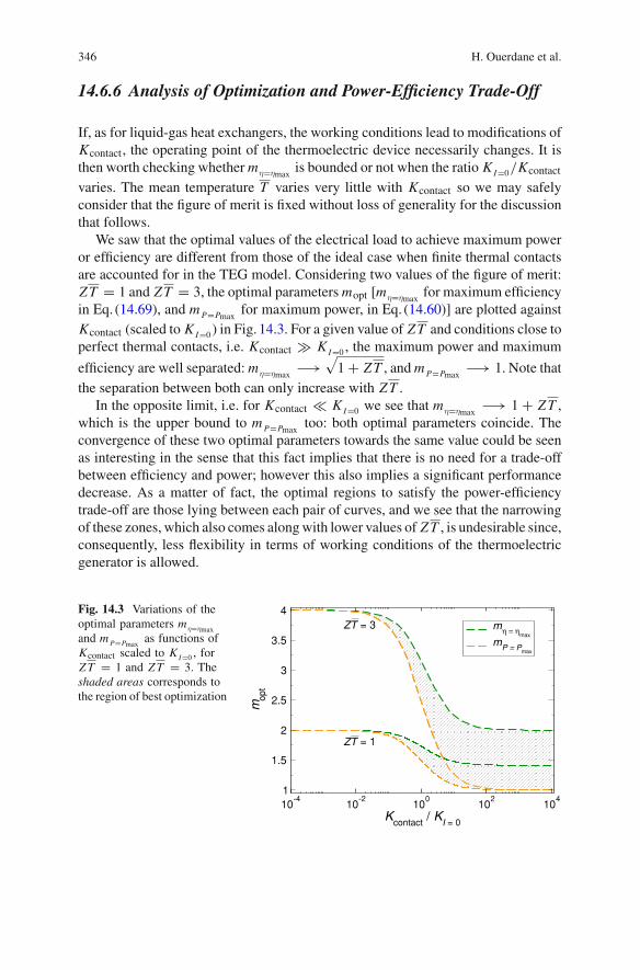
14.6.6 Analysis of Optimization and Power-Efficiency Trade-Off

If, as for liquid-gas heat exchangers, the working conditions lead to modifications ofKcontact, the operating point of the thermoelectric device necessarily changes. It isthen worth checking whether mη=ηmax

is bounded or not when the ratio KI=0/Kcontact

varies. The mean temperature T varies very little with Kcontact so we may safelyconsider that the figure of merit is fixed without loss of generality for the discussionthat follows.

We saw that the optimal values of the electrical load to achieve maximum poweror efficiency are different from those of the ideal case when finite thermal contactsare accounted for in the TEG model. Considering two values of the figure of merit:Z T = 1 and Z T = 3, the optimal parameters mopt [mη=ηmax

for maximum efficiencyin Eq. (14.69), and m P=Pmax

for maximum power, in Eq. (14.60)] are plotted againstKcontact (scaled to KI=0 ) in Fig. 14.3. For a given value of Z T and conditions close toperfect thermal contacts, i.e. Kcontact � KI=0 , the maximum power and maximum

efficiency are well separated: mη=ηmax−→

√1 + Z T , and m P=Pmax

−→ 1. Note thatthe separation between both can only increase with Z T .

In the opposite limit, i.e. for Kcontact � KI=0 we see that mη=ηmax−→ 1 + Z T ,

which is the upper bound to m P=Pmaxtoo: both optimal parameters coincide. The

convergence of these two optimal parameters towards the same value could be seenas interesting in the sense that this fact implies that there is no need for a trade-offbetween efficiency and power; however this also implies a significant performancedecrease. As a matter of fact, the optimal regions to satisfy the power-efficiencytrade-off are those lying between each pair of curves, and we see that the narrowingof these zones, which also comes alongwith lower values of Z T , is undesirable since,consequently, less flexibility in terms of working conditions of the thermoelectricgenerator is allowed.

Fig. 14.3 Variations of theoptimal parameters mη=ηmaxand m P=Pmax

as functions ofKcontact scaled to K I=0 , forZ T = 1 and Z T = 3. Theshaded areas corresponds tothe region of best optimization

10-4

10-2

100

102

104

Kcontact / KI = 0

1

1.5

2

2.5

3

3.5

4

mop

t

mη = ηmax

mP = Pmax

ZT = 3

ZT = 1


Fig. 14.4 Power versus effi-ciency curves for two caseswith a fixed figure of meritZ T = 1. Only the value ofKcontact varies

0 0.05 0.1 0.15 0.2 0.25 0.3 0.35efficiency

0

2

4

6

8

10

12

outp

ut p

ower

(ar

b. u

nit)

Kcontact = 50 KI = 0

Kcontact = 10 KI = 0

The Fig. 14.4 displays two power-efficiency curves, one for Kcontact = 10KI=0 ,the other for Kcontact = 50KI=0 . As the contact thermal conductance decreases, weobserve a narrowing of the optimal zone in accordance with our analysis of Fig. 14.3.The arrows indicate the maximal values that Pmax and ηmax may take. As the qualityof the thermal contacts deteriorates the power-efficiency curve reduces to a pointlocated at the origin.

14.7 Summary and Discussion on Efficiency at MaximumPower

Wepresented the force-flux formalism developed byOnsager [4, 5] and later adaptedto thermoelectricity by Callen [6] and Domenicali [7]. This formalism provides veryconvenient tools to obtain and analyze in simple terms the thermal and electricalconditionswhich allow themaximumpower productionbya thermoelectric generatornon-ideally coupled to heat reservoirs. These conditions are expressedvery simply forthe thermal impedance matching: the equality of the contact thermal conductancesand the equivalent thermal conductance of the TEG. It is crucial to see that thequality of the contacts between the TEG and the heat reservoirs is important sincehigh values of Z T are of limited interest otherwise. We also saw that the nontrivialinterplay between the thermal and electrical properties of the TEG makes difficultthe search for the optimum conditions for maximum output power production sinceboth electrical and thermal impedance matching must be satisfied simultaneously.Note that this is also the basic idea underlying the compatibility approach [25] forideal thermoelectric systems.

Searching for ways to increase the efficiency of thermoelectric conversionprocesses in devices operating in various environmental conditions boosts a varietyof research activities spanning from materials sciences to nonequilibrium statisticalmechanics at the mesoscale, and device modeling. All these areas of research are


highly topical. Approaches based on the concept of minimization of entropy pro-duction have been developed and proved successful in various sectors of thermalengineering and sciences [21]; new contributions continue to feed this field with,e.g., the recent introduction of the thermoelectric potential [16, 25, 26]. Since one isinterested in power rather than energy, thermoelectric efficiency has been analyzedin the frame of finite-time thermodynamics [27–30], focusing on the efficiency atmaximum power [31, 32]. Such efficiency was initially shown to be bounded bythe so-called formula of Curzon and Ahlborn (CA) in the specific case of endore-versible heat engines [20]. The analysis of Curzon and Ahlborn was later put onfirmer grounds in the frame of linear irreversible thermodynamics assuming a strongcoupling between the heat flux and the work [33] and further discussed by Apertet etal. [31, 32]. Analyses of efficiency at maximum power for nanoscopic quantum dotsystems [34] and extension to stochastic heat engines [35] are also being developed.

Thework presented in this Chapter and in research papers focusing on thermoelec-tric devices [31, 32, 36, 37] significantly advance the understanding of the centralconcept of energy conversion efficiency of heat engines. Since the advent of finitetime thermodynamics, the Curzon and Ahlborn efficiency has become a paradigm.Given the utmost importance of the physics of heat engines, which are ubiquitous inthe sense that they are systems useful to model biological cells, mesoscopic solid-state systems, macroscopic devices, we think that the CA efficiency, though wellestablished through the years, deserves close inspection. A very important work wasinitiated by Schmiedl and Seifert (SS), but the crucial question of the discrepancybetween their result and the CA efficiency remained without answers until now. Theanswer, far from trivial, required an in-depth analysis on the nature of irreversibilitiesin heat engines [31, 32]. If one overlooks some of the subtleties that we put forth,one may not succeed in providing a sound and clear framework that explains in atransparent fashion the energy conversion efficiency of heat engines. Our work, tosome extent, provides a shift in paradigm: we have come not only to propose cleardefinitions of both CA and SS efficiencies but also show that a systemmay undergo acontinuous transition from one type of efficiency to the other by tuning the differentsources of irreversibility. These facts are crucial for any optimization work.

14.8 Outlook on the Next Frontier: The Mesoscopic Scale

Mesoscopic systems offer an interesting field of play at the crossroads of quantumand classical physics, to experimentalists aswell as theoreticians. Indeed, the study ofmesoscopic systems cannot be reduced to practical work aiming only at miniaturiza-tion of transistors for microelectronics applications. From a fundamental viewpoint,it is in these systems that the size of fluctuations become sufficiently important ascompared to averages, so that their influence on the systems’ properties emerges. Theonset of quantum effects at the mesoscopic scale depends on the size of the consid-ered system, its temperature and external constraints that depend on the interactionswith its environment.


Over the last 30 years great strides were made in fabrication of artificial struc-tures down to very small scales. Operation of a number of modern devices rely ona proper understanding of the physics of nano- and mesoscale structures such as,e.g., semiconductor quantum wells, superlattices, and quantum dots, which todayare routinely produced as high quality custom-made samples. Mesoscopic systemsare characterized by a great number of constituents. For some applications or funda-mental studies involving conversion of transfer of energy, they can be considered asheat engines; so it is tempting to describe and analyze them using the concepts andterminology that derive from classical thermodynamics. As a matter of fact, suchnotions as, e.g., entropy and entropy production, which we saw in Sect. 14.2, mustbe revisited considering that mesoscopic devices operate in regimes far from equi-librium where fluctuations are strong. This implies that transport phenomena andthe related measurable quantities in these systems must be identified and understoodproperly.

The experimental study of electron transport, which is typically ballistic andcoherent in mesoscopic systems, can be performed with the so-called quantumpoint contacts (QPCs); these narrow, confining constrictions are made up betweenwider conducting regions of the system under consideration, and their width iscomparable to the electrons’ wavelength at low temperatures. The quantization ofballistic electron transport through such constriction demonstrates that conductionis transmission. Because of conductance quantization [38] in quantum point con-tacts, the Seebeck coefficient was analyzed at the threshold energies of the con-ductance plateaus, where the change in the conductance is very important. VanHouten et al. [39] obtained the Seebeck coefficient in a system based on QPC in atwo dimentional electronic gas of a GaAs-AlGaAs semiconducting heterostructures.They concluded that the thermopower exhibits quantum size effects and oscillateseach time a new mode opens up in the QPC.

For thermoelectric systems at this scale, this calls for the development of recentapproaches such as, e.g., finite time thermodynamics [27–30] and stochastic ther-modynamics [40–43], and their association to those which proved fruitful for thecomputation and measurement of the thermoelectric transport coefficients. TheLandauer-Buttiker formalism provides necessary tools to consider nano-systemsplaced between several reservoirs and study the multichannel scattering. Sivain andImry [44] used this approach to compute and study linear transport coefficients of athermoelectric sample characterized by some disorder in a case where the connec-tions to the chemical and temperature reservoirs are achievedwith ideal multichannelleads. Dissipation processes due to inelastic scattering were assumed to occur only inthe reservoirs. By looking at the thermopower near themobility edge, they pointed outsome deviations of the kinetic coefficients from Onsager’s relations and the Seebeckcoefficient from the Cutler-Mott formula.

More recentworks [45–47] challenge the view that thermoelectric heat engines areby nature irreversible in their operation. The purpose of these indeed is to find waysto allow reversible diffusive transport in thermoelectric materials and the proposedroute is that of nanostructures, which if they are sufficiently well tailored, permitthe narrowing of the charge carriers’ densities of states (DOS). The idea is that


if electron transport is limited to a narrow energy band which corresponds to anenergy such that the two Fermi functions characterizing the hot and cold reservoirsrespectively, are equal, then together with a weak electron-phonon, coupling, frictioneffects are drastically reduced. While delta-function may represent an ideal limit,quantum confinement effects generate a finite lower bound to the DOS widths, andhence limit the efficiency of the device.

Our view on the matter of irreversibility derives from the main message of finitetime thermodynamics: trading a part of the efficiency for the ability to produce poweris possible only if irreversible processes are introduced in the thermodynamic cycle.Further, using numerical simulations we demonstrated, in the case of a two thermallycoupled macroscopic heat engines, that efficiency at maximum power is increasedwhen the hot-side Joule heating is favoured [32]. We interpreted this result as arecycling of the degraded energy: if it is evacuated to the hot heat reservoir, thisenergy becomes available to be used again, while if it is evacuated to the cold side, itis irretrievably lost. These considerations must be examined at the mesoscale, whereirreversible thermodynamics has not completely given way to reversible dynamics.Finally, we showed that optimization of the operation of a TEGmust simultaneouslysatisfy electrical and thermal impedance matching. At the mesoscale the notion ofimpedance matching must be considered with care. Adaptation of our analysis tomesoscale thermal engines is underway, and we have every reason to be optimistic.

References

1. T.J. Seebeck, Abhandlungen Königliche Akademie der Wissenschaften zu Berlin, 289 (1821)2. J.C.A. Peltier, Annales de Chimie Physique 56, 371 (1834)3. H.B.Callen,Thermodynamics and an Introduction to Thermostatistics, 2nd revised edn. (Wiley,

1985)4. L. Onsager, Phys. Rev. 37, 405 (1931)5. L. Onsager, Phys. Rev. 38, 2265 (1931)6. H.B. Callen, Phys. Rev. 73, 1349 (1948)7. C.A. Domenicali, Rev. Mod. Phys. 26, 237 (1954)8. M. Le Bellac, F. Mortessagne, G.G. Batrouni, Equilibrium and Non-Equilibrium Statistical

Thermodynamics (Cambridge University Press, 2004)9. I. Prigogine, Introduction to Thermodynamics of Irreversible Processes, 3rd edn. (Wiley, New

York, 1968)10. N. Pottier, Physique Statisitique Hors équilibre, Processus Irréversibles Linéaires (EDP Sci-

ences/CNRS Editions, Paris, 2007)11. Y. Rocard, Thermodynamique, 2nd edn. (Masson, Paris, 1967)12. H.B. Callen, T.A. Welton, Phys. Rev. 83, 34 (1951)13. R. Kubo, Rep. Prog. Phys. 29, 255 (1966)14. A. Ioffe, Semiconductor Thermoelements and Thermoelectric Cooling (Infosearch, ltd., Lon-

don, 1957)15. Y. Apertet, H. Ouerdane, C. Goupil, P. Lecoeur, J. Phys. Conf. Series 395, 012203 (2012)16. C. Goupil, W. Seifert, K. Zabrocki, E. Müller, G.J. Snyder, Entropy 13, 1481 (2011)17. M. Freunek, M. Müller, T. Ungan, W. Walker, L.M. Reindl, J. Electron. Mat. 38, 1214 (2009)18. P. Chambadal, Les Centrales Nucléaires (Armand Colin, 1957)19. I.I. Novikov, J. Nucl. En. 7, 125 (1958)


20. F. Curzon, B. Ahlborn, Am. J. Phys 43, 22 (1975)21. A. Bejan, J. Appl. Phys. 79, 1191 (1996)22. J.W. Stevens, En. Conv. Manag. 42, 709 (2001)23. K. Yasawa, A. Shakouri, Environ. Sci. Technol. 45, 7548 (2011)24. D. Nemir, J. Beck, J. Electon. Mat 39, 1897 (2010)25. G.J. Snyder, T.S. Ursell, Phys. Rev. Lett. 91, 148301 (2003)26. C. Goupil, J. Appl. Phys. 106, 104907 (2009)27. B. Andresen, P. Salamon, R.S. Berry, J. Chem. Phys. 66, 1571 (1977)28. B. Andresen, R.S. Berry, A. Nitzan, P. Salamon, Phys. Rev. A 15, 2086 (1977)29. P. Salamon, B. Andresen, R.S. Berry, Phys. Rev. A 15, 2094 (1977)30. B. Andresen, Angew. Chem. Int. Ed. 50, 2690 (2011)31. Y. Apertet, H. Ouerdane, C. Goupil, P. Lecoeur, Phys. Rev. E 85, 031116 (2012)32. Y. Apertet, H. Ouerdane, C. Goupil, P. Lecoeur, Phys. Rev. E 85, 041144 (2012)33. C. Van den Broeck, Phys. Rev. Lett. 95, 190602 (2005)34. M. Esposito, K. Lindenberg, C. Van den Broeck, Europhys. Lett. 85, 60010 (2009)35. T. Schmiedl, U. Seifert, Europhys. Lett. 81, 20003 (2008)36. Y. Apertet, H. Ouerdane, O. Glavatskaya, C. Goupil, P. Lecoeur, Europhys. Lett. 97, 28001

(2012)37. Y. Apertet, H. Ouerdane, C. Goupil, P. Lecoeur, Phys. Rev. B 85, 033201 (2012)38. B.J. Van Wees et al., Phys. Rev. Lett. 60, 848 (1988)39. H. Van Houten, L.W. Molenkamp, C.W.J. Beenakker, C.T. Foxon, Semicond. Sci. Technol. B

215, 7 (1992)40. C. Van den Broeck, Stochastic Thermodynamics (Springer, 1986)41. U. Seifert, Eur. Phys. J. B 64, 423 (2008)42. K. Sekimoto, Stochastic Energetics (Springer, 2010)43. M. Esposito, Phys. Rev. E 85, 041125 (2012)44. U. Sivain, Y. Imry, Phys. Rev. B 33, 551 (1986)45. T.E. Humphrey, H. Linke, Phys. Rev. Lett. 94, 096601 (2005)46. N. Nakpathomkun, H.Q. Xu, H. Linke, Phys. Rev. B 82, 235428 (2010)47. O. Karlström, H. Linke, G. Karlström, A. Wacker, Phys. Rev. B 84, 113415 (2011)

chapter 14 a linear nonequilibrium thermodynamics approach ... · 14 a linear nonequilibrium...

Documents