CHAPTER 14Comparing two groups

Dr Richard Bußmann

COMPARING PERFORMANCES

• Do customers spend more using their credit card if they are given an incentive such as “double miles” or “double coupons” toward flights, hotel stays, or store purchases?

• To answer questions such as this, credit card issuers often perform experiments on a sample of customers, making them an offer of an incentive, while other customers receive no offer.

• By comparing the performance of the two offers on the sample, they can decide whether the new offer would provide enough potential profit if they were to “roll it out” and offer it to their entire customer base.

COMPARING TWO MEANS

• The statistic of interest is the difference in the observed means of the offer and no offer groups:

• What we’d really like to know is the difference of the means in the population at large:

• Now the population model parameter of interest is the difference between the means.

COMPARING TWO MEANS

• In order to tell if a difference, that we observe in the sample means, indicates a real difference in the underlying population means, we’ll need to know the sampling distribution model and standard deviation of the difference.

• Once we know those, we can build a confidence interval and test a hypothesis, just as we did for a single mean.

COMPARING TWO MEANS

• It’s easy to find the mean and standard deviation of the spend lift (increase in spending) for each of these groups, but that’s not what we want.

• We need the standard deviation of the difference in their means.

• For that, we can use a simple rule: • If the sample means come from independent samples, the

variance of their sum or difference is the sum of their variances.

COMPARING TWO MEANS

• As long as the two groups are independent, we find the standard deviation of the difference between the two sample means by adding their variances and then taking the square root:

COMPARING TWO MEANS

• Usually we don’t know the true standard deviations of the two groups, and , so we substitute the estimates, and , and find a standard error:

• We’ll use the standard error to see how big the difference really is.

COMPARING TWO MEANS

• Just as for a single mean, the ratio of the difference in the means to the standard error of that difference has a sampling model that follows a Student’s t distribution.

• The sampling model isn’t really Student’s t, but by using a special, adjusted degrees of freedom value, we can find a Student’s t-model that is so close to the right sampling distribution model that nobody can tell the difference.

• Since it doesn’t help our understanding, we leave it to the computer or calculator.

• We can model the standardized sample difference between the means of two independent groups with a Student’s t-model

COMPARING TWO MEANS

TWO SAMPLE T-TEST

• To construct the hypothesis test for the difference of the means, we start by hypothesizing a value for the true difference of the means. We’ll call that hypothesized difference .

• It’s so common for that hypothesized difference to be zero that we often just assume

TWO SAMPLE T-TEST

• The two-sample t-test is the ratio of the difference in the means from our samples to its standard error compared to a critical value from a Student’s t-model.

• Hence

• Assuming

• So

• When the null holds, the statistic can be modelled by a Student’s t-model with df given by a special formula.

• The t-ratio (p-value) can then be compared with a

ASSUMPTIONS & CONDITIONS

• Independence Assumption• The data in each group must be drawn independently and at

random from each group’s own homogeneous population or generated by a randomized comparative experiment.

• Randomization Condition• Without randomization of some sort, there are no sampling

distribution models and no inference.

• 10% Condition• We usually don’t check this condition for differences of

means. We needn’t worry about it at all for randomized experiments.

ASSUMPTIONS & CONDITIONS

• Normal Population Assumption• We need the assumption that the underlying populations are

each Normally distributed.

• Nearly Normal Condition• We must check this for both groups; a violation by either one

violates the condition.

• Independent Groups Assumption• To use the two-sample t methods, the two groups we are

comparing must be independent of each other. • No statistical test can verify that the groups are independent.

You have to think about how the data were collected.

• A hypothesis test really says nothing about the size of the difference. All it says is that the observed difference is large enough that we can be confident it isn’t zero.

• Given the conditions and assumptions, a two-sample t-interval for the difference between means and is found using the critical value , given the df and a confidence level.

• Hence the confidence interval becomes

CONFIDENCE INTERVAL FOR THE DIFFERENCE BETWEEN TWO MEANS

EXAMPLE

• A market analyst wants to know if a new website is showing increased page views per visit. A customer is randomly sent to one of two different websites, offering the same products, but with different designs. Given statistics below, find the estimated mean difference in page visits between the two websites.

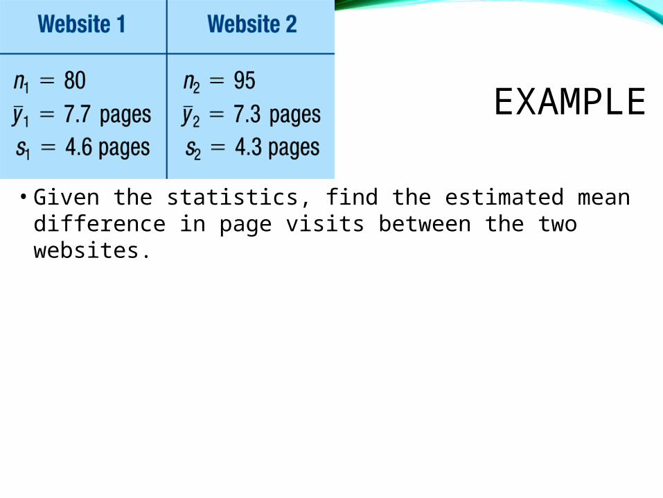
• Given the statistics, find the estimated mean difference in page visits between the two websites.

EXAMPLE

EXAMPLE

• A market analyst wants to know if a new website is showing increased page views per visit. A customer is randomly sent to one of two different websites, offering the same products, but with different designs.

• What does the confidence interval [–0.938, 1,738] say about the null hypothesis that the mean difference in page views from the two websites?

EXAMPLE

• A market analyst wants to know if a new website is showing increased page views per visit. A customer is randomly sent to one of two different websites, offering the same products, but with different designs.

• What does the confidence interval [–0.938, 1,738] say about the null hypothesis that the mean difference in page views from the two websites?

• Fail to reject the null hypothesis. Since 0 is in the interval, it is a plausible value for the true difference in means.

EXAMPLE

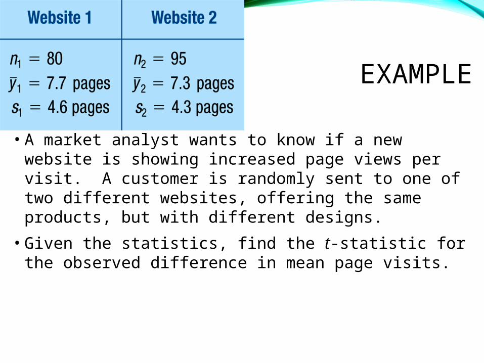
• A market analyst wants to know if a new website is showing increased page views per visit. A customer is randomly sent to one of two different websites, offering the same products, but with different designs.

• Given the statistics, find the t-statistic for the observed difference in mean page visits.

EXAMPLE• A market analyst wants to know if a new website is

showing increased page views per visit. A customer is randomly sent to one of two different websites, offering the same products, but with different designs.

• What does the hypothesis test results, t = 0.59 and p–value = 0.5557 say about the null hypothesis that the mean difference in page views from the two websites?

• Fail to reject the null hypothesis. There is insufficient evidence to conclude a statistically significant mean difference in the number of webpage visits.

• Is this consistent with the conclusion drawn from the confidence interval?

• Yes, the conclusion is the same.

POOLED T-TEST

• If you bought a used camera in good condition from a friend, would you pay the same as you would if you bought the same item from a stranger?

• One group of people in an experiment was told to imagine buying from a friend whom they expected to see again.

• The other group was told to imagine buying from a stranger.

POOLED T-TEST

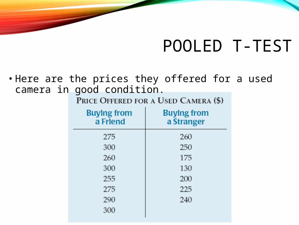
• Here are the prices they offered for a used camera in good condition.

POOLED T-TEST

• The usual null hypothesis is that there’s no difference in means and that’s what we’ll use for the camera purchase prices.

• When we performed the t-test earlier in the chapter, we used an approximation formula that adjusts the degrees of freedom to a lower value.

• When is only 15, as it is here, we don’t really want to lose any degrees of freedom.

POOLED T-TEST

• If we’re willing to assume that the variances of the groups are equal (at least when the null hypothesis is true), then we can save some degrees of freedom.

• To do that, we have to pool the two variances that we estimate from the groups into one common, or pooled, estimate of the variance:

POOLED T-TEST

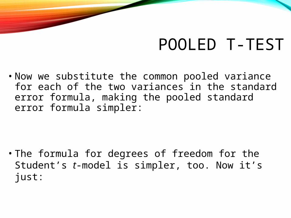
• Now we substitute the common pooled variance for each of the two variances in the standard error formula, making the pooled standard error formula simpler:

• The formula for degrees of freedom for the Student’s t-model is simpler, too. Now it’s just:

EQUAL VARIANCE ASSUMPTION

• To use the pooled t-methods, you’ll need to add the Equal Variance Assumption that the variances of the two populations from which the samples have been drawn are equal.

• That is

• The remaining conditions are the same as for the two sample t-test.

POOLED T-TEST

• We then test the hypothesis

With

Using

POOLED T-TEST

• Where

• And

• If the conditions and asssumtions hold, then the statistics sampling distribution can be modelled with a Student’s t-model with

POOLED T-TEST

• This gives the pooled-t confidence interval of

• With

• that depends on the confidence level and degrees of freedom of

WHEN TO USE A POOLED T-TEST

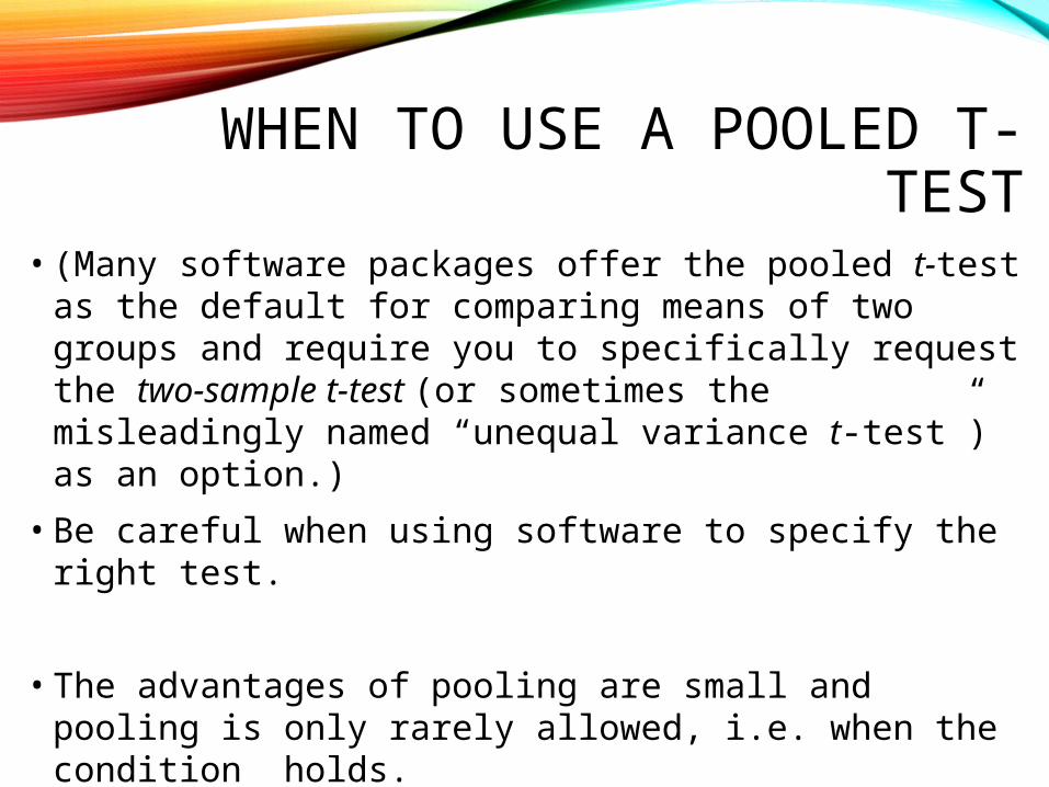
• (Many software packages offer the pooled t-test as the default for comparing means of two groups and require you to specifically request the two-sample t-test (or sometimes the misleadingly named “unequal variance t-test”) as an option.)

• Be careful when using software to specify the right test.

• The advantages of pooling are small and pooling is only rarely allowed, i.e. when the condition holds.

• As it’s also never wrong not to pool, just don’t pool…

TURKEY’S QUICK TEST

• To use Tukey’s test, one group must have the highest value, and the other must have the lowest.

• We count how many values in the high group are higher than all the values of the lower group.

• Add to this the number of values in the low group that are lower than all the values of the higher group.

• You can count ties as ½.

TURKEY’S QUICK TEST

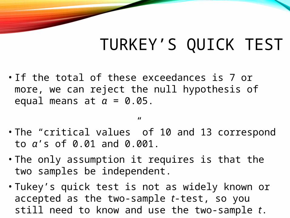
• If the total of these exceedances is 7 or more, we can reject the null hypothesis of equal means at α = 0.05.

• The “critical values” of 10 and 13 correspond to α’s of 0.01 and 0.001.

• The only assumption it requires is that the two samples be independent.

• Tukey’s quick test is not as widely known or accepted as the two-sample t-test, so you still need to know and use the two-sample t.

© 2010 Pearson Education

PAIRED DATA

• The independence assumption for the two-sample t-test is crucial.

• However, quite commonly, we have data on the same cases in two different circumstances. Data such as these are called paired.

• Paired data commonly occur as “before and after” measurements of some property.

• Note: You should not use the two-sample (or pooled two-sample) method when the data are paired.

PAIRED DATA

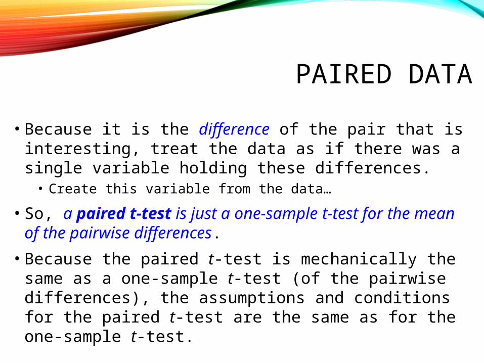
• Because it is the difference of the pair that is interesting, treat the data as if there was a single variable holding these differences.• Create this variable from the data…

• So, a paired t-test is just a one-sample t-test for the mean of the pairwise differences.

• Because the paired t-test is mechanically the same as a one-sample t-test (of the pairwise differences), the assumptions and conditions for the paired t-test are the same as for the one-sample t-test.

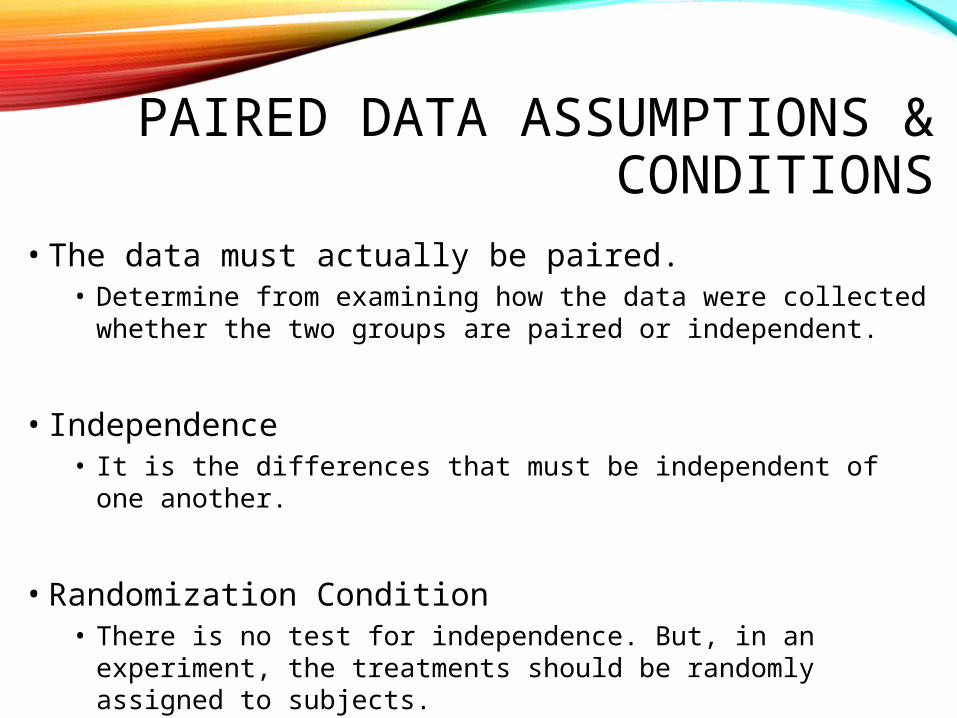
PAIRED DATA ASSUMPTIONS & CONDITIONS

• The data must actually be paired.• Determine from examining how the data were collected

whether the two groups are paired or independent.

• Independence• It is the differences that must be independent of one another.

• Randomization Condition• There is no test for independence. But, in an experiment, the

treatments should be randomly assigned to subjects.

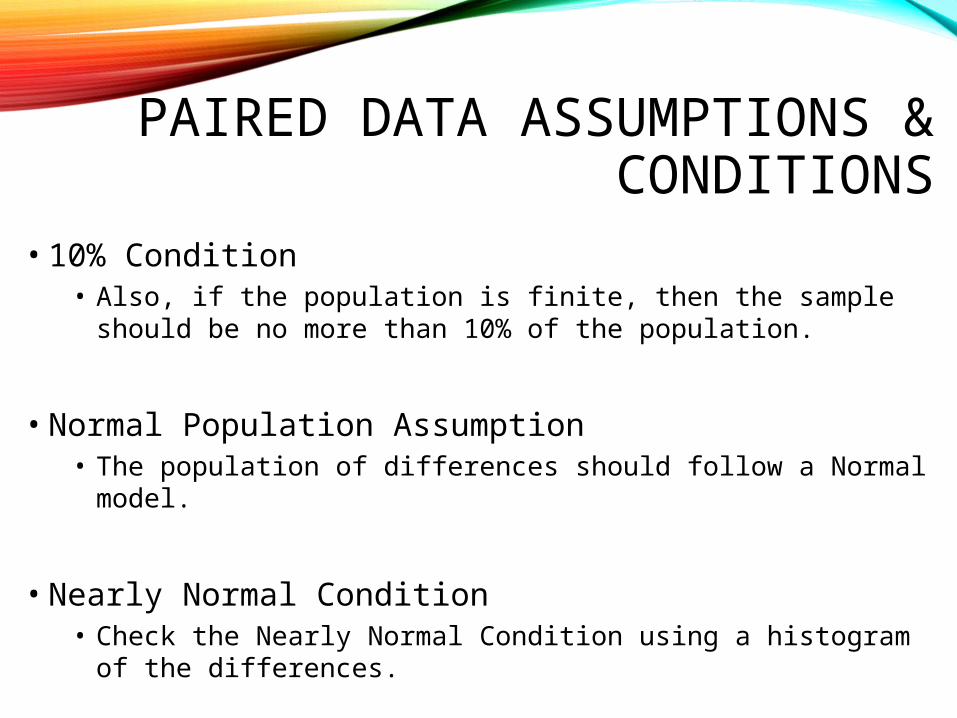
PAIRED DATA ASSUMPTIONS & CONDITIONS

• 10% Condition• Also, if the population is finite, then the sample should be no

more than 10% of the population.

• Normal Population Assumption• The population of differences should follow a Normal model.

• Nearly Normal Condition• Check the Nearly Normal Condition using a histogram of the

differences.

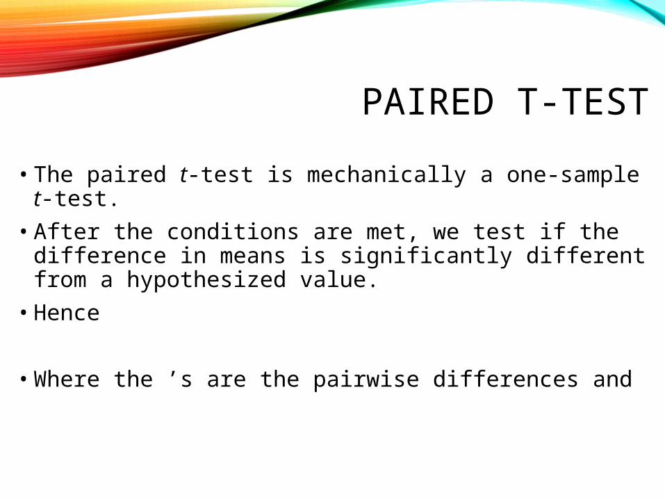
PAIRED T-TEST

• The paired t-test is mechanically a one-sample t-test.

• After the conditions are met, we test if the difference in means is significantly different from a hypothesized value.

• Hence

• Where the ’s are the pairwise differences and

PAIRED T-TEST

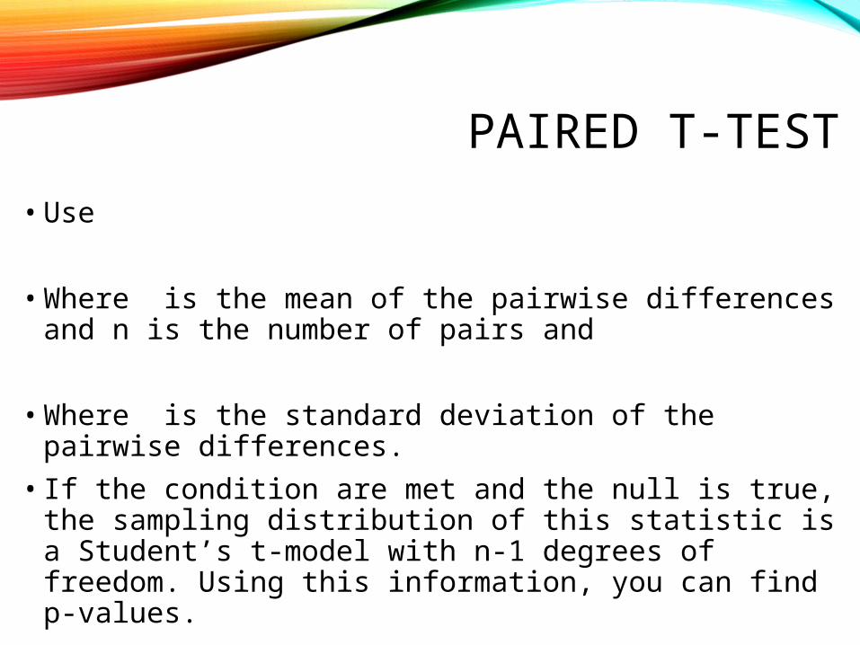
• Use

• Where is the mean of the pairwise differences and n is the number of pairs and

• Where is the standard deviation of the pairwise differences.

• If the condition are met and the null is true, the sampling distribution of this statistic is a Student’s t-model with n-1 degrees of freedom. Using this information, you can find p-values.

PAIRED T-TEST

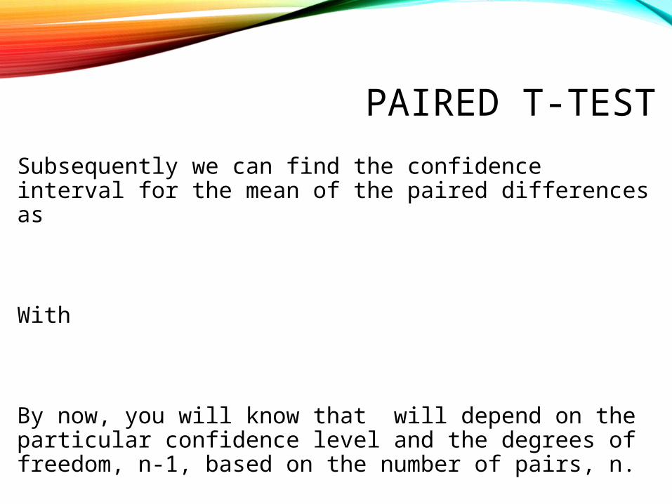
Subsequently we can find the confidence interval for the mean of the paired differences as

With

By now, you will know that will depend on the particular confidence level and the degrees of freedom, n-1, based on the number of pairs, n.

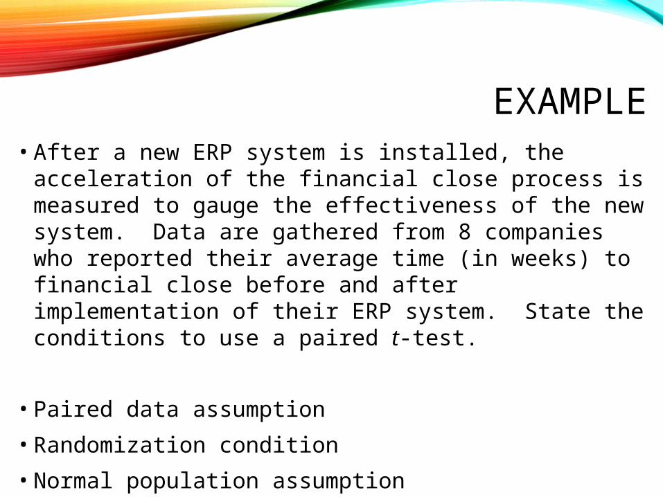
EXAMPLE• After a new ERP system is installed, the acceleration of

the financial close process is measured to gauge the effectiveness of the new system. Data are gathered from 8 companies who reported their average time (in weeks) to financial close before and after implementation of their ERP system. State the conditions to use a paired t-test.

• Paired data assumption

• Randomization condition

• Normal population assumption

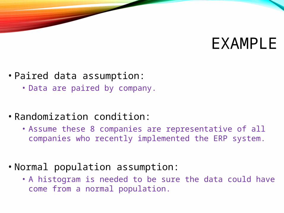
EXAMPLE

• Paired data assumption: • Data are paired by company.

• Randomization condition: • Assume these 8 companies are representative of all

companies who recently implemented the ERP system.

• Normal population assumption: • A histogram is needed to be sure the data could have come

from a normal population.

EXAMPLE

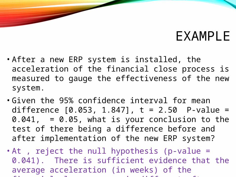
• After a new ERP system is installed, the acceleration of the financial close process is measured to gauge the effectiveness of the new system.

• Given the 95% confidence interval for mean difference [0.053, 1.847], t = 2.50 P-value = 0.041, = 0.05, what is your conclusion to the test of there being a difference before and after implementation of the new ERP system?

• At , reject the null hypothesis (p-value = 0.041). There is sufficient evidence that the average acceleration (in weeks) of the financial close process is different after implementation of a new ERP system.

CAUTION

• Watch out for paired data when using the two-sample t-test.

• Don’t use individual confidence intervals for each group to test the difference between their means.

• Look at the plots.

• Don’t use a paired t-method when the samples aren’t paired.

• Don’t forget to look for outliers when using paired methods.

SUMMARY

• Know how to test whether the difference in the means of two independent groups is equal to some hypothesized value.

• The two-sample t-test is appropriate for independent groups. It uses a special formula for degrees of freedom.

• The Assumptions and Conditions are the same as for one-sample inferences for means with the addition of assuming that the groups are independent of each other.

• The most common null hypothesis is that the means are equal.

SUMMARY

• Be able to construct and interpret a confidence interval for the difference between the means of two independent groups.

• The confidence interval inverts the t-test in the natural way.

• Know how and when to use pooled t inference methods.

• There is an additional assumption that the variances of the two groups are equal.

• This may be a plausible assumption in a randomized experiment.

SUMMARY

• Recognize when you have paired or matched samples and use an appropriate inference method.

• Paired t methods are the same as one-sample t methods applied to the pairwise differences.

• If data are paired they cannot be independent, so two-sample t and pooled-t methods would not be applicable.

SUMMARY

• The standard error for the difference in sample means relies on the assumption that our data come from independent groups. • Pooling is usually not the best choice here.

• We can add variances of independent random variables to find the standard deviation of the difference in two independent means.