chapter 14 equilibrium and efficiency copyright © 2014 mcgraw-hill education. all rights reserved....
TRANSCRIPT

chapter 14
Equilibrium and Efficiency
Copyright © 2014 McGraw-Hill Education. All rights reserved. No reproduction or distribution without the prior written consent of McGraw-Hill Education.
14-2
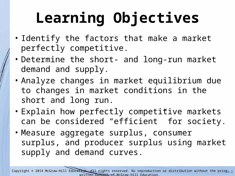
Learning Objectives• Identify the factors that make a market perfectly
competitive.• Determine the short- and long-run market demand
and supply.• Analyze changes in market equilibrium due to changes
in market conditions in the short and long run.• Explain how perfectly competitive markets can be
considered “efficient” for society.• Measure aggregate surplus, consumer surplus, and
producer surplus using market supply and demand curves.
Copyright © 2014 McGraw-Hill Education. All rights reserved. No reproduction or distribution without the prior written consent of McGraw-Hill Education.

14-3
Overview
• What makes a market competitive, so that individuals and firms behave as price takers?
• We will aggregate the individual demand and supply curves we already know into market demand and supply curves
• We will analyze the short-run and long-run dynamics and equilibria of competitive markets
• We will show that the equilibrium outcome in competitive markets is efficient, maximizing aggregate surplus
Copyright © 2014 McGraw-Hill Education. All rights reserved. No reproduction or distribution without the prior written consent of McGraw-Hill Education.

14-4
Characteristics of a Perfectly Competitive Market
1. Buyers and sellers face no transaction costs2. Products are homogeneous, identical in the eyes of
the consumer3. There are many buyers and sellers, each accounting
for a small fraction of the overall demand or supply of the good
4. In a perfectly competitive market, buyers and sellers are price takers, taking the market price as given (unaffected by their actions) in deciding how much to buy or sell
Copyright © 2014 McGraw-Hill Education. All rights reserved. No reproduction or distribution without the prior written consent of McGraw-Hill Education.

14-5
Market Demand
• Market demand: sum of the demands of all the individual consumers
• Market demand curve: horizontal sum of the individual demand curves
Copyright © 2014 McGraw-Hill Education. All rights reserved. No reproduction or distribution without the prior written consent of McGraw-Hill Education.

14-6
Individual and Market Demand Curves
E
J
E J+
Copyright © 2014 McGraw-Hill Education. All rights reserved. No reproduction or distribution without the prior written consent of McGraw-Hill Education.

14-7
Market Supply
• Market supply: sum of the supply of all the individual sellers
• Market supply curve: horizontal sum of the individual supply curves
Copyright © 2014 McGraw-Hill Education. All rights reserved. No reproduction or distribution without the prior written consent of McGraw-Hill Education.

14-8
Individual and Market Supply Curves
A A R
R
+
Copyright © 2014 McGraw-Hill Education. All rights reserved. No reproduction or distribution without the prior written consent of McGraw-Hill Education.

14-9
Short-Run vs. Long-Run Market Supply
• Market supply curves– Short-run supply: Add up the short-run supply
curves of all currently active firms– Long-run supply: Add up the long-run supply
curves of all potential suppliers
Copyright © 2014 McGraw-Hill Education. All rights reserved. No reproduction or distribution without the prior written consent of McGraw-Hill Education.

The Long -Run Market Supply Curve with Free Entry
Free entry: when technology is freely available to anyone who wishes to start a firm, and entry is unrestricted. In that case, the number of potential firms is unlimited.
14-10Copyright © 2014 McGraw-Hill Education. All rights reserved. No reproduction or distribution without the prior written consent of McGraw-Hill Education.

14-11
Competitive Equilibrium
Copyright © 2014 McGraw-Hill Education. All rights reserved. No reproduction or distribution without the prior written consent of McGraw-Hill Education.
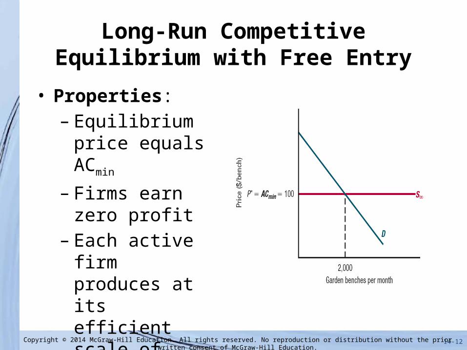
Long-Run Competitive Equilibrium with Free Entry
• Properties:– Equilibrium price
equals ACmin
– Firms earn zero profit
– Each active firm produces at its efficient scale of production
14-12Copyright © 2014 McGraw-Hill Education. All rights reserved. No reproduction or distribution without the prior written consent of McGraw-Hill Education.

14-13
D’
S10
AS∞
D
Garden benches per month
Pric
e ($
/ben
ch)
2,000
P*= ACmin
= 100
(b) Demand decrease
C
1,000
Short-Run and Long-Run Responses to Demand Change
Garden benches per month
Pric
e ($
/ben
ch)
2,000
A
D’D
S∞P*= ACmin
= 100
(a) Demand increase
4,000
C
S10
B
QSR
PSR
BPSR
QSR
Copyright © 2014 McGraw-Hill Education. All rights reserved. No reproduction or distribution without the prior written consent of McGraw-Hill Education.

14-14
Price Changes in the Long-Run
Garden benches per month2,000
Pric
e ($
/ben
ch)
(a) Increasing input cost
AACmin= 100
S∞
DD’ D’
S10
ACmin= 110 Ŝ∞
ACmin= 90Ŝ∞
4,000
C
S10
A
Garden benches per month2,000
Pric
e ($
/ben
ch)
(b) Decreasing input cost
ACmin= 100
S∞
D
4,000
C
B
E
QLR
E
QLR
B
Copyright © 2014 McGraw-Hill Education. All rights reserved. No reproduction or distribution without the prior written consent of McGraw-Hill Education.

14-15
Aggregate Surplus
• Aggregate surplus: captures the net benefit created by the production and consumption of a good
• Aggregate surplus = Total benefit from consumption (total
willingness to pay) – Total avoidable cost of production
Copyright © 2014 McGraw-Hill Education. All rights reserved. No reproduction or distribution without the prior written consent of McGraw-Hill Education.
14-16
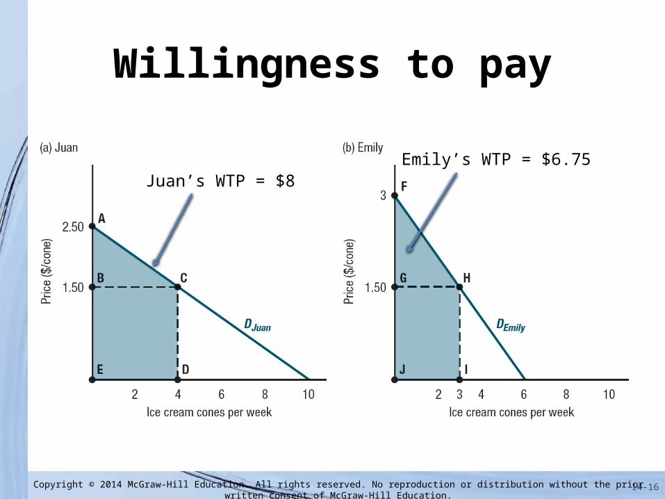
Willingness to pay
Juan’s WTP = $8Emily’s WTP = $6.75
Copyright © 2014 McGraw-Hill Education. All rights reserved. No reproduction or distribution without the prior written consent of McGraw-Hill Education.

14-17
Avoidable Cost of Production
Anitra’s ACP = $5
Robert’s ACP = $3
Copyright © 2014 McGraw-Hill Education. All rights reserved. No reproduction or distribution without the prior written consent of McGraw-Hill Education.

14-18
Competitive Equilibrium Maximizes Aggregate Surplus
• Pareto efficient (or Pareto optimal): an economic outcome at which it is impossible to make anyone better off without making someone else worse off
• Any change in who consumes the good, which firms produce it, or the amount that is produced and consumed, must lower aggregate surplus, making someone worse off in the process
Copyright © 2014 McGraw-Hill Education. All rights reserved. No reproduction or distribution without the prior written consent of McGraw-Hill Education.

Effects of Change in Who Consumes Good
Transferring one ice cream cone from Juan to Emily results in lower aggregate surplus (Juan’s WTP(3) > Emily’s WTP(4))
14-19Copyright © 2014 McGraw-Hill Education. All rights reserved. No reproduction or distribution without the prior written consent of McGraw-Hill Education.

Effects of Change in Who Produces Good
Transferring production of one ice cream cone from Anitra to Robert results in lower aggregate surplus (Anitra’s ACP(3) < Robert’s ACP(4))
14-20Copyright © 2014 McGraw-Hill Education. All rights reserved. No reproduction or distribution without the prior written consent of McGraw-Hill Education.

Effects of an Increase in Goods Produced and Consumed
Robert’s cost of producing an additional ice cream cone exceeds Juan’s willingness to pay for that ice cream cone, lowering aggregate surplus
14-21Copyright © 2014 McGraw-Hill Education. All rights reserved. No reproduction or distribution without the prior written consent of McGraw-Hill Education.

Using Market Demand as a Measure of Willingness to Pay
• Whenever the units of a good are consumed by those individuals with the highest willingness to pay for them, we can measure consumers’ total willingness to pay for the units they consume by the area under the market demand curve up to that quantity.
14-22Copyright © 2014 McGraw-Hill Education. All rights reserved. No reproduction or distribution without the prior written consent of McGraw-Hill Education.

Using Supply Curves to Measure Total Avoidable Cost
• Whenever the units of a good are produced by the firms with the lowest avoidable cost of producing them, we can measure firms’ total avoidable cost for the units they produce by the area under the market supply curve up to that quantity.
14-23Copyright © 2014 McGraw-Hill Education. All rights reserved. No reproduction or distribution without the prior written consent of McGraw-Hill Education.

Measuring Consumer and Producer Surplus
14-24Copyright © 2014 McGraw-Hill Education. All rights reserved. No reproduction or distribution without the prior written consent of McGraw-Hill Education.

Deadweight Loss• Deadweight Loss: a reduction in aggregate surplus
below its maximum possible valueCompetitive equilibrium:
- Maximum surplus- Zero DWL
14-25Copyright © 2014 McGraw-Hill Education. All rights reserved. No reproduction or distribution without the prior written consent of McGraw-Hill Education.

14-26
Consumer and Producer Surplus
• Consumer surplus: sum of consumers’ total willingness to pay minus their total expenditure
• Producer surplus: sum of firms’ revenue minus their avoidable costs
• Aggregate surplus = Consumer surplus + Producer surplus
Copyright © 2014 McGraw-Hill Education. All rights reserved. No reproduction or distribution without the prior written consent of McGraw-Hill Education.

14-27
Review
• A market is perfectly competitive when buyers and sellers face no transaction costs, products are homogeneous, and there are many buyers and sellers.
• In a long-run competitive equilibrium with free entry the equilibrium price equals ACmin, firms earn zero profit, and each active firm produces at its efficient scale of production.
• Aggregate surplus equals the sum of consumer surplus and producer surplus
• Competitive markets are Pareto efficient, maximizing aggregate surplus
Copyright © 2014 McGraw-Hill Education. All rights reserved. No reproduction or distribution without the prior written consent of McGraw-Hill Education.
14-28
Looking Forward
• Today we focused on competitive markets and how they maximize aggregate surplus
• Next we will analyze what happens when governments intervene in competitive markets using taxes, subsidies, price controls, tariffs, or other types of market intervention
Copyright © 2014 McGraw-Hill Education. All rights reserved. No reproduction or distribution without the prior written consent of McGraw-Hill Education.