chapter 16 general competitive equilibrium copyright ©2002 by south-western, a division of thomson...

Chapter 16

GENERAL COMPETITIVE EQUILIBRIUM

Copyright ©2002 by South-Western, a division of Thomson Learning. All rights reserved.

MICROECONOMIC THEORYBASIC PRINCIPLES AND EXTENSIONS

EIGHTH EDITION

WALTER NICHOLSON

Perfectly CompetitivePrice System

• We will assume that all markets are perfectly competitive– There is some number of homogeneous

goods in the economy• both consumption goods and factors of

production

– Each good has an equilibrium price– There are no transaction or transportation

costs– Everyone has perfect information

Law of One Price• A homogeneous good trades at the

same price no matter who buys it or who sells it– if one good traded at two different prices,

demanders would rush to buy the good where it was cheaper and firms would try to sell their output where the price was higher

• these actions would tend to equalize the price of the good

Assumptions of Perfect Competition

• There are a large number of people buying any one good– each person takes all prices as given– each person seeks to maximize utility given

his budget constraint

• There are a large number of firms producing each good– each firm attempts to maximize profits– each firm takes all prices as given

General Equilibrium

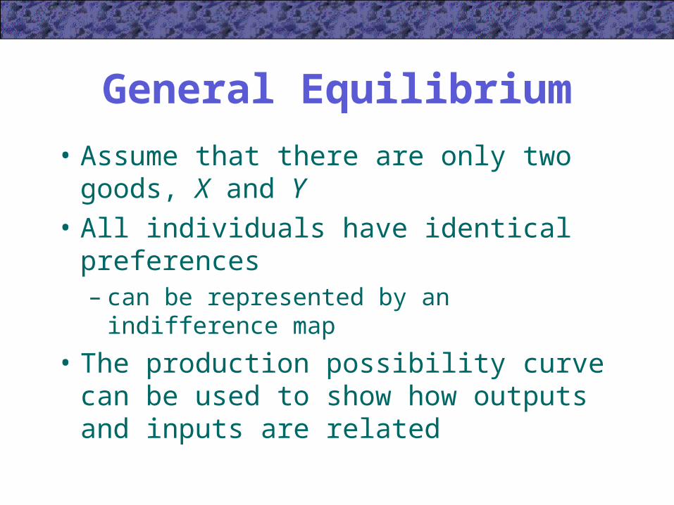
• Assume that there are only two goods, X and Y

• All individuals have identical preferences– can be represented by an indifference map

• The production possibility curve can be used to show how outputs and inputs are related

Edgeworth Box Diagram• Construction of the production possibility

curve for X and Y starts with the assumption that the amounts of K and L are fixed

• An Edgeworth box shows every possible way the existing K and L might be used to produce X and Y– Any point in the box represents a fully

employed allocation of the available resources to X and Y

Edgeworth Box Diagram

OX

OY

Total Labor

To

tal C

apit

al

A

Cap

ital

fo

r X

Cap

ital

fo

r Y

Labor for YLabor for X Capitalin Yproduction

Capitalin Xproduction

Labor in Y production

Labor in X production


• Many of the allocations in the Edgeworth box are inefficient– it is possible to produce more X and more Y

by shifting capital and labor around

• We will assume that competitive markets will not exhibit inefficient input choices

• We want to find the efficient allocations– they illustrate the actual production outcomes


• We will use isoquant maps for the two goods– the isoquant map for good X uses OX as the

origin

– the isoquant map for good Y uses OY as the origin

• The efficient allocations will occur where the isoquants are tangent to one another


OX

OY

Total Labor

To

tal C

apit

al

X2

X1

Y1

Y2

A

Point A is inefficient because, by moving along Y1, we can increaseX from X1 to X2 while holding Y constant


OX

OY

Total Labor

To

tal C

apit

al

X2

X1

Y1

Y2

A

We could also increase Y from Y1 to Y2 while holding X constantby moving along X1


OX

OY

Total Labor

To

tal C

apit

alAt each efficient point, the RTS (of K for L) is equal in bothX and Y production

X2

X1

X4

X3

Y1

Y2

Y3

Y4

P4

P3

P2

P1

Production Possibility Frontier

• The locus of efficient points shows the maximum output of Y that can be produced for any level of X– we can use this information to construct a

production possibility frontier• shows the alternative outputs of X and Y that

can be produced with the fixed capital and labor inputs

Production Possibility Frontier

Quantity of X

Quantity of Y

P4

P3

P2

P1

Y1

Y2

Y3

Y4

X1 X2 X3 X4

OX

OY

Each efficient point of productionbecomes a point on the productionpossibility frontier

The negative of the slope ofthe production possibilityfrontier is the rate of producttransformation (RPT)

Rate of Product Transformation

• The rate of product transformation (RPT) between two outputs is the negative of the slope of the production possibility frontier

frontiery possibilit production of slope ) for (of YXRPT

) (along ) for (of YXOOdX

dYYXRPT

Rate of Product Transformation

• The rate of product transformation shows how X can be technically traded for Y while continuing to keep the available productive inputs efficiently employed

Shape of the Production Possibility Frontier

• The production possibility frontier shown earlier exhibited an increasing RPT– this concave shape will characterize most

production situations

• RPT is equal to the ratio of MCX to MCY


• As production of X rises and production of Y falls, the ratio of MCX to MCY rises

– this occurs if both goods are produced under diminishing returns

• increasing the production of X raises MCX, while reducing the production of Y lowers MCY

– this could also occur if some inputs were more suited for X production than for Y production


• But we have assumed that inputs are homogeneous

• We need an explanation that allows homogeneous inputs and constant returns to scale

• The production possibility frontier will be concave if goods X and Y use inputs in different proportions

Opportunity Cost• The production possibility frontier

demonstrates that there are many possible efficient combinations of two goods

• Producing more of one good necessitates lowering the production of the other good– this is what economists mean by opportunity

cost

Opportunity Cost• The opportunity cost of one more unit of

X is the reduction in Y that this entails

• Thus, the opportunity cost is best measured as the RPT (of X for Y) at the prevailing point on the production possibility frontier– note that this opportunity cost rises as more

X is produced

Production Possibilities• Suppose that guns (X) and butter (Y)

are produced using only labor according to the following production functions:

XLX YLY2

1

• If labor supply is fixed at 100, thenLX + LY = 100

orX2 + 4Y2 = 100

Production Possibilities

• Taking the total differential, we get2XdX + 8YdY = 0

or

Y

XRPT

dX

dY

4

• Note that RPT increases as X rises and Y falls

Determining Equilibrium Prices

• We can use the production possibility frontier along with a set of indifference curves to show how equilibrium prices are determined– the indifference curves represent

individuals’ preferences for the two goods


Quantity of X

Quantity of Y

Y1

X1

If the prices of X and Y are PX and PY, society’s budget constraint is C

U1

U2

U3

Y

X

P

P slope

C

COutput will be X1, Y1

Individuals will demand X1’, Y1’

X1’

Y1’


Quantity of X

Quantity of Y

Y1

X1

Thus, there is excess demand for X and excess supply of Y

U1

U2

U3

Y

X

P

P slope

C

C

The price of X will rise and the price of Y will fall

X1’

Y1’

X1*

Y1*

excess demand

excesssupply


Quantity of X

Quantity of Y

Y1

X1

U1

U2

U3

Y

X

P

P slope

C

C

The equilibrium prices will be PX* and PY*

X1’

Y1’

C*

C*

X1*

Y1*

*

* slope

Y

X

P

P

The equilibrium output willbe X1* and Y1*

General Equilibrium Pricing

• Suppose that the production possibility frontier can be represented by

X 2 + 4Y 2 = 100

• Suppose also that the community’s preferences can be represented by

XYYXU ),( utility

General Equilibrium Pricing• Under perfect competition, profit-

maximizing firms will equate RPT and the ratio of PX /PY

Y

X

P

P

Y

XRPT

4

• For consumers, utility maximization requires that

Y

X

P

P

X

YMRS

General Equilibrium Pricing

• Equilibrium requires that firms and individuals face the same price ratio

MRSX

Y

P

P

Y

XRPT

Y

X 4

orX 2 = 4Y 2

General Equilibrium Pricing• The equilibrium should also be on the

production possibility frontier

X 2 + 4Y 2 = 2X 2 = 100

07.750* X

54.35.12* Y

2

1

50

5.12*

*

Y

X

P

P

Comparative Statics Analysis

• The equilibrium price ratio will tend to persist until either preferences or production technologies change

• If preferences were to shift toward good X, PX /PY would rise and more X and less Y would be produced– we would move in a clockwise direction

along the production possibility frontier

Comparative Statics Analysis

• Technical progress in the production of good X will shift the production possibility curve outward– this will lower the relative price of X– more X will be consumed

• assuming that X is a normal good

– the effect on Y is ambiguous

Technical Progress in the Production of X

Quantity of X

Quantity of Y

Y1

X0

Technical progress in the production of X will shift the production possibility curve out

U1

U2

U3

The relative price of X will fall

X1

Y0 More X will be consumed

The Corn Laws Debate

• High tariffs on grain imports were imposed by the British government after the Napoleonic wars

• Economists debated the effects of these “corn laws” between 1829 and 1845– what effect would the elimination of these

tariffs have on factor prices?


Quantity of Grain (X)

Quantity of manufactured goods (Y)

X0

If the corn laws completely prevented trade, output would be X0 and Y0

U1

U2

The equilibrium prices will bePX* and PY*

Y0

*

* slope

Y

X

P

P




Y1

X0

Removal of the corn laws will change the prices to PX’ and PY’

U1

U2

Output will be X1’ and Y1’

X1

Y0

'

' slope

Y

X

P

P

X1’

Y1’Individuals will demand X1 and Y1




Y1

X0

Grain imports will be X1 – X1’

U1

U2

These imports will be financed bythe export of manufactured goodsequal to Y1’ – Y1

X1

Y0

'

' slope

Y

X

P

P

X1’

Y1’

imports of grain

exportsof

goods


• We can use an Edgeworth box diagram to see the effects of the elimination of the corn laws on the use of labor and capital

• If the corn laws were repealed, there would be an increase in the production of manufactured goods and a decline in the production of grain


OX

OY

Total Labor

To

tal C

apit

alA repeal of the corn laws would result in a movement from P3 to P1 where more Y and less X is produced

X2

X1

X4

X3

Y1

Y2

Y3

Y4

P4

P3

P2

P1

The Corn Laws Debate• If we assume that grain production is

relatively capital intensive, the movement from P3 to P1 causes the ratio of K to L to rise in both industries– the relative price of capital will fall– the relative price of labor will rise

• The repeal of the corn laws will be harmful to capital owners and helpful to laborers

Political Support forTrade Policies

• Trade policies may affect the relative incomes of various factors of production

• In the United States, exports tend to be intensive in their use of skilled labor whereas imports tend to be intensive in their use of unskilled labor– free trade policies will result in rising relative

wages for skilled workers and in falling relative wages for unskilled workers

Existence of General Equilibrium Prices

• Beginning with 19th century investigations by Leon Walras, economists have examined whether there exists a set of prices that equilibrates all markets simultaneously– if this set of prices exists, how can it be

found?


• Suppose that there are n goods in fixed supply in this economy– Let Si (i =1,…,n) be the total supply of good i

available

– Let Pi (i =1,…n) be the price of good i

• The total demand for good i depends on all prices

Di (P1,…,Pn) for i =1,…,n


• We will write this demand function as dependent on the whole set of prices (P)

Di (P)

• Walras’ problem: Does there exist an equilibrium set of prices such that

Di (P*) = Si

for all values of i ?

Excess Demand Functions

• The excess demand function for any good i at any set of prices (P) is defined to be

EDi (P) = Di (P) – Si

• This means that the equilibrium condition can be rewritten as

EDi (P*) = Di (P*) – Si = 0

Excess Demand Functions• Note that the excess demand functions

are homogeneous of degree zero– this implies that we can only establish

equilibrium relative prices in a Walrasian-type model

• Walras also assumed that demand functions (and excess demand functions) were continuous– small changes in price lead to small changes

in quantity demanded

Walras’ Law

• A final observation that Walras made was that the n excess demand equations are not independent of one another

• Walras’ law shows that the total value of excess demand is zero at any set of prices

n

iii PEDP

1

0)(

Walras’ Law

• Walras’ law holds for any set of prices (not just equilibrium prices)

• There can be neither excess demand for all goods together nor excess supply

Walras’ Proof of the Existence of Equilibrium Prices

• The market equilibrium conditions provide (n-1) independent equations in (n-1) unknown relative prices– Can we solve the system for an equilibrium

condition?• the equations are not necessarily linear• all prices must be nonnegative

• To attack these difficulties, Walras set up a complicated proof


• Start with an arbitrary set of prices

• Holding the other n-1 prices constant, find the equilibrium price for good 1 (P1’)

• Holding P1’ and the other n-2 prices constant, solve for the equilibrium price of good 2 (P2’)

– in changing P2 from its initial position to P2’, the price calculated for good 1 need no longer be an equilibrium price


• Using the provisional prices P1’ and P2’, solve for P3’

– proceed in this way until an entire set of provisional relative prices has been found

• In the 2nd iteration of Walras’ proof, P2’,…,Pn’ are held constant while a new equilibrium price is calculated for good 1– proceed in this way until an entire new set of

prices is found


• The importance of Walras’ proof is its ability to demonstrate the simultaneous nature of the problem of finding equilibrium prices

• Because it is cumbersome, it is not generally used today

• More recent work uses some relatively simple tools from advance mathematics

Brouwer’s Fixed-Point Theorem

• Any continuous mapping [F(X)] of a closed, bounded, convex set into itself has at least one fixed point (X*) such that F(X*) = X*

Brouwer’s Fixed-Point Theorem

x

f (x)

1

1

0

Suppose that f(x) is a continuous function defined on the interval [0,1] and that f(x) takes on the values also on the interval [0,1]

45

Any continuous function must cross the 45 line

This point of crossing is a “fixed point” because f maps this point (x*) into itself

x*

f (x*)

Brouwer’s Fixed-Point Theorem• A mapping is a rule that associates the

points in one set with points in another set– Let X be a point for which a mapping (F) is

defined• the mapping associates X with some point Y = F(X)

– If a mapping is defined over a subset of n-dimensional space (S), and if every point in S is associated (by the rule F) with some other point in S, the mapping is said to map S into itself

Brouwer’s Fixed-Point Theorem• A mapping is continuous if points that are

“close” to each other are mapped into other points that are “close” to each other

• The Brouwer fixed-point theorem considers mappings defined on certain kinds of sets– closed (they contain their boundaries)– bounded (none of their dimensions is infinitely

large)– convex (they have no “holes” in them)

Proof that Equilibrium Prices Exist

• Because only relative prices matter, it is convenient to assume that prices have been defined so that the sum of all prices is equal to 1

• Thus, for any arbitrary set of prices (P1,…,Pn), we can use normalized prices of the form

n

ii

ii

P

PP

1

'


• These new prices will retain their original relative values and will sum to 1

1'1

n

iiP

j

i

j

i

P

P

P

P

'

'

• These new prices will sum to 1


• We will assume that the feasible set of prices (S) is composed of all nonnegative numbers that sum to 1– S is the set to which we will apply Brouwer’s

theorem– S is closed, bounded, and convex– We will need to define a continuous

mapping of S into itself

Free Goods

• Equilibrium does not really require that excess demand be zero for every market

• Goods may exist for which the markets are in equilibrium where supply exceeds demand (negative excess demand)– it is necessary for the prices of these goods

to be equal to zero– “free goods”


• The equilibrium conditions are

EDi (P*) = 0 for Pi* > 0

EDi (P*) 0 for Pi* = 0

• Note that this set of equilibrium prices continues to obey Walras’ law


• In order to achieve equilibrium, prices of goods in excess demand should be raised, whereas those in excess supply should have their prices lowered


• We define the mapping F(P) for any normalized set of prices (P), such that the ith component of F(P) is given by

F i(P) = Pi + EDi (P)

• The mapping performs the necessary task of appropriately raising or lowering prices


• Two problems exist with this mapping

• First, nothing ensures that the prices will be nonnegative– the mapping must be redefined to be

F i(P) = Max [Pi + EDi (P),0]

– the new prices defined by the mapping must be positive or zero


• Second, the recalculated prices are not necessarily normalized– they will not sum to 1– it will be simple to normalize such that

n

i

i PF1

1)(

– we will assume that this normalization has been done


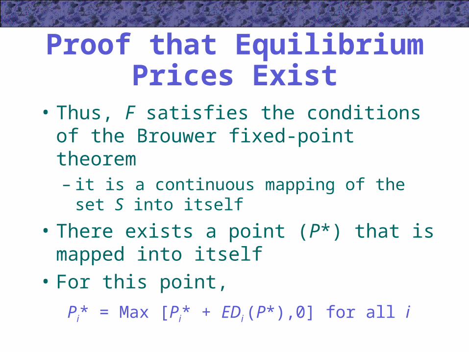
• Thus, F satisfies the conditions of the Brouwer fixed-point theorem– it is a continuous mapping of the set S into

itself

• There exists a point (P*) that is mapped into itself

• For this point,

Pi* = Max [Pi* + EDi (P*),0] for all i


• This says that P* is an equilibrium set of prices– For Pi* > 0,

Pi* = Pi* + EDi (P*)

EDi (P*) = 0– For Pi* = 0,

Pi* + EDi (P*) 0

EDi (P*) 0

A General Equilibrium with Three Goods

• The economy of Oz is composed only of three precious metals: (1) silver, (2) gold, and (3) platinum– there are 10 (thousand) ounces of each

metal available

• The demands for gold and platinum are

1121

3

1

22

P

P

P

PD 182

1

3

1

23

P

P

P

PD


• Equilibrium in the gold and platinum markets requires that demand equal supply in both markets simultaneously

101121

3

1

2 P

P

P

P

101821

3

1

2 P

P

P

P


• This system of simultaneous equations can be solved as

P2/P1 = 2

P3/P1 = 3

• In equilibrium:– gold will have a price twice that of silver– platinum will have a price three times that

of silver– the price of platinum will be 1.5 times that

of gold


• Because Walras’ law must hold, we knowP1ED1 = – P2ED2 – P3ED3

• Substituting the excess demand functions for gold and silver and substituting, we get

31

23

1

322

1

32

1

22

11 822 PP

P

P

PPP

P

PP

P

PEDP

1

3

1

22

1

23

21

22

1 822P

P

P

P

P

P

P

PED

Money in General Equilibrium Models

• Competitive market forces determine only relative and not absolute prices

• To examine how the absolute price level is determined, we must introduce money into our models


• Money serves two primary functions in any economy– it facilitates transactions by providing an

accepted medium of exchange– it acts as a store of value so that economic

actors can better allocate their spending decisions over time


• One of the most important functions played by money is to act as an accounting standard

• A competitive market system for n goods can generally arrive at an equilibrium set of prices (P1,…,Pn)

– these prices are unique only up to a common multiple

• only relative prices can be determined


• In principle, any good (k) could be chosen as the accounting standard– the prices of the other n-1 goods would be

referred to in terms of the price of k– the relative prices of the goods will be

unaffected by the choice of k

• Societies generally adopt fiat money as the accounting standard


• In an economy where money is produced in a way similar to any other good (commodity money), the relative price of money is determined by the forces of demand and supply– if gold is used, new discoveries will increase

the supply of gold, lower its relative price, and increase the relative prices of other goods


• With fiat money, the government is the sole supplier of money and can generally choose how much it wishes to produce

• Classical economists suggested that the economy can be dichotomized into two sectors– real: where relative prices are determined– monetary: where the absolute price level is

set


• Classical economists argued that the quantity of money available has no effect on the real sector

• This “classical dichotomy” only holds if:– individuals’ MRS between two real commodities

is independent of the amount of money available

– firms’ RPT between two real commodities is independent of the amount of money available


• The classical dichotomy will hold if firms and individuals only choose to hold money in order to perform transactions– money yields no utility or productivity

• If there are two nonmonetary goods (X and Y) in the economy, total transactions will be PX*X + PY*Y


• Conducting these transactions requires that a fraction () of their total value be available as circulating money

• The demand for money will be

DM = (PX*X + PY*Y)

• Monetary equilibrium requires that

DM = SM


• A doubling of the money supply would throw this system into disequilibrium– there would be an excess supply of

money– according to Walras’ law, this would be

balanced by a net excess demand for goods


• Equilibrium could be restored by a precise doubling of equilibrium nominal prices– the transactions demand for money would

double but relative prices would not change

Important Points to Note:

• Simple Marshallian models of supply and demand in several markets may not in themselves be adequate for addressing general equilibrium questions– they do not provide a direct way to tie

markets together and illustrating the feedback effects that occur when market equilibria change

Important Points to Note:

• A simple general equilibrium model of relative price determination for two goods can be developed using an indifference curve map to represent demands for the goods and the production possibility frontier to represent supply– this model is useful for examining

comparative statics in a general equilibrium context

Important Points to Note:• Construction of the production possibility

frontier from the Edgeworth box diagram permits an integration of factor markets into a simple general equilibrium model– the shape of the production possibility

frontier shows how reallocating factors of production among outputs affects the marginal costs associated with those outputs

– the slope of the production possibility frontier (RPT) measures the ratio of marginal costs

Important Points to Note:• Whether a set of competitive prices

exists that will equilibrate many markets simultaneously is a complex theoretical question– such a set of prices will exist if demand

and supply functions are suitably continuous and if Walras’ law (which requires that net excess demand be zero at any set of prices) holds

Important Points to Note:• Incorporating money into a general

equilibrium model is a major focus of macroeconomic research– in some cases, such monetary models will

exhibit the classical dichotomy in the monetary forces will have no effect on relative prices observed in the “real” economy

• these cases are rather restrictive so the extent to which the classical dichotomy holds in the real world remains an unresolved issue

chapter 16 general competitive equilibrium copyright ©2002 by south-western, a division of thomson...

Documents