chapter 2 describing motion: kinematics in one...
TRANSCRIPT
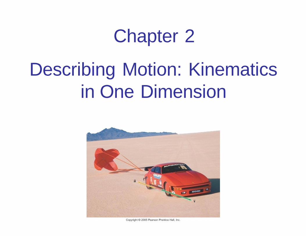
Chapter 2
Describing Motion: Kinematics in One Dimension

• Introduction
• Reference Frames and Displacement
• Average Velocity
• Instantaneous Velocity
• Acceleration
• Motion at Constant Acceleration
• Falling Objects
(previous lecture)
(previous lecture)
(previous lecture)
(previous lecture)
(previous lecture)

Recalling Last LectureRecalling Last Lecture
You need to defi ne a reference frame in order to ful ly characterize the motion of an object. In general, we use Earth as reference frame forour measurements.
Displacement is how far an object is found from its initial position after an interval of time Δt:
Eq. 2.1 gives the magni tude of the vector
Average velocity is given by:
And average acceleration is:
Both velocity and acceleration are vectors (give direction and magni tude) :
(2.1) x1 x2
(2.4)
(2.6)
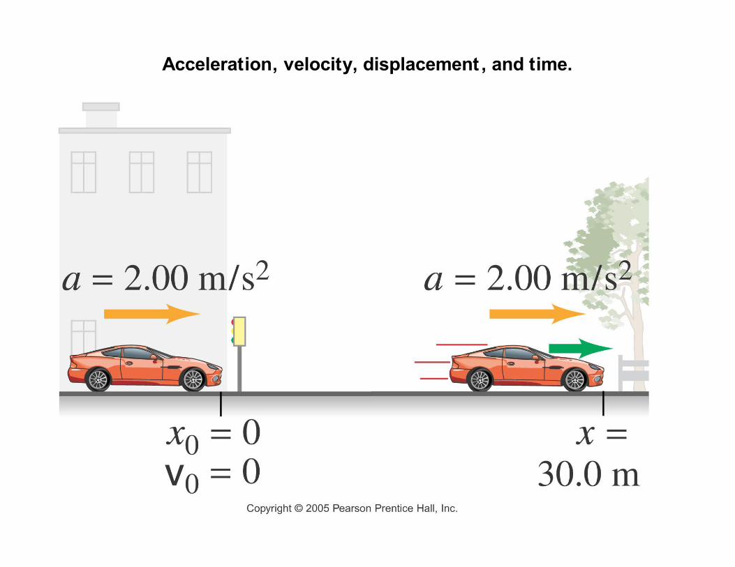
Acceleration, velocity, displacement , and time.
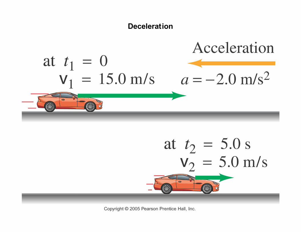
Deceleration

The car from the previous example, now moving to the left and decelerating.
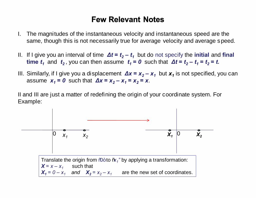
Few Relevant NotesFew Relevant Notes
I. The magnitudes of the instantaneous velocity and instantaneous speed are the same, though this is not necessarily true for average velocity and average s peed.
II. If I give you an interval of time Δt = t2 – t1 but do not specify the initial and final time t1 and t2 , you can then assume t1 = 0 such that Δt = t2 – t1 = t2 = t.
III. Similarly, if I give you a displacement Δx = x2 – x1 but x1 is not specified, you can assume x1 = 0 such that Δx = x2 – x1 = x2 = x.
II and III are just a matter of redefining the origin of your coordinate system. For Example:
0 0x2x1 X1 X2
Translate the origin from “0” to “x1” by applying a transformation:X = x – x1 such that X1 = 0 – x1 and X2 = x2 – x1 are the new set of coordinates.

Motion at Constant AccelerationMotion at Constant Acceleration
It is not unusual to have situations where the acceleration is constant. In this lecture, we will see one of such situations experienced by you in your everyday l ife. But before, let’s assume a motion in a straight line subject to a constant acceleration. In this case the following is valid:
à The instantaneous acceleration and the average acceleration have the same magnitude. We can then write:
We will use item II from the previous slide with following conventions:
t1 = 0 , t2 = t
and also define the position and velocity at t1 = t = 0 as
x1 = x0 , x = x2v1 = v0 , v = v2
for our future developments.
(2.8)

Motion at Constant AccelerationMotion at Constant Acceleration
With this in mind, let’s find some useful equations relating a, t, v, v0, x and x0 for cases with constant acceleration such that you can calculate any unknown variable if you know the others .
Let’s first obtain an equation to calculate the velocity v of an object subjected to a constant acceleration a:
Using the definitions introduced on the previous slide, we can rewrite eq. 2.6 as :
Eq. 2.10 can be rearranged:
Eq. 2.10 allows you to calculate the velocity v of an object at a given time t knowing its acceleration a and initial velocity v0.
(2.9)
(2.10)
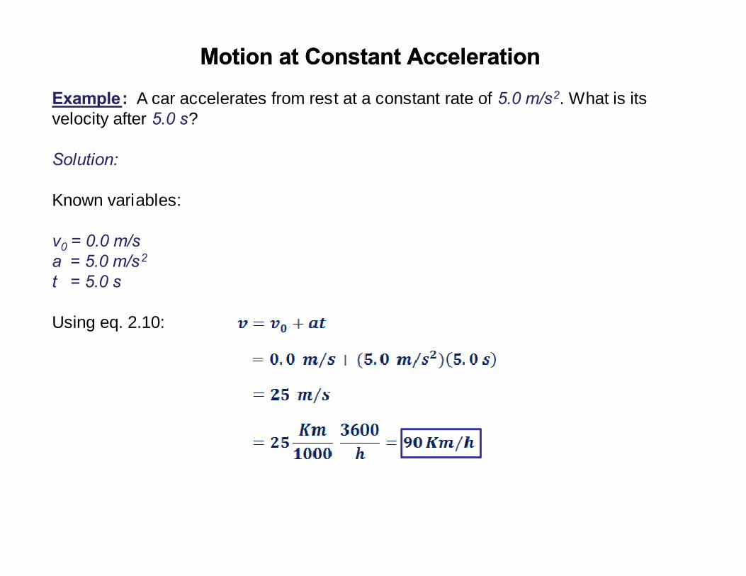
Motion at Constant AccelerationMotion at Constant Acceleration
Example: A car accelerates from rest at a constant rate of 5.0 m/s2. What is its velocity after 5.0 s?
Solution:
Known variables:
v0 = 0.0 m/sa = 5.0 m/s2
t = 5.0 s
Using eq. 2.10:
Motion at Constant AccelerationMotion at Constant Acceleration
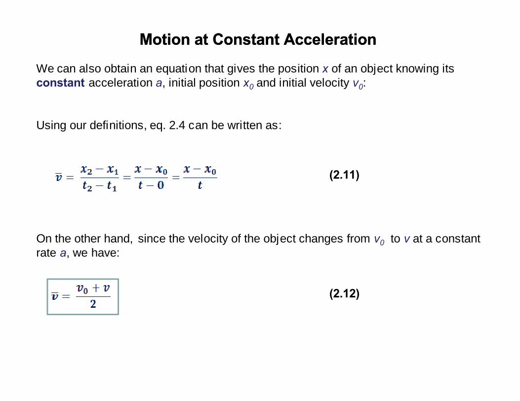
We can also obtain an equation that gives the position x of an object knowing its constant acceleration a, initial position x0 and initial velocity v0:
Using our definitions, eq. 2.4 can be written as:
On the other hand, since the velocity of the object changes from v0 to v at a constant rate a, we have:
(2.11)
(2.12)
Motion at Constant AccelerationMotion at Constant Acceleration
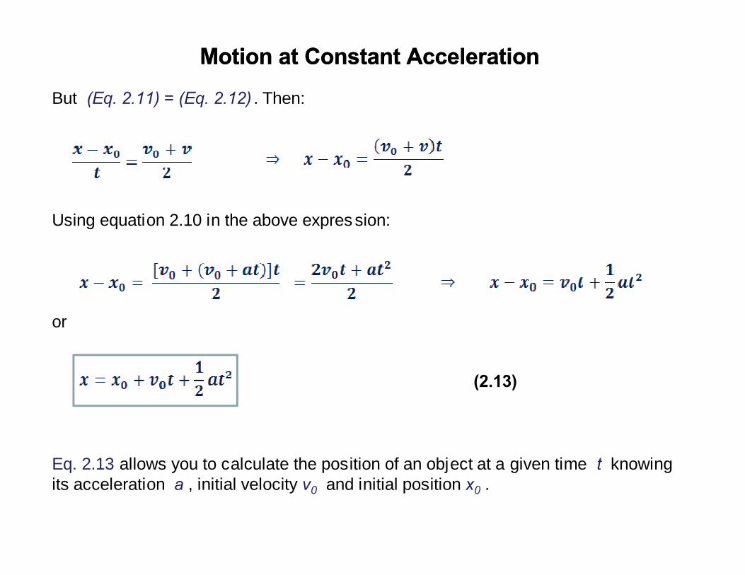
But (Eq. 2.11) = (Eq. 2.12) . Then:
Using equation 2.10 in the above expres sion:
or
Eq. 2.13 allows you to calculate the position of an object at a given time t knowing its acceleration a , initial velocity v0 and initial position x0 .
(2.13)
Motion at Constant AccelerationMotion at Constant Acceleration
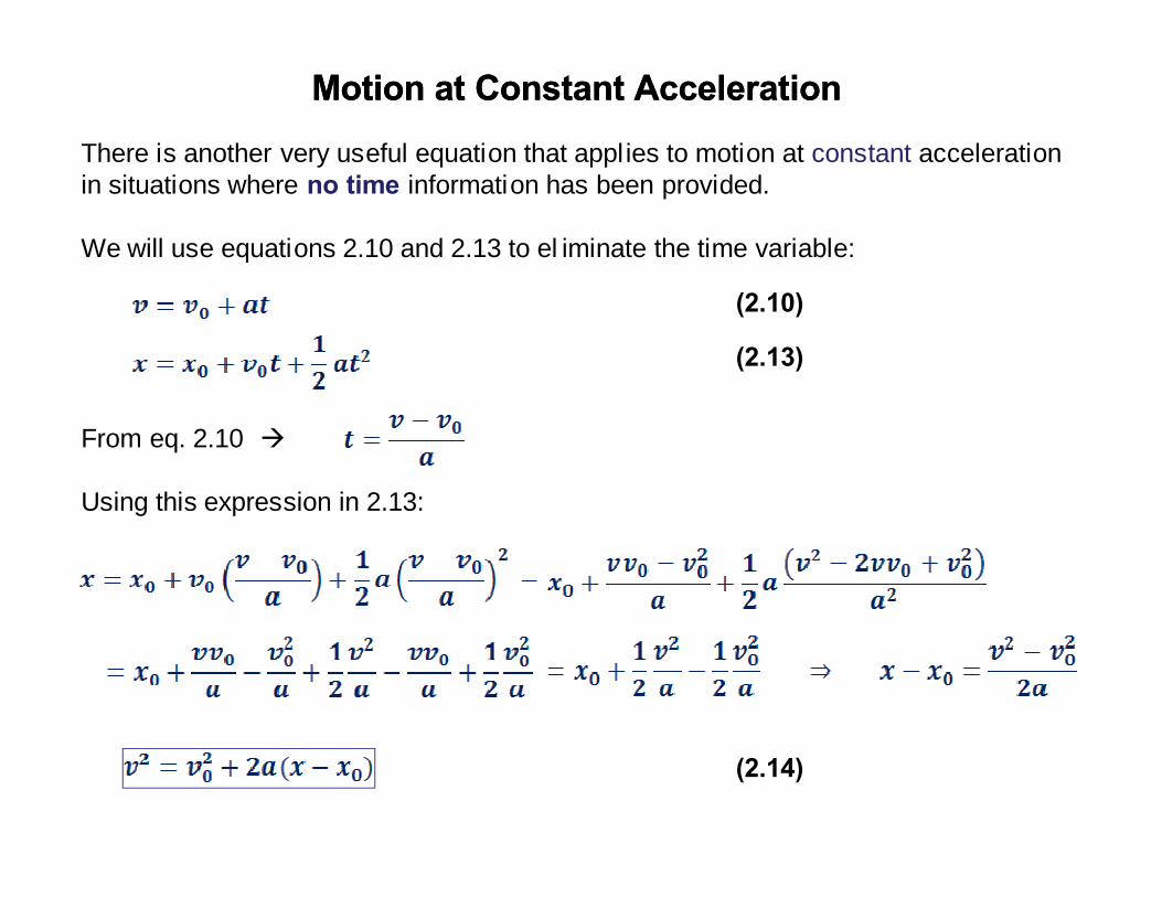
There is another very useful equation that appl ies to motion at constant acceleration in situations where no time information has been provided.
We will use equations 2.10 and 2.13 to el iminate the time variable:
From eq. 2.10 à
Using this expression in 2.13:
(2.10)
(2.13)
(2.14)

Motion at Constant AccelerationMotion at Constant Acceleration
Example (Problem 28 from the text book): Determine the stopping distances for a car with an initial speed of 95 Km/h and human reaction time of 1.0 s, for an acceleration (a) a = -4.0 m/s2 ; (b) a= -8.8 m/s2 ?
Solution:
We want to convert from h to s. It is also wise to convert from Km to m:
(remember to c arry some extra figures through your calculations)
Next, we have to define our reference frame (coordinate system)in order to calculate the positionwhere the driver starts breaking.
Driver realizes he has to brake (v = v0)
Driver starts braking (v = v0)
cars stops (v = 0)
0 xx0

Motion at Constant AccelerationMotion at Constant Acceleration
Continuing…………
Note that no information on the time needed to stop the car is provided. This problem is better approac hed with eq. 2.14. The position where the brak es are appl ied can be obtained if we observe that the car is moving at constant velocity v0 before the dri ver reacts. We can then use the equation of motion for constant velocity to find x0:
As we have already mentioned, the final velocity v is zero in both (a) and (b) c ases:
v (final) = 0.0 m/s
(continue on the next slide)
Motion at Constant AccelerationMotion at Constant Acceleration
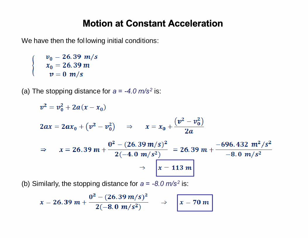
We have then the fol lowing initial conditions:
(a) The stopping distance for a = -4.0 m/s2 is:
(b) Similarly, the stopping distance for a = -8.0 m/s2 is:

Motion at Constant AccelerationMotion at Constant Acceleration
Let’s summarize the set equations we just found:
Note that these equations are only valid when the acceleration is constant.
(2.12)
(2.14)
(2.13)
(2.10)
Motion at Constant AccelerationMotion at Constant Acceleration
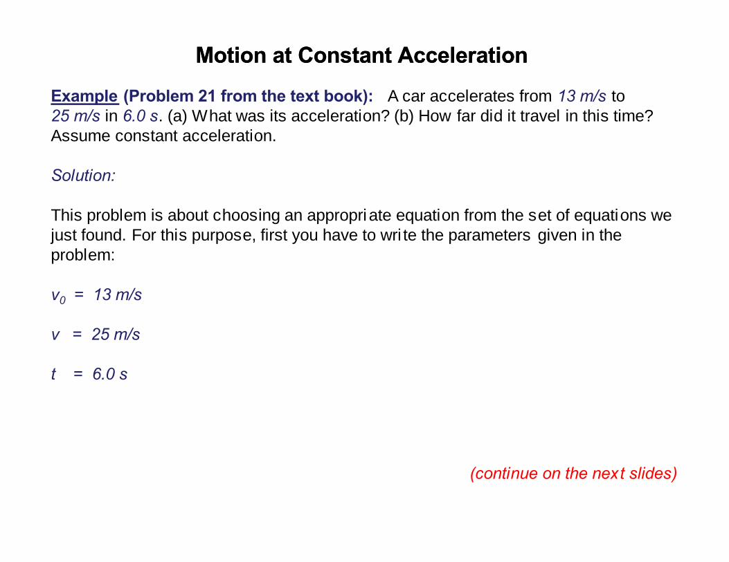
Example (Problem 21 from the text book): A car accelerates from 13 m/s to 25 m/s in 6.0 s. (a) What was its acceleration? (b) How far did it travel in this time? Assume constant acceleration.
Solution:
This problem is about choosing an appropriate equation from the set of equations we just found. For this purpose, first you have to wri te the parameters given in the problem:
v0 = 13 m/s
v = 25 m/s
t = 6.0 s
(continue on the next slides)

Motion at Constant AccelerationMotion at Constant Acceleration
(a) Here you want a knowing v0 , v and t. Which of the equati ons below you find more appropriate to solve this problem?
It is clear that 2.10 is the better choice for this item.
;
(2.12)
(2.14)
(2.13)
(2.10)
Motion at Constant AccelerationMotion at Constant Acceleration
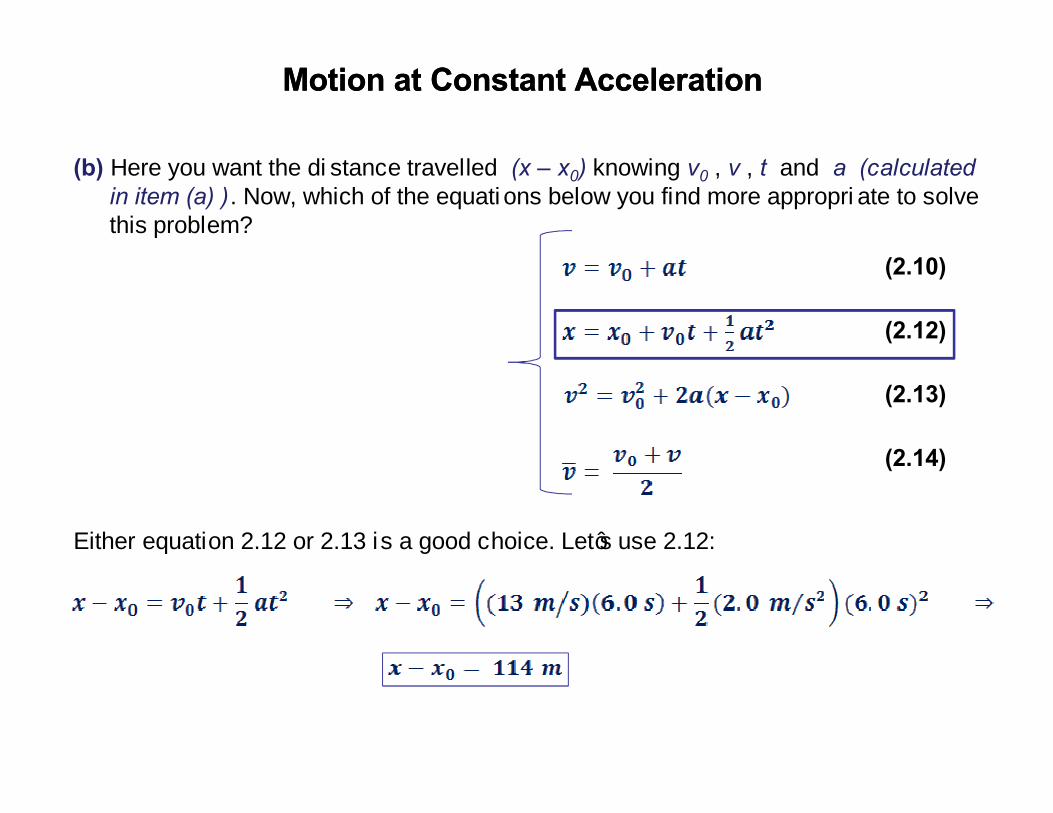
(b) Here you want the di stance travelled (x – x0) knowing v0 , v , t and a (calculated in item (a) ). Now, which of the equati ons below you find more appropri ate to solve this problem?
Either equation 2.12 or 2.13 is a good choice. Let’s use 2.12:
(2.12)
(2.14)
(2.13)
(2.10)

FallingFalling ObjectsObjects
We know from observation that an object will fall if we through it from a bridge. It will in fact gain speed as it falls. In other words , it is being accelerated.
This acceleration is due to the action of the Earth gravi tational force upon the object. We will come back to gravitation in few lectures from now.
We use the letter g to denote the gravitational acceleration.
à g is always different from zero at any pos ition but the very center of the Earth.
We can say to very good approximation that g is constant:
(2.15)
FallingFalling ObjectsObjects
Some Notes:
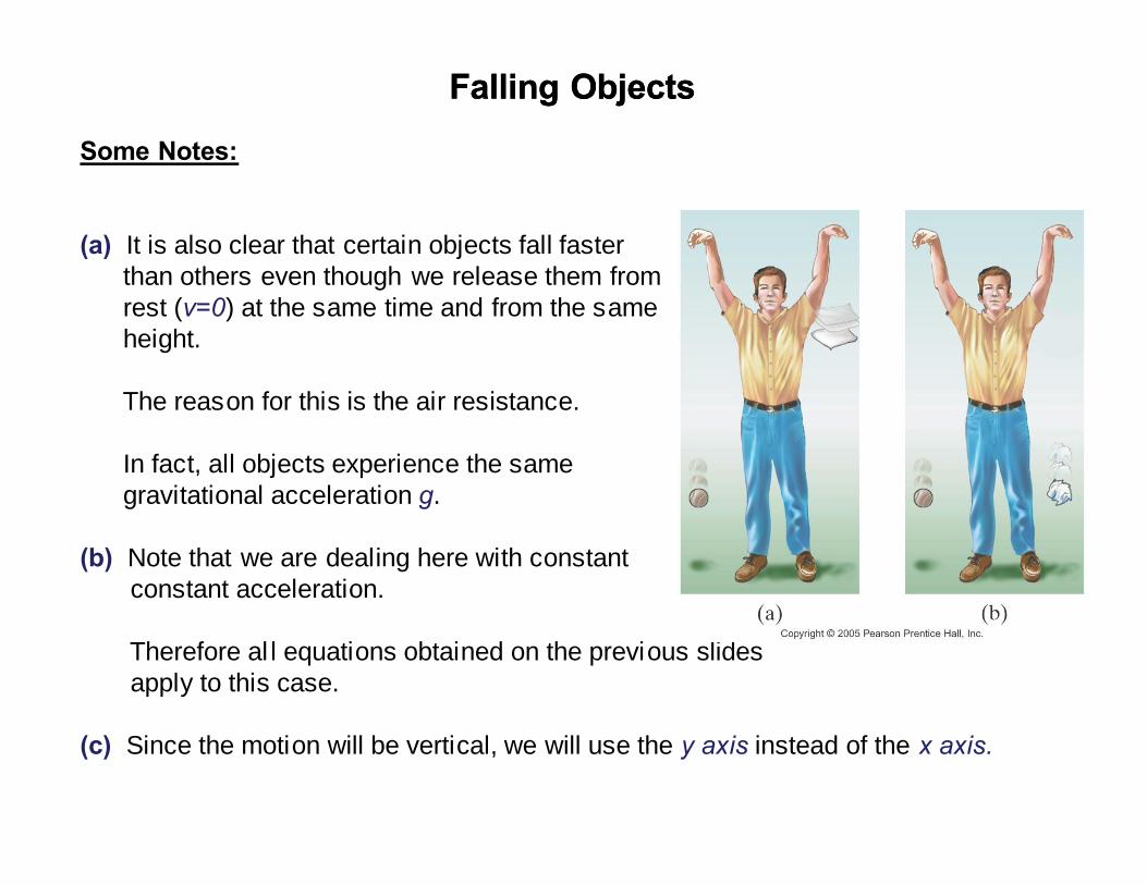
(a) It is also clear that certain objects fall faster than others even though we release them from rest (v=0) at the same time and from the same height.
The reason for this is the air resistance.
In fact, all objects experience the same gravitational acceleration g.
(b) Note that we are dealing here with constantconstant acceleration.
Therefore al l equations obtained on the previous slides apply to this case.
(c) Since the motion will be vertical, we will use the y axis instead of the x axis.

FallingFalling ObjectsObjects
Observing items (b) and (c) from the previous slide, we can rewrite the equati ons of motion as:
Note: In most cases we will ignore the ai r resistance, unless otherwise stated.
(2.17)
(2.19)
(2.18)
(2.16)

FallingFalling ObjectsObjects
Example (Problem 35 from the textbook): Estimate (a) how long it took King Kong to fall straight down from the top of the Empi re State Building (380 m high), and (b) his velocity just before “landing”?
Solution:
Let’s chose downwards as the positive y direction (again, this is just a convention).
Again, we have to identify the initial conditions.
g = 9.80 m/s2
y - y0 = 380 m
v0 = 0.0 m/s
(continue on the next slides)
380 m
+y

FallingFalling ObjectsObjects
(a) Here you want t knowing v0 , g and (y – y0) . Which of the equations below you find more appropriate to solve this problem?
Equation 2.17 is more appropri ated here:
Here, the minus sign is not physical since it would imply King Kong traveling back time à
(2.17)
(2.19)
(2.18)
(2.16)
FallingFalling ObjectsObjects
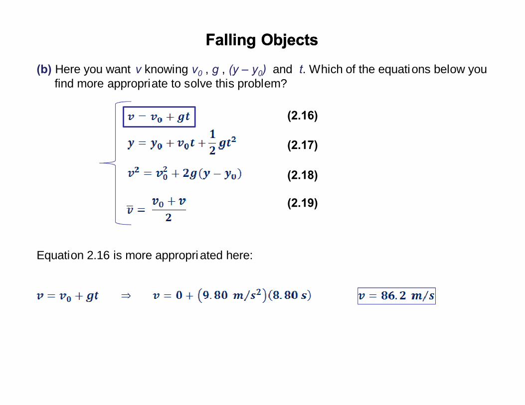
(b) Here you want v knowing v0 , g , (y – y0) and t. Which of the equations below you find more appropriate to solve this problem?
Equation 2.16 is more appropri ated here:
(2.17)
(2.19)
(2.18)
(2.16)