9

CHAPTER 2

LITERATURE REVIEW

2.1 INTRODUCTION

There are two main practical problems that engineers face in a

manufacturing process. The first is to determine the values of the process

parameters which yield the desired product quality (meet technical

specification) and the second is to maximize manufacturing system

performance using the available resources. The decisions made by

manufacturing engineers are based on conventions regarding the phenomena

that take place during processing. In the grinding process, many of these

phenomena are highly complex and interact with a large number of factors,

thus preventing high process performance form being attained. To overcome

these problems, the researchers propose models that try to simulate the

conditions during grinding and establish cause and effect relationships

between various factors and desired product characteristics.

Further more, the technological advances in the field, for instances

the ever growing use of computer controlled machine tools, have brought up

new issues to deal with, which further emphasize the need for more precise

predictive models. The developments of wear resistant abrasives, powerful

machinery and adequate machining technologies have lead to a considerably

increased efficiency of the grinding process. The economical advantages thus

achieved are consolidated and extend the position of grinding technology, the

grinding process being a quality defining finishing method. The grinding

10

process has been the object of technological research for some decades now.

This chapter is to present the various methodologies and strategies that are

adopted by researchers in grinding optimization and different techniques used

by the researchers in multi-objective optimization in grinding process.

2.2 GRINDING - OVERVIEW

Machining is the commonly used manufacturing process for the

production of finished components of desired shape, size and accuracy.

Machining process involves the usage of single or multiple point cutting tools

to remove the unwanted materials from the stock in the form of chips

(Komandurai 1993). Grinding is a manufacturing process with unsteady

process behaviour, whose complex characteristics determine the technological

output and quality.

2.2.1 Grinding principles

Grinding removes the metal from the work piece in the form of

small chips by mechanical action of abrasive particles bonded together in a

grinding wheel. Rubbing, Plowing and Metal removal are the three stages of

chip removal process in grinding (Rajmohan and Radhakrishnan 1990).

Grinding is a slow process in terms of unit removal of the stock. Hence, other

methods are used first to bring the work closer to its required dimensions and

then it is ground to achieve the desired finish. In some applications, grinding

is also employed for higher metal removal rate. In such heavy duty grinding

operations more abrasive is consumed. In these cases, the main objective is to

remove more amount of material that too as quickly and effectively as

possible. Thus, the grinding process can be applied successfully to almost

any component requiring precision or hard machining and it is also one of the

widely used methods of removing material from the work piece after

hardening.

11

The process quality depends on a large extent on the experience of

the operator. Within the spectrum of machining processes, the uniqueness of

grinding is found in its cutting tool. Modern grinding wheels and tools are

generally composed of two materials, one is the tiny abrasive particles called

grains or grits which do the cutting and the other is a softer bonding agent to

hold the countless abrasive grains together in a solid mass (Figure 2.1).

Figure 2.1 Grinding wheel showing edge of abrasive grains projecting

from the face

Grinding is an abrasive manufacturing process with a large number

of interacting variables, which depends on the type of grinding employed.

Grinding is very complex process since more interactions are involved in the

grinding zone (Figure 2.2) and difficult to study because of the small size of

the individual chips produced by hard abrasive particles having wide range of

shape, spacing and random geometry (Akira and Tadaaki 1966, Subramanian

and Ramnath 1992 ).

12

Figure 2.2 Microscopic interactions in the grinding zone

Since grinding wheels can be classified as composite materials, the

structural arrangement of the abrasive grain and binder can greatly affect their

elastic properties. Brecker (1974) analyzed bond formation during firing of

vitrified wheels and observed the cross section of the wheel, from which he

concluded that surface tension forces are sufficient to draw the abrasive grains

into direct contact.

When high accuracy of the work-piece and the automation of the

grinding work are considered, it is necessary to secure the reliability and the

reproducibility for grinding wheel as a cutting tool. For this purpose, it is

important to choose a grinding wheel of uniform grade. However, irregularity

of grade changes the grinding characteristic on the working periphery of a

grinding wheel locally and it affects the dimensional accuracy of work-piece

(Shinichi Tooe et al 1987).

13

During grinding, material is removed from the work-piece surface in

the form of small chips by the abrasive particles on the grinding wheel. The

material removal can be visualized by considering a single abrasive grain on

the wheel (Figure 2.3). As the grain makes contact with the work-piece

surface, the depth of cut is zero.

Figure 2.3 Grinding principles

As the wheel and work-piece revolve, the depth of cut increases to a

maximum, some where along the arc of contact of the wheel and the work-

piece and then reduces again when the chip is dislodged from the work-piece.

Since the wheel speed is considerably higher than the work speed, the

maximum value of depth of cut is reached almost at the point where the wheel

leaves the work-piece. This depth of cut is termed as the grain depth of cut.

In Figure 2.3, when the grain is at P it is just contacting the work-

piece and the depth of cut is zero. In unit time T, the grain will advance to

position R. In the same unit time T, the point R on the work-piece would

have come to position S. The point S will be very near to the point R, since

14

the rotation of the wheel is much faster than the work. The chip section

removed is represented by PRS. The maximum depth of cut represented by

SU is the maximum chip thickness per grit (or) the grain depth of cut (gd).

The length traversed by the abrasive grain PR in unit time

T = PR = Vs T or T = PR/ Vs (2.1)

where Vs = Surface speed of the wheel in m/s.

The length traversed by the point R on the work-piece in unit time

T = RS = Vw T (2.2)

where Vw =Surface speed of the work in m/s

Maximum chip thickness per grit

SU = RS sin ( ) (2.3)

where and are the angles subtended at the centers of the grinding wheel

and the work-piece by the point R.

Therefore,

SU = Vw T sin ( ) (2.4)

If there are Z numbers of grains in unit length, the number of grains in length

PR of the grinding wheel is given by PR *Z

Maximum chip thickness per grit, gd =SU

PR.Z (2.5)

15

gd = wV TSU [sin( )]PR.Z PR.Z

(2.6)

Substituting for T

gd = w

s

V sin( )ZV

(2.7)

The wheel can be made to cut harder or softer by reducing or

increasing the grain depth of cut. It can be seen from the equation (2.7) the

following are clear.

i) Work speed – By increasing the work speed, the grain depth

of cut increases and the bond wears out faster and the wheel

appears softer. When the work speed decreases, the wheel

appears to be harder.

ii) Wheel speed – By reducing the wheel speed the grain depth

increases and the wheel appears softer. By increasing the

wheel speed, the wheel appears harder (Arabatti et al 1996).

2.2.2 Grinding Parameters

The success of any grinding operation depends on the proper

selection of various grinding parameters, like wheel speed, work speed,

transverse feed, and in-feed area of contact, grinding fluids, balancing of

grinding wheels and dressing etc. Subramanian and Lindsay (1992) have

given the concept of grinding system approach that addresses four key inputs

to the grinding process viz. machine tool, wheel selection, work material

properties and operational factors (Figures 2.4 and 2.5). Inadequate attentions

to details in any one of these systems input parameters can result in uncertain

grinding results.

16

Figure 2.4 Input/Output model of the precision grinding process

Input

Process

Output

Machine toolSuper abrasive wheelWork materialOperational factors

Grinding Forcesand Energy

Surface generationWheel wearChipsCoolant interactions

o Cuttingo Plowingo Rubbing

Part qualityProduction economicsNew products/ processesSurface integrityResidual stress

17

Figure 2.5 Variables influencing the grinding process

Machine tool factorsDesign

Rigidity Precision Dynamic stability

Features Controls Power, speed etc., Slide movements Truing and dressing

Coolant Type, pressure, flow Filtration systems

Improved grinding resultso Surface quality Retained strengtho Tolerances / Finish Production rateo Cost per part Product

performance

Operational factors

Fixtures

Wheel balancing

Truing, dressing andconditioning techniques,devices, parameters

Grinding cycle design

Coolant application

Inspection methods

Wheel selection factorsAbrasive

Type Properties Particle size Distribution Concentration

Bond Type Hardness /grade Stiffness Porosity Thermal conduction

Wheel design Shape/size Core material

Work material factorsProperties

Mechanical Thermal Chemical Abrasion resistance Microstructure

Geometry Wheel-part conformity Shape required

Part quality Geometry Tolerances Consistency

18

2.2.3 Influence of input process parameters

A very large number of widely varying parameters affects the

grinding process. Unlike most of the input values like the machine, grinding

wheel, machine setting, etc., which can be optimized, the work material which

is selected in view of the required properties of the finished product, cannot

be changed. Therefore, in order to achieve a well-adjusted grinding process,

the variable process input values must be adapted to the material. The

grinding process is characterized by grinding power, forces, vibration,

temperature, wheel wear and wheel loading (Figure 2.6).

Figure 2.6 Influences of process input on grinding process and work

quality

InteractionGrinding powerGrinding forceMechanical wearHeat generationWheel loading

Workpiece quality Accuracy in sizeAccuracy in shapeLess thermal effectsResidual stressesChange in hardness

Process inputMachineGrinding wheelWork materialMachine settingsAuxiliary

Grinding process

19

2.2.4 Wheel wear

The geometry of grits on the wheel surface continuously alters due

to the influence of cutting mechanisms and forces. The condition of the

wheel is also altered due to the wear of the grinding wheel and by the loading

of the work material into its pores. Wheel wear and loading bring down the

cutting efficiency and the grinding forces increase gradually (Chander et al

1978).

Wear of grinding wheel may be defined as the loss of abrasives

from the surface of the wheel and are due to (i) attritious wear of grains

(ii) mechanical grain fracture and (iii) rupture of bond or gross pullout of

whole grain (Pande and Lal 1976). Attritious wear is a gradual dulling or

flattering of abrasive grains by rubbing against the work-piece. This type of

wear has much influence on the cutting action of abrasive grain and the

cutting forces are dependent on it. Such a wear occurs mostly under mild

grinding conditions in precision grinding. It generates wear flats on the grain

thus reducing the cutting efficiency of the grains. Severe grinding conditions

subject the wheel material to fracture and the surface is modified constantly

due to self-sharpening phenomenon. Grain fracture occurs as a result of

mechanical forces associated with chip formation or due to thermal shock

induced by instantaneous high temperatures. Gross pullout or bond fracture

depends upon the tensile stresses in the bond bridge, which in turn depends on

the grade of the wheel (Yoshikawa and Sata 1963).

Wheel wear rate is found to be an exponential function of grinding

force. As the grinding process is continued, the wheel loses its form due to

non-uniform removal of material on the wheel surface. Hence, the condition

of the wheel is continuously altered and a stage reaches after which the

20

grinding performance and efficiency starts deteriorating and starts adversely

affecting the work-piece finish and surface integrity.

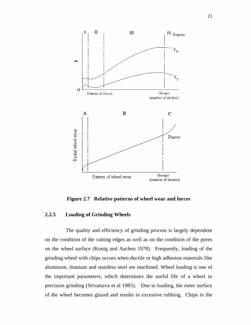
The pattern of wheel wear and its associated pattern of forces are

shown in Figure 2.7. The wheel wear pattern may be classified into three

phases.

i) Phase A – intensive wheel wear and it is related to the wheel

dressing techniques,

ii) Phase B – a constant time – rate of wear under good grinding

conditions remains constant over long period. This is the

optimum condition for economic grinding practice and

iii) Phase C – results when either the wheel is overloaded or

excessive vibrations occur and wheel wear occurs due to

bond post rupture. Whole grits are being dislodged from the

wheel.

Wheel wear measured from the reduction in wheel diameter does not

give accurate estimate of the wheel wear. From the wear particle size

distribution analysis of the wheel, wear can be ascertained accurately but the

procedure is cumbersome (Grisbrook et al 1962). The rate of wheel wear

depends upon the work speed, wheel speed and grinding depth. Employing

reduced wheel speeds can reduce wheel wear. Low work speeds will reduce

the wheel wear for the same metal removal rate but it may cause thermal

damage to the work-piece (Malkin and Cook 1971).

21

Figure 2.7 Relative patterns of wheel wear and forces

2.2.5 Loading of Grinding Wheels

The quality and efficiency of grinding process is largely dependent

on the condition of the cutting edges as well as on the condition of the pores

on the wheel surface (Konig and Aachen 1978). Frequently, loading of the

grinding wheel with chips occurs when ductile or high adhesion materials like

aluminum, titanium and stainless steel are machined. Wheel loading is one of

the important parameters, which determines the useful life of a wheel in

precision grinding (Srivatsava et al 1985). Due to loading, the outer surface

of the wheel becomes glazed and results in excessive rubbing. Chips in the

22

grinding wheel will alter the grain edge geometry and the friction process

occurring during grinding operations. The loaded wheel will result in

increased cutting forces and grinding power consumption, which in turn may

lead to a breakdown of the grinding wheel structure.

The loaded wheel also generates more heat, which in turn affects the

surface integrity of the work-piece such as surface roughness or surface

topography and surface metallurgy. Alterations of the surface layers include

plastic deformation, micro cracking, phase transformation, micro-hardness

changes, tears associated with built up edge and residual stress distribution

(Shah and Chawala 1979). To ensure consistent results in grinding, one has

to continuously investigate the condition or the modifications occurring on the

wheel and control them suitably.

If the cutting efficiency of the process is to be improved, the wheel

has to be provided with new sharp grains with porosity for chip flow. The

wheel is dressed to remove the clogged chips on the wheel material so that

new grains with sharp edges appear. One has to monitor continuously the

wheel condition and control them suitably to achieve consistent performance

in grinding.

2.2.6 Cylindrical Grinding

Cylindrical grinding designates a general category of various

grinding methods, which have the common characteristic of rotating the

work- piece about a fixed axis and grinding outside surface section in

controlled relation to that axis of rotation. In plunge type grinding machines

the wheel is plunged into the work at a predetermined feedrate and is

withdrawn at the time the workpiece reaches the correct size.

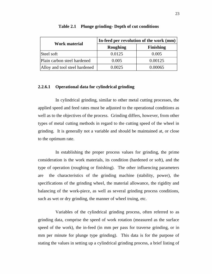
Table 2.1 gives general guideline about the depth of cut conditions followed

in plunge grinding.

23

Table 2.1 Plunge grinding- Depth of cut conditions

In-feed per revolution of the work (mm)Work material

Roughing FinishingSteel soft 0.0125 0.005Plain carbon steel hardened 0.005 0.00125Alloy and tool steel hardened 0.0025 0.00065

2.2.6.1 Operational data for cylindrical grinding

In cylindrical grinding, similar to other metal cutting processes, the

applied speed and feed rates must be adjusted to the operational conditions as

well as to the objectives of the process. Grinding differs, however, from other

types of metal cutting methods in regard to the cutting speed of the wheel in

grinding. It is generally not a variable and should be maintained at, or close

to the optimum rate.

In establishing the proper process values for grinding, the prime

consideration is the work materials, its condition (hardened or soft), and the

type of operation (roughing or finishing). The other influencing parameters

are the characteristics of the grinding machine (stability, power), the

specifications of the grinding wheel, the material allowance, the rigidity and

balancing of the work-piece, as well as several grinding process conditions,

such as wet or dry grinding, the manner of wheel truing, etc.

Variables of the cylindrical grinding process, often referred to as

grinding data, comprise the speed of work rotation (measured as the surface

speed of the work), the in-feed (in mm per pass for traverse grinding, or in

mm per minute for plunge type grinding). This data is for the purpose of

stating the values in setting up a cylindrical grinding process, a brief listing of

24

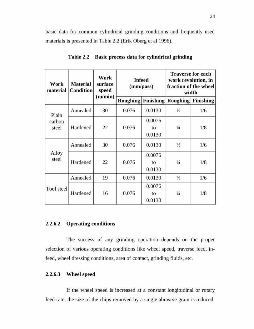
basic data for common cylindrical grinding conditions and frequently used

materials is presented in Table 2.2 (Erik Oberg et al 1996).

Table 2.2 Basic process data for cylindrical grinding

Infeed(mm/pass)

Traverse for eachwork revolution, in

fraction of the wheelwidth

Workmaterial

MaterialCondition

Worksurfacespeed

(m/min)Roughing Finishing Roughing Finishing

Annealed 30 0.076 0.0130 ½ 1/6Plain

carbonsteel Hardened 22 0.076

0.0076to

0.0130¼ 1/8

Annealed 30 0.076 0.0130 ½ 1/6Alloysteel Hardened 22 0.076

0.0076to

0.0130¼ 1/8

Annealed 19 0.076 0.0130 ½ 1/6

Tool steelHardened 16 0.076

0.0076to

0.0130¼ 1/8

2.2.6.2 Operating conditions

The success of any grinding operation depends on the proper

selection of various operating conditions like wheel speed, traverse feed, in-

feed, wheel dressing conditions, area of contact, grinding fluids, etc.

2.2.6.3 Wheel speed

If the wheel speed is increased at a constant longitudinal or rotary

feed rate, the size of the chips removed by a single abrasive grain is reduced.

25

This reduces the wear of the wheel. If the wheel speed is reduced, the wear is

increased. From this, it is clear that from the point of view of wear, it is better

to operate at higher wheel speeds (Opitz and Guhring 1968). However, this is

limited by the allowable speeds at which the wheel can be worked, as well as

the power and rigidity of the grinding machine. Normally, the grinding wheel

speed ranges from 20 to 40 m/sec. The wheel speed also depends upon the

type of grinding operation and the bonding medium of the grinding wheel

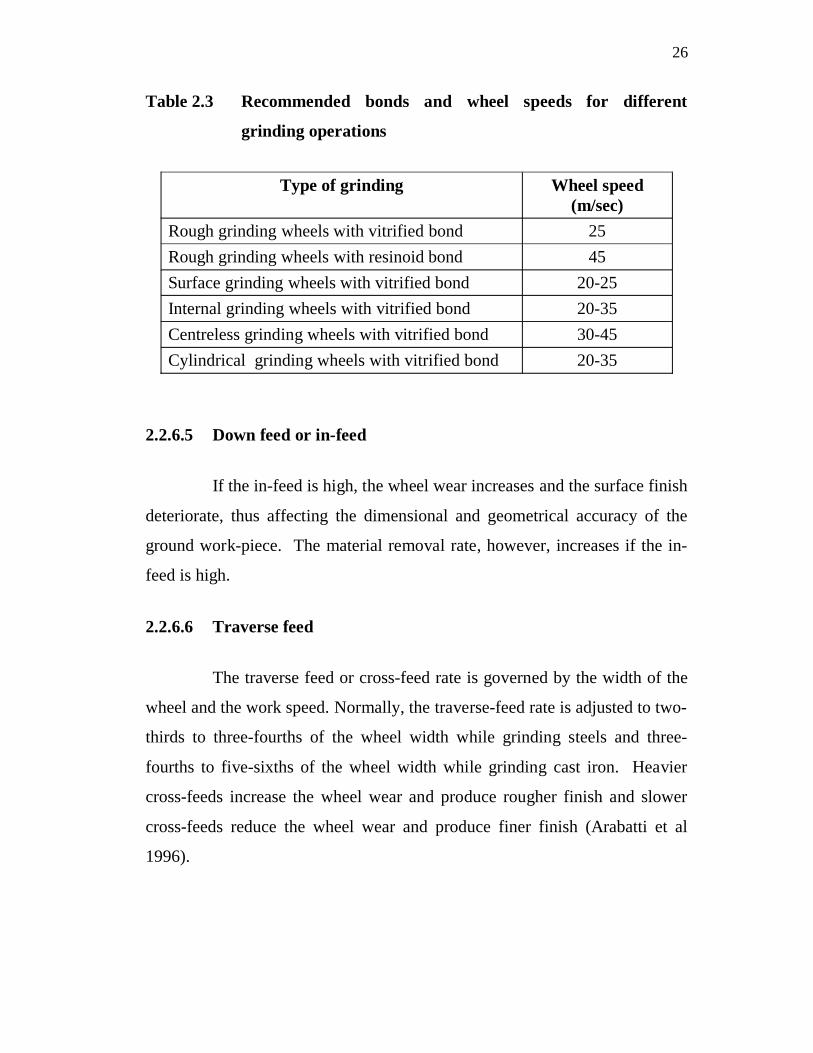
(Table 2.3). For example, resinoid bonded wheels can be generally used at

higher peripheral speeds than vitrified bond wheels.

2.2.6.4 Work speed

Work speed is the speed at which the work-piece traverses across

the wheel face or rotates between centers. If the work speed is high, the

wheel wear is increased but the heat produced is reduced. Hahn et al (1956)

stated that high work speeds are effective in reducing heat checks and

cracking of heat sensitive materials and may also influence the life of the tool

or part. On the other hand, if the work speed is low, the wheel wear decreases

but the heat produced is more. The ratio of wheel speed to work speed is of

much importance and it should be maintained at the proper value. Low work

speeds result in local overheating and bring about deformation or tempering

of the hardened work-piece. This in turn affects the mechanical properties of

the work piece and very often micro-cracks will appear on the work-piece.

The increase in work speed is limited by premature wheel wear and vibrations

induced by wear. Generally, if the wheel wear increases, the work speed

should be reduced. If the heat produced is high and clogging occurs,

especially with hard wheels, the work speed should be increased.

26

Table 2.3 Recommended bonds and wheel speeds for different

grinding operations

Type of grinding Wheel speed(m/sec)

Rough grinding wheels with vitrified bond 25Rough grinding wheels with resinoid bond 45Surface grinding wheels with vitrified bond 20-25Internal grinding wheels with vitrified bond 20-35Centreless grinding wheels with vitrified bond 30-45Cylindrical grinding wheels with vitrified bond 20-35

2.2.6.5 Down feed or in-feed

If the in-feed is high, the wheel wear increases and the surface finish

deteriorate, thus affecting the dimensional and geometrical accuracy of the

ground work-piece. The material removal rate, however, increases if the in-

feed is high.

2.2.6.6 Traverse feed

The traverse feed or cross-feed rate is governed by the width of the

wheel and the work speed. Normally, the traverse-feed rate is adjusted to two-

thirds to three-fourths of the wheel width while grinding steels and three-

fourths to five-sixths of the wheel width while grinding cast iron. Heavier

cross-feeds increase the wheel wear and produce rougher finish and slower

cross-feeds reduce the wheel wear and produce finer finish (Arabatti et al

1996).

27

2.2.6.7 Grinding Wheels

Grinding wheels are composed of selectively sized abrasive grains

held together by a bonding agent. The following influences the properties of

the grinding wheel (Jain and Gupta 2001):

i) Type of abrasives

ii) Grain size

iii) Type of bond

iv) Grade of the wheel

v) Structure of the wheel

Types of Abrasives: Grinding wheels are made of abrasive particles

bonded together by means of some suitable bonds. An abrasive is a harder

material which can be used to cut or wear away other materials. It is

extremely hard and tough, and when fractured, it forms sharp cutting edges

and corners. Abrasives particles used for grinding wheels of two types viz.,

(a) natural abrasives and (b) artificial abrasives. Generally for most of the

purposes, natural abrasives are not used due to certain advantages of artificial

abrasives. Most commonly used artificial abrasives are Silicon Carbide (SiC),

Aluminium oxide (Al2O3), Boron carbide and Boron Nitrate (CBN).

Grain Size: Grain size influences the stock removal rate and the

surface finish. Thw choice of grin size is determined by the nature of grinding

operation, material to be ground, material removal rate and surface finish

required. Coarser grits are used for heavy material removal rate and finer grits

for less material removal.

Type of Bond: A bond is a material that holds the abrasives grains

together enabling the mixture to be kept in a desired shape in the form of

28

wheel. The bonds most commonly used manufacturing of grinding wheels are

Vitrified bond (denoted by V), Silicate bond (S), Shallac bond (E), Rubber

bond (R) and Bakelite or resinoid bond (B). To obtain the maximum out of

the abrasive, it is important that the bond system is strong, versatile and has

superior corner holding properties. The idle bond system should facilitate a

uniform grain release, resulting in the wheel remaining free cutting for a

longer period of time. Extremely load resistant and free cutting bond system

will increase form holding capability result in reduction of dressing

frequency. This results in significant increase in wheel life. This also

improves the parts produced per hour due to savings in dressing time and

increased wheel life.

Grade of the Wheel: The grade of a wheel indicates the strength of

the grains and the holding power of the bond. It is usually referred to as

hardness of the wheel. A hard wheel wears down slowly and soft wheel wears

down readily. Hard wheel is used for precision grinding and for softer

material. The hardness of grinding wheel is classified as very soft (A to G),

soft (H to K), medium (L to O), hard (P to S) and very hard (T to Z).

Structure of the Wheel: Structure of a wheel refers to the voids

between abrasive particles. For a given bonding material thickness of void

size is controlled by the spacing of the grains and this structure may be dense

or open. Open structure wheel are used for high stock removal and dense

structured wheel for holding precision forms and profiles. The structure is

represented is by numbers ranging from 0 to 15, the lower numbers indicating

a dense structure and higher numbers represent open structure.

2.2.6.8 Wheel dressing

Wheel dressing is defined as the act of improving the cutting action.

It can also be described as sharpening operation. It becomes necessary from

29

time to time during the course of working to correct uneven wear and to open

up the face of the wheel so as to obtain efficient cutting conditions. Dressing a

wheel doest not necessarily true it. The wheel may be out of round or parallel

even after dressing as it only removes the outside layer of dulled abrasive

grains and the foreign material. Wheel dressing can be carried out with

diamond tool, which has a shearing action on the abrasive grains and the

bond, and so removes the dulled or irregular groups of grains. The diamond is

held in a holder. This is done by peening, brazing or securing the diamond by

casting a low melting point metal round it leaves sufficient of the stone

protruding for it to act as a cutting edge.

2.2.6.9 Area of grinding contact

The area of grinding contact between the wheel and the work affects

the choice of grit size and grade. The area of contact is relatively large in the

case of internal grinding and surface grinding and also when large diameter of

works are ground with a small diameter wheel. A larger area of contact

produces a lower pressure. On larger areas of contact and lower pressure, a

soft grade wheel provides normal breakdown of the grit, ensuring continuous

free cutting action. In addition, coarser grit is preferred to provide adequate

chip clearance between the abrasive grains. When the area of contact

becomes smaller, the pressure, which tends to break down the wheel face,

becomes greater, finer grit, and harder grade wheels should be used.

2.3 SUMMARY OF THE LITERATURE SURVEY

Many investigations have been done so far to specify the

relationship between grinding conditions and their influences on the

machining result. Optimization of machining processes is usually based on

finding operating conditions, which minimize machining costs or maximize

production rate. In order to perform such optimization analyses, a reliable

30

relationship between tool life and machining parameters (e.g., Taylor

equation) is generally required. Such optimization analyses can also be

applied to precision grinding process. Snoeys et al (1974) have proposed an

empirical tool life equation for plunge grinding assuming a power function

relationship between the volume removed per wheel dressing and the

equivalent chip thickness (removal rate per unit width divided by wheel

speed).

A major drawback with this relationship is the need for separate

evaluation of the constants in the tool life equation for each wheel -

workpiece combination, dressing procedure, wheel and work piece diameter

and even wheel speed. Other tool life relationships developed by Malkin

(1976) are based upon wear models of the grinding wheel up to burning, but

these are too complex for practical use. By making a quantitative energy

balance, Malkin (1975) showed that the total energy in grinding could be

considered as the sum of chip formation, plowing and sliding energies.

Plowing refers to work-piece deformation without removal and sliding energy

is associated with rubbing between the wear flats and the work-piece surface.

Both the plowing and sliding energy contributions become smaller at faster

removal rates, so that the minimum specific energy approaches the specific

energy for chip formation.

Mayne and Malkin (1976) have proposed an optimization approach

for plunge grinding of steels, in order to maximize the metal removal rate

subject to constraints on work piece burn and finish. In this approach, non-

linear optimization techniques have been applied to a generalized grinding

model and it was analytically demonstrated how the wheel dullness, as

indicated by wear flat area, influences the allowable removal rate. Selection

of optimal grinding conditions using this analysis is not practical because of

the need for having a reliable estimate of wear flat areas. Malkin and Yorem

31

Koren (1980), have developed a computer program for practical off-line

optimization of plunge grinding operation on steels based on the same

strategy is described above with additional relationship taking the dressing

parameter into account.

The modelling of grinding process requires the consideration of the

grinding wheel topography. Understanding the combined action of the cutting

edges, which are stochastically distributed on the grinding wheel, and the chip

formation process explains influences both on the grinding forces and the

surface roughness of the workpiece. According to Verkerk (1977), it is

sufficient to consider the cutting edges that belong to same grain as one

cutting edge. When there are more cutting edges on one grain, there is no

space for the chip between the cutting edges. Consequently, the cutting edges

can no longer be active. As a result, the grain acts as one cutting edge.

Verkerk gives a survey of the most important methods of measuring number

of static and kinematic grains. However, neither the measured grain count nor

the measured shape of the cutting edge tips can be used to draw direct

conclusion on the characteristics of the grinding wheel topography. The

topography models developed by the various researchers have the common

feature that many measurements are required to determine the model

parameters. Furthermore, the statistical geometrical distribution of the grains

is not taken into consideration. All these conclude that the practical

application of the topography models presented so far can be expected to be

time consuming, due to the measuring efforts necessary.

Surface integrity models describe the influences of mechanical and

thermal effects from grinding on the material of the work piece underneath

the work surface. The plastic deformations and the thermal influences on the

microstructure which occur during grinding can be revealed by changed

degrees of hardness on the underneath the work surface as well as by

32

metallographic examinations. In the most unfavourable case, grinding may

even lead to cracks, which have particularly negative effects on the

characteristics of the work piece. The generation of textures leads to

directional surface integrity characteristics. According to Tonshoff et al

(1992), many researchers have developed the surface integrity models,

however, the practical application of these models require much experimental

and measurement efforts.

Apart from modelling the surface integrity, the surface roughness is

a characteristic quantity, which determines the quality of the work piece and

thus it is of major importance. All the models developed so far have much

measuring effort that is necessary to determine the microstructure of the

grinding wheel. As a result, the practical application in today’s industry

requires an excessive number of efforts. Brown (1969) and Peters (1974) have

proposed a model to predict the surface roughness in grinding using

equivalent chip thickness. As this model does not describe the microstructure

of the grinding wheel, it can be used in industrial applications and assuming

stationary grinding process. Analytical models developed by the various

researchers for predicting surface roughness were based on the microstructure

of the grinding wheel in both one and two dimensions. The wheel

microstructure was described using simplification factors such as constant

distance between cutting edges and uniform height of the cutting edges.

Similar assumptions were used to describe the surface roughness based on

chip thickness models developed by Lal and Shaw (1975).

Empirical surface roughness models are a function of kinematic

condition, such as the one presented by Malkin (1989), and have had more

success in the industry because they do not need the effort of material and

surface wheel characterizations. However, the empirical constants involved

must be adjusted for every work piece material, lubricant, and type of wheel.

33

These models can be considered a subclass of empirical models due to the

empirical constants that need to be adjusted. None of the above mentioned

models was based on the stochastic nature of the grinding process, governed

mainly by the random geometry and random distribution of the cutting edges

on the wheel surface. To account for this, Inasaki (1996) has developed a

model to generate ground surface by simulation of the interaction of each

grain with the work piece material, where the relative cutting edge positions

were either randomly generated or deterministically given by measurement of

the wheel topography. Basuray et al (1980) made probably the only attempt to

develop a simple mathematical expression for the surface based on the

probabilistic analysis of their simulations; however, many parameters and the

material properties were lumped into empirical constraints.

Malkin (1978) determines the critical specific energy, which causes

work piece burn. The grinding energy model by Rowe (1988) is comparable

with Malkin’s model, but Rowe additionally takes the flow of heat into the

chips and the coolant into account. On this basis, he evaluates critical upper

and lower specific energy levels for thermal damage. The model for the

evaluation of the specific grinding energy by Inasaki et al (1989) has been

developed for the grinding of ceramics. The grinding energy is evaluated on

the basis of the theoretical cutting edge spacing. In this model, not the

generation of heat, but the process of chip formation is of decisive

importance.

Matsushima and Sata (1980) first suggested a hierarchical structure

of intelligence machine controllers to emulate human operators.

Sathyanarayanan et al (1992) set up a neural network model for creep feed

grinding super alloys, but did the optimization analytically using an off-line

multi-objective programming technique. Their approach can only be applied

to simple models. Regarding complicated models their method becomes very

34

tedious and difficult to solve. Xiao et al (1993) have developed a strategy to

minimize grinding cycle time, which is mainly deals with thermal damage and

surface roughness constraints. Monitoring was used to identify parameters in

the process model to optimize the subsequent part. The system neglected time

dependent behavior after dressing and the dressing interval was fixed at once

per part. The system is capable of optimizing the grinding and dressing

parameters in response to in-process and post-process measurements, which

characterize the process.

Warren Liao and Chen (1994) have presented a neural network

approach for grinding process. This work presented how back propagation

neural network can be used to model and optimize grinding process using

creep feed grinding of alumina with diamond wheels as example. Mayer and

Fang (1995) have carried out experimental studies on the grinding of hot

pressed silicon nitride ceramics to find the relationships of grit depth of cut

and grind direction with strength and surface characteristics of the ground

specimen. All finished surfaces showed surface damage over the range of

wheel grit sizes employed.

Xiao and Malkin (1996) have developed an on-line optimization

system for cylindrical plunge grinding to minimize production time and also

ensures the product quality requirements. As compared to the previous system

developed by the authors, this system encompasses a more complete set of

realistic constraints. It considers time dependent behaviour, and also

optimizes the dressing interval. This optimization strategy should also be

applicable to external grinding, but the prevailing constraints may be different

which needs to be analyzed. Sakakura and Inasaki (1992) have proposed a

decision making process model for grinding operations. This model has

multistage structure and consists of two different types of neural network: the

feed forward network and brain-state - in - a - Box network. This proposed

35

model is capable of learning the stochastic data of surface roughness and

recalling the dressing conditions, which attains the required surface roughness

and it can be suitable only for plunge grinding. Brinksmeier et al (1998)

described the different methods for modelling and optimization of grinding

processes. In this work, empirical methods for the modelling of grinding

processes with multiple regression, neural networks and fuzzy set theory are

compared using available data. This motivates to apply artificial intelligence

tools such as neural network, fuzzy logic and genetic algorithm in the present

work.

Li et al (2002) have presented an optimum system for cylindrical

plunge grinding process to minimize production time. This paper proceeds

beyond the limits of conventional no-burnt thought. It presents an optimum

strategy permitting burn to appear in through grinding stage and the burning

layer can be accumulated in the following finishing stage. This paper had

created the pre-condition for grinding automation, virtual grinding and

intelligent grinding systems. Hassui and Diniz (2003) have studied the

relation between the process vibration signals and the work piece quality

(mean roughness, circularity and burning) in plunge cylindrical grinding of

steel. In their study, they concluded that it is possible to have good work piece

quality even with a vibration level much higher than that obtained with a

recently dressed wheel.

Compared to cylindrical plunge grinding processes the conditions of

contact in cylindrical traverse grinding processes are much more complex and

it is hardly possible to derive an analytical stability criterion. Because of this,

Weck et al (2001) have developed a simulation tool to investigate the

dynamic behaviour in the time domain and to determine stable machining

parameters of cylindrical traverse grinding processes. The simulation shows a

very good correlation to the experimentally researched stability behaviour of a

36

grinding process and it suggested that offline analysis and optimization of

traverse grinding condition feasible. Wen et al (1992) have reported the use of

quadratic programming for the optimization of surface grinding parameters

subject to multi-objective function.

Zhou and Xi (2002) have reported a mew method for predicting the

surface roughness of the workpiece for the grinding process. The proposed

method in this work takes into consideration the random distribution of the

grain protrusion heights. Saravanan et al (2002) have developed a multi-

objective genetic algorithm approach for optimization of surface grinding

operations and its results proved that the combined objective function

obtained by genetic algorithm is better than that those obtained by quadratic

programming. Suresh et al (2002) have made an attempt to optimize the

surface roughness prediction model developed using response surface

methodology by Genetic Algorithms (GA). This GA program gives minimum

and maximum values of surface roughness and their respective optimal

machining conditions.

Roger L. Hecker and Liang (2003) have proposed a probabilistic

undeformed chip thickness model for prediction of the arithmetic mean

surface roughness. The model expresses the ground finish as a function of the

wheel microstructure, the process kinematic conditions and the material

properties. Venugopal et al (2004) have studied the effect of grinding wheel

parameters such as grain size and grain density and grinding parameters such

as depth of cut and feed on the surface roughness and surface damage. The

methodology proposed in their work establishes the optimization of silicon

carbide grinding.

Kruzynski and Lejmert (2005) have developed a supervision system

that uses techniques of artificial intelligence to monitor, control and optimize

the traverse grinding operations. The system consists of two levels which act

37

in parallel to produce components satisfying the geometrical and surface

finish requirements with maximum possible productivity. But this strategy

needs grinding force measurement to determine the wheel cutting ability and

it is a costly affair. Samhouri and Surgenor (2005) have used an Adaptive

Neuro Fuzzy Inference System (ANFIS) to monitor and identify the surface

roughness in grinding online, but this system uses the costly monitoring

devices.

Saha et al (2005) have studied the vibration behaviour at different

locations in cylindrical grinding machine during traverse cut grinding with

variation of in-feed and change in work piece size and concluded that in- feed

causes more vibration than that caused due to variations in the work piece

size.

Saglam et al (2005) have investigated the influence of grinding

parameters such as depth of cut, work speed, and feed rate on roundness error

and surface roughness using principles of orthogonal arrays developed by

Taguchi. In this study, it is concluded that improvement in the surface finish

was seen at low work speed, small depth of cut, higher cutting speed and also

lower feed rate. Dhavlikar et al (2003) presented the taguchi and response

method to determine the robust condition for minimization of roundness error

of work pieces for the centerless grinding process. The same approach was

adopted by Jae-Seob kwak (2005) in surface grinding and developed a

second-order response model for the geometric error and concluded that depth

of cut was a dominant parameter for geometric error and the next was the

grain size. Confirmation experiments of the response surface model shows

that the developed response surface model was very useful for predicting the

geometric error.

Krajnik et al (2005) have developed a methodology for empirical

modelling and optimization of the plunge centerless grinding process. The

optimization techniques such as desirability function approach and genetic

38

algorithm approach described in this methodology are very convenient for

simple adaptation to multi-objective optimization. Jae-Seob Kwak et al (2005)

have developed a response surface model to predict grinding power and the

surface roughness in external cylindrical grinding of the hardened SCM440

steel and also to help the selection of grinding condition. In this model, only

three machining parameters such as traverse speed, work piece speed and

depth of cut were considered. The wheel speed and dressing mode that have

substantial effect on grinding power and surface roughness were not taken

into account in developing the model. Nandhi and Banerjee (2005) have

proposed an intelligent approach for modelling of cylindrical plunge grinding

process based on FBF-NN using a Genetic algorithm. The architecture of

FBF-NN was proposed which consists of only three input variables such as

wheel speed, work speed and feed rate.

In rolling operations, the finishing and rough millwork rolls undergo

considerable wear and changes the surface quality. Rolls are periodically

ground to the required surface roughness while leaving the surface free of

feed lines, chatter marks and surface irregularities (e.g. scratch marks and/or

thermal degradation). They are re-shaped with a grinding wheel traversing the

roll surface back and forth on a dedicated roll grinding machine. This process

is commonly referred to as “off-line” roll grinding. The challenge in roll

grinding is to restore the roll to required surface roughness with minimum

stock removal and without visible feed marks, visible chatter marks or surface

irregularities. Grinding of the work rolls is carried out by roll grinder and this

is nearly same thing as external cylindrical grinding. Several efforts were

made by various researchers as mentioned above to design a suitable model

for cylindrical grinding process such as, using parameter optimization (Midha

et al 1991), analytical and numerical approaches (Armarego et al 1980 and

Prelipceanu et al 1998) neural networks approach (Liao and Chen1994) etc.

The intelligent approaches were also reported by many researchers to

39

optimize the grinding process condition. Only a few isolated attempts have

been made to modelling and optimizing the grinding parameters using

combination of artificial intelligence tools such as neural network, fuzzy logic

and genetic algorithm. From the literature survey, no work has been reported

on optimization of work roll grinding parameters considering machining

parameters with dressing mode. Further more, it is also concluded that multi-

objective optimization on roll grinding adopting design of experiments

methodology with artificial intelligence tools may further increase the

effectiveness of the approach.

As a foundation for the various studies in this dissertation, the

fundamental concepts design of experiments, optimization techniques, and

artificial intelligence tools used in this study such as artificial neural network

and fuzzy logic are reviewed in the forthcoming sections of this chapter.

2.4 DESIGN OF EXPERIMENT

In the industrial scenario, TQM has become the most important

concept because the quality of the product makes the difference between

success and failure of any organization. TQM is the integration of all

functions and processes within an organization in order to achieve continuous

improvement of the quality of goods and services (Phadke 1989).

Since the late, 1940’s Genichi Taguchi has introduced several new

SQC Concepts, which have proven to be valuable tools in the subject of

quality improvement. Taguchi has differentiated the quality into three stages;

System Design, Parameter Design and Tolerance Design. The Parameter

Design stage is also called Robust Design. Its main aim is to reduce costs and

improve quality. The quality of a product normally depends on the

parameters that govern the behaviour of the process for manufacturing it.

This is achieved through deriving optimum parameters setting using statistical

40

techniques and experiments. Taguchi has suggested a new approach for the

design of experiments, which identifies the nature of parameters, by

conducting minimum number of experiments, which is extensively applicable

in Research and Development sectors and manufacturing industries (Genichi

Taguchi 1987).

In this study, an effort has been made to optimize the grinding

process parameters using Taguchi’s approach.

2.4.1 Definition

The study of most important variables affecting quality

characteristics and a plan for conducting such experiments is called the

Design of Experiments.

2.4.2 Need for Planned Experimentation

In a highly competitive market, most enlightened companies

recognized the need for continuous improvement to their products and

services as a key success factor to maintain market leadership. The challenge

therefore for any organizations is to find out the methodology to achieve

design optimization for quality, cost and delivery.

The basis for the engineering design activity is based on the

knowledge of scientific phenomena and past engineering experiences with

similar product design and manufacturing processes. However, when a new

product has to be developed a lot new decisions have to be made with regard

to product profile, critical parameters of the product design, various

manufacturing processes to be adopted etc. So many interactive forces may

affect the decision. However, it seems to be an overwhelming task to figure

out a simple, economic safe course of action.

41

These situations are common in industry; they affect all departments

across the organization and at all levels. In these cases, it is necessary to

experiment to make a planned change, determine the effect of the change, and

use this information to make a decision about accepting or rejecting the new

alternative considered. It is the Quality of this decision, which can be

improved up on when proper test strategies are utilized.

In general, planned experiment is necessary to distinguish between

critical factors and non-critical factors as well as to identify the optimum level

of the critical factors so as to pave the way for significantly improved

performance. It also enables to predict the extent of improvements possible

over the existing performance.

2.4.3 Terminologies used in Design of Experiments

Response

It is the output of interest to be optimized i.e., Maximized,

Minimized, Targeted, etc.

Factors or Parameters

A factor is one of the things (Variable) being studied in the

experiment. A factor may be Quantitative or Qualitative.

Level

Levels of a factor are values of the factor being examined in the

experiments.

42

Interaction

It is defined as the joint effect of two or more factors. We consider

two factor interactions only in Industrial experiments.

Treatment combination

A Treatment combination is one set of levels for the factors in a

given Experimental run.

Experimental design

The analysis of any data is dictated by the manner in which data are

collected. Design of experiment is then a plan for collection of data on

response(s) when the chosen factors vary in a prescribed manner. The three

basic principles of experimental design are:

I. Replication

Replication means a repetition of the basic experiment.

II. Randomization

Randomization means that both the allocation of the experimental

material and the order in which the individual runs are to be performed are

randomly determined.

III. Blocking

When known sources of extraneous and unwanted variation can be

identified, blocking technique is used in such ways that eliminates their

43

influence and provide a more sensitive test of significance for the variables

are under study.

Types of experiments

a. One factorial at a time : These are experiments when in each

experiment only one factor is changed from one level to another

level, keeping all the other factors unchanged.

b. Full factorial experiments : This is an experiment method

where all factors are tried for all combinations of their levels.

c. Fractional factorial experiments : As the name indicates,

instead of doing full factorial, partial factorial is done. This

essentially means a reduction in the number of experiments.

2.4.4 Experimental Design Procedure

Researchers or engineers in all fields of study to compare the effects

of several conditions or to discover something new carry out experiments. If

an experiment is to be performed most efficiently, then a scientific approach

to planning it must be considered. The statistical design of experiments is the

process of planning experiments so that appropriate data will be collected, the

minimum number of experiments will be performed to acquire the necessary

technical information, and suitable statistical methods will be used to analyze

the collected data (Figure 2.8).

44

Figure 2.8 Outline of experimental design procedure

2.4.5 Taguchi’s Method and Steps in Designing Experimental Layout

Genichi taguchi (1959) of Japan, by developing the associated

concept of linear graph, was able to device numerous variants based on the

Orthogonal Array (OA) design, which can easily be applied by an engineer or

a scientist without acquiring advanced statistical knowledge for working out

the design and analysis of even complicated experiments (Philip J. Ross

1989).

These methods have the advantage of being highly flexible and

readily enable allocation of different levels of factors, even when these levels

are not the same in number for all the factors studied. The beauty of these

Planning ofsubsequentexperiments

Confirmation test

Statement of theproblem

Recommendationand follow-up

Selection ofexperimental design

Performing theexperiments

Choice ofresponse

Understanding ofpresent situation

Choice of factorsand levels

Data analysisAnalysis of results andconclusions

45

methods lies in cutting to the bare minimum the size of experimentation. At

the same time to yield results with high precision, by a mere 27 experiments,

we may be able to evaluate all the main effects along with one technologically

relevant first order interaction through the OA design, as against 59,049

experiments needed by a full factorial design for 10 factors each at three

levels.

Design layout in Taguchi’s Method

i) List down the Response, Factors and levels along with the

desired interactions.

ii) Find the Degrees of Freedom for each factor and for each

interaction.

iii) Compute the Total Degrees of Freedom (TDF).

iv) The minimum number of Trials (MNE) is equal to the Total

Degrees of Freedom Plus one (TDF +1).

v) Choose the nearest orthogonal array series like : L4, L8, L16

or L9, L27, etc.

vi) Draw the required Linear Graph (LG).

vii) Number the linear Graph starts with the Number 1 for Factor

A and Number 2 for Factor B. Then check whether any

interaction exists. If not, proceed with the Number 3 for

Factor C. If there is an interaction, check with the Interaction

Table, which Column is to be allotted to the interaction. Then

proceed with the next number for the next factor.

viii) Complete the numbering as described until the following is

achieved.

All the factors and interactions are numbered.

46

There is no repetition of numbers.

The interaction numbers are as per the Interaction table.

The numbers used do not exceed the number of columns

permitted for the Orthogonal Array Table.

ix) Write the column numbers against each factor. That is the

Design Assignment. Rewrite the OA Table with only those

columns represented by factors and all the rows as per the OA

Table. Replace the 1, 2 and 3 in the Table with the Physical

value of the level from the Factors and Levels identified.

This completes the Design Layout.

One need not conduct the Experiment in the same order as in the

OA Table. We can randomize the order by any method of Random Number

generation.

Degrees of Freedom

It is the number of independent comparisons. In general, if there are

n results, then the number of Degrees of Freedom is n-1.

Orthogonal arrays

This is also called as Design Matrix, it means a balanced table.

Linear graphs

Linear graphs enable scientists and engineers to design and analyze

complicated experiments without requiring the basic knowledge of the

construction of designs. It is associated with orthogonal arrays and pictorially

presents the information on main effects and interactions. Consists of nodes

joined with lines – node denotes factors and line denotes interactions.

47

Analysis of Variance - ANOVA

ANOVA is a technique for determining equality of two or more

averages based on data from samples. It is mainly used to isolate the dominant

factors or interactions from a list of suspects and to estimate the proper level

for each important factor in order to yield optimum end results.

F-ratio

It is the ratio of two variances. This ratio follows a distribution known

as F-Distribution. F-Distribution is defined through the degrees of freedom.

It is defined by the numerator and denominator degrees of freedom.

Signal to Noise ratio

Taguchi recommends the achievement a robust process or product

design. A robust process or product is one whose performance is least

sensitive to all noise factors. This is achieved by considering “signal to noise”

ratio (S/N ratio) as the measure of performance. However, each product or

process performance characteristic would have a target or nominal value. The

formulae for S/N ratio are designed so that an experimenter can always select

the largest level setting to optimize the quality characteristic of an experiment.

The robust design reduces the variability around this target value and models

the departures from the target value as loss function.

According to Taguchi, a quadratic loss function can meaningfully

approximate the quality loss in most situations. Quality is the cost incurred

after the sale of a product due to deviations of the quality characteristic from

the target value. The S/N ratio is thus a very useful way of evaluating the

quality of a process or product. The ratio measures the level of performance

against the level of noise factors on performance. It is an evaluation of the

48

stability of the performance of an output characteristic (Belavendram 1995).

The larger the S/N ratio, the better the product quality or the greater the

performance robustness. The original response values are transformed to S/N

ratio values. However, a large number of different S/N ratio have been

defined for a variety of problems, with three of the most important being.

i) Larger- the - better: This term is applied to problems where

maximization of the quality characteristic of interest is sought

and thus is referred to as the larger- the better type problem.

n2

iji 1

S/ N 10log 1/ n 1/ Y (2.8)

where n is the number of replication and Yij = observed

response value where i= 1,2…n; j=1,2,..k.

ii) Smaller- the – better: This term is used for a problem in which

minimization of the characteristic is intended.

n2

iji 1

S/ N 10log 1/ n Y (2.9)

iii) Nominal-the-best: A nominal-the-best type of problem is one

where minimization of the mean squared error around a specific

target value is desired. Adjusting the mean on target by any

means renders the problem to a constrained optimization

problem.

n2 2

i 1

S/ N 10log 1/ n / (2.10)

where = (Y1+Y2+Y3+……..Yn)/n

49

n2

i2 i 1

(Y )

n 1 (2.11)

It was developed as a proactive equivalent to the reactive loss

function. Signal factors ( ) are set by the designer or operator to obtain the

intended value of the response variable. Noise factors s2 are not controlled or

very expensive or difficult to control. In elementary form S/N is / s2.

2.4.6 Response Surface Methodology

Often engineering experimenters wish to find the conditions under

which a certain process attains the optimal results. That is, they want to

determine the levels of the design parameters at which the response reaches

its optimum. The optimum could be either a maximum or a minimum of a

function of the design parameters. One of methodologies for obtaining the

optimum is response surface technique.

Response surface methodology is a collection of statistical and

mathematical methods that are useful for the modelling and analyzing

engineering problems. In this technique, the main objective is to optimize the

response surface that is influenced by various process parameters. Response

surface methodology also quantifies the relationship between the controllable

input parameters and the obtained response surfaces (Douglus C.

Montegomery 1991).

The sequential nature of RSM allows the experimenter to learn

about the process or system under study as the investigation proceeds (Myers

2002). This ensures that over the course of the RSM application the

experimenter will learn (i) how much replication is necessary; (ii) the location

of the region of the optimum; (iii) the type of approximation function

50

required; (iv) the proper choice of experimental designs; and (v) whether or

not transformations on the responses or any of the process variables are

required.

2.5 ARTIFICIAL NEURAL NETWORK

2.5.1 Introduction

With the increasing availability of computers it is possible to built

the data bases on several areas of management viz., administration,

accounting, personal, purchase, production, marketing and services for the

data in the databases to become useful they have to analyze using appropriate

expert tools so that relevant results are obtained and valid inferences are

drawn for decision making. It is most desirable to use MATLAB in

integrating the data’s of Taguchi’s orthogonal array of experimentation with

ANN techniques to facilitate the optimization of process variables in grinding.

Neural Network process information in a similar way the human

brain does. The network is composed of a large number of highly

interconnected processing elements working in parallel to solve a specific

problem. Neural networks learn by example. The examples must be selected

carefully, otherwise useful time is wasted or even worse, the network might

be functioning incorrectly. The disadvantage is that due to the network has to

find out how to solve the problem by itself and its operations can be

unpredictable. On the other hand, conventional computers use a cognitive

approach to problem solving and these machines are very predictable.

Neural networks and conventional algorithmic computers are not in

competition but complement each other. There are tasks that are more suited

to an algorithmic approach like arithmetic operation and tasks that are more

suited to neural networks. Even more a large number of tasks, require systems

51

that use a combination of Neural network with High-level language program

to perform at maximum efficiency (Rowe et al 1996).

2.5.2 Human and Artificial Neurons

An artificial neural network is an information-processing paradigm

that is inspired by the way biological nervous systems such as brain, process

information. In the human brain, typical neurons collects signals from others

through a host of fine structures called dendrites. The neurons sense out

spikes of electrical activity through a long, thin stand known as an axon,

which splits into thousands of branches. At the end of each branch, structures

called a synapse convert the activity from the axon into electrical effects and

inhibit or excite activity from the axons into electrical effects that inhibit or

excite activity in the connected neurons.

2.5.3 An Engineering Approach

An artificial neuron is a device with many inputs and one output.

The neurons are of two modes of operation; the training mode and the using

mode. In the training mode, the neuron can be trained to fire or not to fire

for particular input pattern. In the using mode, when a taught input pattern is

detected at the input its associated output becomes the current output.

The statistical models available to study the grinding process are

proved to be tedious and time consuming. Due to non-linear nature of

grinding process, a large number of experiments are required. In order to

obtain functional relationship between process parameters and surface

roughness, neural networks are used. Dixit and Chandra (2003) suggested a

procedure of developing neural network models with limited number of data

sets. Moreover, neural networks are able to learn by examples.

52

2.5.4 Architecture of ANN

Feed forward networks - allows signals to travel one-way only from

input to output. Feed back networks - have signals travelling in both

directions by introduction loops in the net works. The commonest type of

artificial neural network consists of three layers; layer of input units is

connected to a layer of hidden units, which is connected to layer of output

units (Figure 2.9).

Figure 2.9 A Simple Neural Network

Perceptrons - It is the term coined by Frank Rosenblatt. The

perceptrons mainly used in pattern recognition, even though their capabilities

extended a lot more. The perceptrons turns out to be an MCP model

(McCulloch and Pitts model - neuron with weighted inputs) with some

additional, fixed, preprocessing units called associated units and their tasks is

to extract specific, localized featured from the input images.

Learning process – Learning methods are classified into two major

categories.

Output

Outputlayer

Hiddenlayer

Inputlayer

Input # 3

Input # 2

Input # 1

Input # 4

53

i) Supervised learning – which incorporates an external teacher

so that each output unit is told what desired response to input

signals is ought to be.

ii) Unsupervised Learning – Uses no external teacher and is

based upon only local information.

Transfer function - The behaviour of an ANN depends on both the

weights and the input – output function (Transfer function) that is specified

for the units. This function falls into three categories namely linear, threshold

and sigmoid function.

Back Propagation Algorithm – In order to train a neural network

to perform some task, the weights of each unit are to be adjusted in such a

way that the error between the decided output and the actual output is

reduced. This process requires that the neural network compute the error

derivative of the weights (EW). The back propagation algorithm is most

widely used methods for determining the EW and is mostly used if all the

units in the network or linear. For non-linear network before back

propagation, the EA must be converted into the EI, the rate at which the error

changes as the total input received by a unit is changed (Figure 2.10).

Figure 2.10 Back Propagation Algorithm

54

2.5.5 Applications of Neural network

Neural networks have broad applicability to real world business

problems like sales forecasting, customer research, Data validation, Risk

management, Target marketing and industrial process controls. Nowadays

ANN is used in medicine, modelling and simulation of process and product,

texture analysis, “three-dimensional object recognition” etc.

Neural network systems have been developed for a range of

functions including parameter selection and optimization of the creep feed

grinding process (Sathyanarayanan 1992), parameter selection for dressing

condition (Sakakura 1992) and the prediction of the time to burn in the

cylindrical grinding (Deivanathan 1999). Chih-Chou Chiu et al (1996), have

proposed neural network model with Taguchi method for the selection of

optimal parameters in gas-assisted injection moulding.

2.6 FUZZY LOGIC

Fuzzy logic is much closer in spirit to human thinking and natural

language than traditional. It is also closer in spirit to human thinking and

natural language than traditional logical system. Basically, it provides an

effective means of capturing the approximate, in exact nature of the real

world.

Fuzzy logic makes it possible to cope with uncertain and complex

systems which are difficult to model mathematically. The method is way of

transforming such situations into a form where decision making rules can be

employed. Essentially, imprecision is handled by attaching measure of

credibility to propositions, (Shoureshi 1993). The advantage of using fuzzy

logic is that a powerful system can be achieved which takes many factors into

55

account without incurring undue complexity. The principle of a fuzzy expert

system is demonstrated in Figure 2.11.

2.6.1 Crisp or Fuzzy data

The input into a fuzzy system may be either ‘crisp’ or ‘fuzzy’. Crisp

input is converted into fuzzy form by comparison with defined membership

sets. The concept of linguistic or "fuzzy" variables was proposed by a

Professor Zadeh (1973). Think of them as linguistic objects or words, rather

than numbers. The input is a noun, e.g. "temperature", "displacement",

"velocity", "flow", "pressure", etc. Since error is just the difference, it can be

thought of the same way. The fuzzy variables themselves are adjectives that

modify the variable (e.g. "large positive" error, "small positive" error ,"zero"

error, "small negative" error, and "large negative" error). As a minimum, one

could simply have "positive", "zero", and "negative" variables for each of the

parameters. Additional ranges such as "very large" and "very small" could

also be added to extend the responsiveness to exceptional or very nonlinear

conditions, but aren't necessary in a basic system.

Figure 2.11 A Fuzzy Reasoning system

Crisp or fuzzy data

Fuzzification

Defuzzification

Fuzzy rule base

Membership functions

Fuzzy reasoning

Crisp output

56

2.6.2 Fuzzification

Fuzzification is the process of making a crisp quantity fuzzy. Many

of the quantities that consider being crisp and deterministic are actually not

deterministic at all.

They carry considerable uncertainty. If the form of uncertainty

happens to arise because of imprecision, ambiguity, or vagueness, then the

variable is probably fuzzy and can be represented by a membership function.

2.6.3 Membership Function

The membership function is a graphical representation of the

magnitude of participation of each input. It associates a weighing of each of

the inputs that are processed, define functional overlap between inputs, and

ultimately determines an output response. The rules use the input membership

values as weighting factors to determine their influence on the fuzzy output

sets of the final output conclusion. Once the functions are inferred, scaled,

and combined, they are defuzzified into a crisp output, which drives the

system. There are different membership functions associated with each input

and output response

SHAPE - triangular is common, but bell, trapezoidal, and

exponential have been used. More complex functions are possible but require

greater computing overhead to implement. HEIGHT or magnitude (usually

normalized to 1) WIDTH (of the base of function), SHOULDERING (locks

height at maximum if an outer function. Shouldered functions evaluate as 1.0

past their centre) CENTRE points (centre of the member function shape)

OVERLAP (N&Z, Z&P, typically about 50% of width but can be less) as

shown in Figure 2.12.

57

Figure 2.12 Membership functions

2.6.4 Fuzzy Rule Base

Linguistic variables are used to represent an Fuzzy Logic (FL)

system's operating parameters. The rule matrix is a simple graphical tool for

mapping the FL system rules. It accommodates two input variables and

expresses their logical product (AND) as one output response variable. To

use, define the system using plain-English rules based upon the inputs, decide

appropriate output response conclusions, and load these into the rule matrix.

Linguistic rules describing the control system consists of two parts; an

antecedent block (between the IF and THEN) and a consequent block

(following THEN).

2.6.5 Interfacing

The logical products for each rule must be combined or inferred

(max-min'd, max-dot'd, averaged, root-sum-squared, etc.) before being passed

on to the defuzzification process for crisp output generation. Several inference

methods exist.

58

The MAX-MIN method tests the magnitudes of each rule and

selects the highest one. The horizontal coordinate of the "fuzzy centroid" of

the area under that function is taken as the output. This method does not

combine the effects of all applicable rules but does produce a continuous

output function and is easy to implement. The MAX-DOT or MAX-

PRODUCT method scales each member function to fit under its respective

peak value and takes the horizontal coordinate of the "fuzzy" centroid of the

composite area under the function(s) as the output. Essentially, the member

function shrunk so that their peak equals the magnitude of their respective

function ("negative", "zero", and "positive"). This method combines the

influence of all active rules and produces a smooth, continuous output.

The AVERAGING method is another approach that works but fails

to give increased weighting to more rule votes per output member function.

For example, if three "negative" rules fire, but only one "zero" rule does,

averaging will not reflect this difference since both averages will equal 0.5.

Each function is clipped at the average and the "fuzzy" centroid of the

composite area is computed.

The ROOT-SUM-SQUARE (RSS) method combines the effects of

all applicable rules, scales the functions at their respective magnitudes, and

computes the "fuzzy" centroid of the composite area. This method is more

complicated mathematically than other methods, but it was selected for this

example since it seemed to give the best weighted influence to all firing rules.

2.6.6 Defuzzification

The inputs are combined logically using the AND/OR operator to

produce output response values for all expected inputs. The active

conclusions are then combined into a logical sum for each membership

59

function. A firing strength for each output membership function is computed.

All that remains is to combine these logical sums to produce the crisp output.

2.7 OPTIMIZATION

Optimization refers to finding one or more feasible solutions, which

corresponds to extreme values of one or more objectives. The need for finding

such optimal solutions in a problem comes mostly from the extreme purpose

of either designing a solution for minimal possible cost of fabrication, or for

maximum possible reliability, or others. Because of such extreme properties

of optimal solutions, optimization methods are of great importance in

practice, particularly in engineering optimization, scientific experiments and

business decision-making.

Every engineering product involves some decision making at every

stage of its inception, design, fabrication, and in use. Usually there exist a

plethora of choices for different parameters involving the product. The

designer or the engineer, often has to take a decision about which parameter

value to adopt so that certain industrial goal is achieved. The goal of a product

design or fabrication depends on the underlying problem. For example, an

aerospace design engineer is more concerned with the weight of every part

that is going to fly with the aircraft, whereas a mechanical engineer may be

interested in reducing the cost of a product rather than the weight. However,

whatever may the goal of an engineering activity, the objective is to find a

solution which will either minimize or maximize the goal. The purpose of

optimization techniques is to find such a solution as efficiently as possible.

In the existing setup of an engineering industry, an optimization

procedure is not commonly used because of the lack of the knowledge on

optimization methods. In most cases, some cost saving is achieved by

assuming a few (5 or 10) different solutions and finding one solution that

60

maximally satisfies the chosen goal. This naïve approach does not necessarily

give rise to the best solution possible. If the underlying industry is on

monopoly and practically there is no motivation for improving the quality of

its product, this naïve method may work; but in a competitive environment,

the naïve approach may be detrimental to the industry. As against to this naïve

approach to design, a rival industry may use an optimization method in its

decision-making and may come up with a product, which may satisfy the goal

more fruitfully than that of the naïve approach. Thus, it is always wise to use

an optimization method for engineering decision-making, wherever possible

(Deb 1995).

2.7.1 Multi-objective optimization

When an optimization problem modelling a physical system

involves only one objective function, the task of finding the optimal solutions

is called single-objective optimization. Besides deterministic search principles

involved in a single-objective algorithm, there also exist stochastic search

principles, which allow optimization algorithms to find globally optimal

solutions more reliably. When an optimization problem involves more

than one objective function, the task of finding one or more optimum

solutions is known as Multi-objective optimization. A multi-objective

optimization problem has a number of objective functions, which are to be

minimized or maximized. As in the single-objective optimization problem,

here too the problem usually has a number of constraints, which any feasible

solutions (including the optimal solution) must satisfy.

Most of the researchers have used traditional optimization

techniques for solving machining problems. The traditional methods of

optimization and search do not fare well over a broad spectrum of problem

domains. Traditional techniques are not efficient when practical search space

is too large. These algorithms are not robust. Numerous constraints and

61

number of passes make the machining optimization problem more

complicated. Traditional techniques such as geometric programming,

dynamic programming, branch and bound techniques and quadratic

programming found it hard to solve these problems. And they are inclined to

obtain a local optimal solution. In order to widen the applicability of an

optimization algorithm in various different problem domains, natural and

physical principles are mimicked to develop robust optimization algorithms.

2.7.2 Evolutionary Algorithms

Evolutionary Algorithms (EAs) mimic natural evolutionary

principles to constitute search and optimization procedures. EAs are different

from classical search and optimization procedures in a variety of ways.

Genetic Algorithm (GA) is a Evolutionary algorithm has been extensively

used as search and optimization tools in various problem domains, including

the sciences, commerce and engineering. The primary reasons for their

success are their broad applicability, ease of use and global perspective

(Goldberg 1989). GA is different from traditional optimizations in the

following ways (Saravanan 1998),

GA work with a coding of the parameter set, not the parameter

themselves.

GA search from a population of points and not a single point.

GA use information of fitness function not derivatives or other

auxiliary knowledge.

GA use probabilistic transitions rule not deterministic rules.

It is very likely that the expected GA solution will be global

solution.

62

2.7.2.1 Genetic algorithm

Genetic Algorithms are search and optimization procedures that are

motivated by the principles of natural genetics and natural selection. Some

fundamental ideas of genetics are borrowed and used artificially to construct

search algorithms that are robust and require minimal problem information.

The working principle of GA (Figure 2.13) is very different from

that of most classical optimization techniques. The searching process

simulates the natural evaluation of biological creatures and turns out to be an

intelligent exploitation of a random search. A candidate solution

(chromosome) is represented by an appropriate sequence of numbers. In many

applications the chromosome is simply a binary string of 0 and 1.A selected

population of solution (chromosome) initially evolves by employing

mechanisms modelled after those currently believed to apply in genetics.

Generally, the GA mechanism consists of three fundamental operations:

reproduction, crossover and mutation. Reproduction is the random selection

of copies of solutions from the population according to their fitness value to

create one or more offspring.

Crossover defines how the selected chromosomes (parents) are

recombined to create new structures (offspring) for possible inclusion in the

population. Mutation is a random modification of a randomly selected

chromosome. Its function is to guarantee the possibility to explore the space

of solutions for any initial population and to permit to come out from a zone

of local minimum. Generally, the decision of the possible inclusion of

cross/mutation offspring is governed by an appropriate filtering system. Both

crossover and mutation occur at every cycle, according to an assigned

probability. The aim of the three operations is to produce sequence of

population that, on the average tends to improve.

63

Figure 2.13 A flowchart of the working principle of Genetic Algorithm

2.8 MEASUREMENT TECHNIQUES AND INSTRUMENTS

USED IN SURFACE METROLOGY

During the last several years, there has been a dramatic evolution of

instruments for measuring roughness. Surprisingly, the evolution has not

been concentrated in the filed of area techniques where the global economic

pressure towards automated factories is a driving force; rather, its main thrust

has been in the profiling of very smooth surfaces (Hocken 1987).

64

Roughness specifications are important to the function of many

kinds of industrial surfaces. The traditional areas of application have been in

the automotive, aircraft and other metal working industries where the surface

roughness of many kinds of machinery components is well controlled.

Machining operations and wear processes affect the surface

topography of engineering components in a way, which may have a

significant influence on their function (Sherrington and Smith 1986). Interest

in this phenomenon has lead to the development of a plethora of instruments

for measuring surface topography.

In recent years, this development has centered largely on

instruments, which measure surface topography to optical means (Sherrington

and Smith 1988). However, these devices are, as yet, not particularly well

established in terms of the number of people who use them routinely. This

situation may well change in the future but, for the moment, more traditional

techniques share the bulk of the workload. It is therefore appropriate to

review this field.

Surface structure or topography is commonly characterized along

the vertical direction by height (amplitude) parameters and along the

horizontal directions by spatial (wavelength) parameters. Any measurement

method should ideally be able to record both forms of roughness variation to

allow a complete description of a specimen surface to be obtained.

In the vertical plane, roughness amplitudes vary widely. Coarse

machining operations can produce features of several hundred micrometers

high. However, in contrast, some surfaces manufactured for special

applications may contain perturbations of only molecular dimensions.

65

In the horizontal plane, roughness variations arise on a scale, which

varies from the dimensions of the specimen down to atomic diameters. It is

clear, therefore, that wide extremes of range need to be encompassed by any

technique used to measure surface topography.

2.9 CONCLUSION

In this chapter, the detailed literature review on fundamental

concepts of grinding process, various grinding parameters that influences the

quality of ground product was made. Literature review on fundamental

concepts of various optimization techniques likes Taguchi technique for

parameter design, response surface methodology, genetic algorithm and

artificial intelligence tools like fuzzy logic and artificial neural network used

in this work also presented.