6

Chapter 2

Optical FMCW Reflectometry

2.1 Introduction

The centerpiece and workhorse of the research described in this thesis is the optoelec-

tronic swept-frequency laser (SFL)—a feedback system designed around a frequency-

agile laser to produce precisely linear optical frequency sweeps (chirps) [1–3]. This sys-

tem is studied in detail in chapter 3. In the present chapter, by way of introduction, we

focus on an application of swept-frequency waveforms, optical frequency-modulated

continuous-wave (FMCW) reflectometry, and its use in three-dimensional (3-D) imag-

ing. We examine how chirp characteristics affect application metrics and therefore

motivate the choices made in the design of the optoelectronic SFL.

The fundamental challenge of 3-D imaging is ranging—the retrieval of depth in-

formation from a scene or a sample. One way to construct a 3-D imaging system

is to launch a laser beam along a particular axis, and collect the reflected light, in

an effort to determine the depths of all the scatterers encountered by the beam as it

propagates. A 3-D image may then be recorded by scanning the beam over the entire

object space.

A conceptually simple way to retrieve depth information is to launch optical pulses,

and record arrival times of the reflections. Scatterer depth can then be calculated

by multiplying the arrival times by the speed of light c. Implementations based on

this idea, collectively known as time-of-flight (TOF) systems, have been successfully

demonstrated [16, 17]. The depth resolution, also called range resolution or axial

7

resolution, of TOF methods depends on the system’s ability to generate and record

temporally narrow optical pulses. A state-of-the-art TOF system therefore requires a

costly pulse source, e.g., a mode-locked laser, and a high-bandwidth detector [37]. A

detection bandwidth of 1 GHz yields a resolution of ∆z ∝ c× (1 ns) = 30 cm in free

space. Improvement of the resolution to the sub-mm range requires detectors with

100s of GHz of bandwidth, and is prohibitively expensive with current technology.

The technique of frequency-modulated continuous-wave (FMCW) reflectometry,

originally developed for radio detection and ranging (radar), can be applied to the op-

tical domain to circumvent the detector bandwidth limit by using a swept-frequency

optical waveform. Systems utilizing FMCW reflectometry, also known as swept-source

optical coherence tomography (SS-OCT) in the biomedical optics community, are ca-

pable of resolutions of a few µm with low detection bandwidths. Moreover, optical

FMCW is an interferometric technique in which the measured signal is proportional

to the reflected electric field, as opposed to the reflected intensity, as in the TOF

case. The signal levels due to a scatterer with reflectivity R < 1 are therefore propor-

tional to R and√R in TOF and FMCW systems, respectively. The combination of

higher signal levels due to electric field dependence, and lower noise due to low detec-

tion bandwidths results in a significantly higher dynamic range and sensitivity of the

FMCW system versus a TOF implementation [37,38]. As a result, FMCW reflectom-

etry has found numerous applications, e.g., light detection and ranging (lidar) [18,19],

biomedical imaging [20,21], non-contact profilometry [22,23] and biometrics [24,25].

8

2.1.1 Basic FMCW Analysis and Range Resolution

Let us first examine the problem of recovering single-scatterer depth information using

a SFL. For simplicity, we consider a noiseless laser whose frequency changes linearly

with time. The normalized electric field at the source, for a single chirp period, is

given by

e(t) = rect

(t− T/2T

)cos

(φ0 + ω0t+

ξt2

2

), (2.1)

where T is the scan duration, ξ is the slope of the optical chirp, and φ0 and ω0 are

the initial phase and frequency, respectively. The rect function models the finite

time-extent of the chirp and is defined by:

rect(x) ≡

0, |x| > 1/2

1/2, |x| = 1/2

1, |x| < 1/2

(2.2)

The instantaneous optical frequency is given by the time derivative of the argument

of the cosine in equation (2.1)

ωSFL(t) =d

dt

(φ0 + ω0t+

ξt2

2

)= ω0 + ξt (2.3)

The total frequency excursion of the source (in Hz) is then given by B = ξT/2π.

We illuminate a single scatterer with the chirped field, and collect the reflected light.

The time evolution of the frequencies of the launched and reflected beams is shown

in figure 2.1. Because the chirp is precisely linear, a scatterer with a round-trip time

delay τ (and a corresponding displacement cτ/2 from the source) results in constant

frequency difference ξτ between the launched and reflected waves.

The FMCW technique relies on a measurement of this frequency differences to de-

termine the time delay τ . This is accomplished in a straightforward way by recording

the time-dependent interference signal between the launched and reflected waves on

a photodetector. An FMCW measurement setup based on a Mach-Zehnder interfer-

ometer (MZI) is shown schematically in figure 2.2. Another common implementation

9

ωL

0

Figure 2.1: Time evolution of the optical frequencies of the launched and reflectedwaves in a single-scatterer FMCW ranging experiment

is based on a Michelson interferometer, and is shown in figure 2.3. In both implemen-

tations, the sum of the electric fields of the launched and reflected waves is incident

on a photodetector. It is common to call the launched wave a local or a reference

wave, and we will use all three terms interchangeably (hence the reference arm and

reference mirror designations in the MZI and Michelson interferometer figures).

The normalized photocurrent is equal to the time-averaged intensity of the incident

beam, and is given by

i(t) =

⟨∣∣∣e(t) +√Re(t− τ)

∣∣∣2⟩t

= rect

(t− T/2T

){1 +R

2+√R cos

[(ξτ)t+ ω0τ −

ξτ 2

2

]},

(2.4)

where R is the target reflectivity, and we have assumed that τ << T . The averaging,

denoted by 〈·〉t, is done over an interval that is determined by the photodetector

response time, and is much longer than an optical cycle, yet much shorter than the

period of the cosine in equation (2.4). In the expressions that follow we drop the

DC term (1 + R)/2 for simplicity. It is convenient to work in the optical frequency

10

Figure 2.2: Mach-Zehnder interferometer implementation of the FMCW ranging ex-periment

Figure 2.3: Michelson interferometer implementation of the FMCW ranging experi-ment

11

domain, so we use equation (2.3) to rewrite the photocurrent as a function of ωSFL.

y(ωSFL) ≡ i

(ωSFL − ω0

ξ

)=√R rect

(ωSFL − ω0 − πB

2πB

)cos

(ωSFLτ −

ξτ 2

2

).

(2.5)

The delay τ is found by taking the Fourier transform (FT) of y(ωSFL) with respect

to the variable ωSFL, which yields a single sinc function centered at the delay τ .

Y (ζ) ≡ FωSFL{y(ωSFL)} = πB√R exp

(−j ξτ

2

2

)exp [−j(ζ − τ)(ω0 + πB)] sinc [πB(ζ − τ)] ,

(2.6)

where ζ is the independent variable of the FT of y(ωSFL), and has units of time, and

sinc(x) = sinxx

. Additionally, we only consider positive Fourier frequencies since the

signals of interest are purely real, and the FT therefore possesses symmetry about

ζ = 0.

A collection of scatterers along the direction of beam propagation arising, for

example, from multiple tissue layers in an SS-OCT application, results in a collection

of sinusoidal terms in the photodetector current, so that equation (2.6) becomes:

Y (ζ) = πB∑n

√Rn exp

(−j ξτ

2n

2

)exp [−j(ζ − τn)(ω0 + πB)] sinc [πB(ζ − τn)],

(2.7)

where τn and Rn are the round-trip time delay and the reflectivity of the n-th scat-

terer. Each scatterer manifests itself as a sinc function positioned at its delay, with a

strength determined by its reflectivity. The ζ-domain description is therefore a map

of scatterers along the axial direction.

The range resolution is traditionally chosen to correspond to the coordinate of the

first null of the sinc function in equation (2.6) [39]. The null occurs at ζ = τ + 1/B,

which corresponds to a free-space axial resolution

∆z =c

2B. (2.8)

12

The first constraint on the SFL is therefore the chirp bandwidth B—a large optical

frequency range is necessary in order to construct a high-resolution imaging system.

SS-OCT applications require resolutions below 10 µm in order to resolve tissue struc-

ture, and therefore make use of sources with bandwidths exceeding 10 THz.

An additional constraint on the imaging system is the need for precise knowledge of

the instantaneous optical frequency as a function of time—it was used in transforming

the photocurrent to the ω-domain. In the preceding analysis we have assumed a

linear frequency sweep. While chirp linearity is preferred since it simplifies signal

processing, it is not strictly necessary. As long as ωSFL(t) is known precisely, it is

still possible to transform the measured signal to the optical frequency domain, and

extract the scatterer depth information. Because most SFLs have nonlinear chirps,

it is common practice to measure the instantaneous chirp rate in parallel with the

measurement using a reference interferometer. A related technique relies on what is

called a k-clock—an interferometer that is used to trigger photocurrent sampling at

time intervals that correspond to equal steps in optical frequency [20]. The k-clock is

therefore a hardware realization of the ω-domain transformation.

While nonlinear chirps can be dealt with, they require faster electronics in order

to acquire the higher frequency photocurrents associated with a nonuniform chirp

rate. The optoelectronic SFL described in chapter 3 uses active feedback to enable

precise control of the instantaneous optical frequency. As a result, the chirp can be

programmed to be exactly linear in advance, allowing the use of a lower detection

bandwidth, and hence decreasing electronic noise in an FMCW measurement.

2.1.2 Balanced Detection and RIN

In the preceding FMCW analysis we have simplified the expressions by intentionally

leaving out DC contributions to the photocurrent. This simplification, while valid in

an ideal noiseless laser, needs further justification in a practical measurement. The

output intensity of laser systems varies due to external causes such as temperature and

acoustic fluctuations, and also due to spontaneous emission into the lasing mode [40].

13

These intensity fluctuations scale with the nominal output intensity and are termed

relative intensity noise (RIN). In a laser with RIN, the terms which give rise to the

DC components of equation (2.4), also give rise to a noise component that we call

n(t). Equation (2.4) is therefore modified to

i(t) = rect

(t− T/2T

){(1 +R

2+ n(t)

)+√R cos

[(ξτ)t+ ω0τ −

ξτ 2

2

]}. (2.9)

The term n(t) is a random variable whose statistics depend on the environmental

conditions, the type of laser used in the measurement, and on the frequency response

of the detection circuit. While the DC terms are readily filtered out, n(t) is broad-

band and can corrupt the signal. This corruption is particularly important when the

scatterers are weak and the signal level is low.

Balanced detection is a standard way to null the contribution of the DC terms and

RIN. It relies on the use of a 2x2 coupler and a pair of photodetectors to measure the

intensities of both the sum and the difference of the reference and reflected electric

fields. Mach-Zehnder interferometer (MZI) and Michelson interferometer balanced

FMCW implementations are shown in figure 2.4 and figure 2.5. These measurements

produce pairs of photocurrents

i±(t) = rect

(t− T/2T

){(1 +R

2+ n(t)

)±√R cos

[(ξτ)t+ ω0τ −

ξτ 2

2

]}. (2.10)

Balanced processing consists of averaging the two photocurrents, yielding

idiff(t) ≡ i+(t)− i−(t)

2= rect

(t− T/2T

)√R cos

[(ξτ)t+ ω0τ −

ξτ 2

2

]. (2.11)

The DC and RIN terms are nulled in the subtraction, justifying the simplification

made earlier. However, small gain differences in the photodetector circuitry, as well

as slight asymmetries in the splitting ratio of the 2x2 coupler, result in a small amount

of residual DC and RIN being present in the balanced photocurrent. This places a

further constraint on the SFL—it is desirable that the laser possess a minimal amount

of RIN so as to limit the amount of noise left over after balancing, and therefore

14

Figure 2.4: A balanced Mach-Zehnder interferometer implementation of the FMCWranging experiment

Figure 2.5: A balanced Michelson interferometer implementation of the FMCW rang-ing experiment

15

enhance the measurement dynamic range.

2.1.3 Effects of Phase Noise on the FMCW Measurement

So far we have assumed an SFL with a perfectly sinusoidal electric field. Practical

lasers, however, exhibit phase and frequency noise. These fluctuations arise due

to both external causes, such as thermal fluctuations, as well as due to spontaneous

emission into the lasing mode [40]. These phenomena are responsible for a broadening

of the spectrum of the electric field of a laser. In this section we analyze the effects

of phase noise on the FMCW measurement. We begin by deriving the linewidth ∆ω

of single-frequency emission with phase noise. We then modify the FMCW equations

to account for phase noise, derive its effects on fringe visibility, and define the notion

of coherence time. To further quantify the effects of phase noise, we calculate the

FMCW photocurrent spectrum. It will turn out that phase noise degrades the signal-

to-noise ratio (SNR) with increasing target delay, putting a limit on the maximum

range that can be reliably measured. We conclude by deriving statistical properties

of the measurement accuracy, which help quantify system performance in a single-

scatterer application (for example, profilometry).

2.1.3.1 Statistics and Notation

We first review some useful statistical results and introduce notation. For a wide-sense

stationary random process x(t), we denote its autocorrelation function by Rx:

Rx(u) = E [x(t)x(t− u)] , (2.12)

where E [·] is the statistical expectation value. For an ergodic random process, the

expectation can be replaced by an average over all time, giving:

Rx(u) = 〈x(t)x(t− u)〉t , (2.13)

16

By the Wiener–Khinchin theorem, the power spectral density (PSD) Sx(ω) and au-

tocorrelation Rx(u) are FT pairs.

Sx(ω) = Fu [Rx(u)] =

∫ ∞−∞Rx(u)e−iωudu, (2.14)

where Fu [·] is the Fourier transform with respect to the variable u. We denote the

variance of x(t) by σ2x. For an ergodic process, the variance may be calculated in the

time domain:

σ2x =

⟨x(t)2

⟩t− 〈x(t)〉2t . (2.15)

Alternatively, it may be calculated by integrating the PSD:

σ2x =

1

2π

∫ ∞−∞Sx(ω)dω. (2.16)

2.1.3.2 Linewidth of Single-Frequency Emission

We first derive a standard model for the spontaneous emission linewidth of a single-

frequency laser [41]. The electric field is given by

e(t) = cos [ω0t+ φn(t)] , (2.17)

where φn(t) is a zero-mean stationary phase noise term. Plugging this expression into

equation (2.13), we find the autocorrelation.

Re(u) = 〈cos [ω0t+ φn(t)] cos [ω0(t− u) + φn(t− u)]〉t

=1

2〈cos [ω0u+ ∆φn(t, u)]〉t +

hhhhhhhhhhhhhhhhhhhhh

1

2〈cos [2ω0t− ω0u+ φn(t) + φn(t− u)]〉t,

(2.18)

where the sum term is crossed out because it averages out to zero. ∆φn(t, u) is the

accumulated phase error during time u, defined by

∆φn(t, u) ≡ φn(t)− φn(t− u), (2.19)

17

and is the result of a large number of independent spontaneous emission events. By

the central limit theorem, ∆φn(t, u) must be a zero-mean Gaussian random variable.

The following identities therefore apply:

〈cos [∆φn(t, u)]〉t = exp

[−σ2

∆φn(u)

2

], and 〈sin [∆φn(t, u)]〉t = 0. (2.20)

So, equation (2.18) simplifies to

Re(u) =1

2cos(ω0u) exp

[−σ2

∆φn(u)

2

]. (2.21)

Taking the FT of equation (2.21), we find the spectrum of the electric field,

Se(ω) =1

4[S◦e (ω − ω0) + S◦e (ω + ω0)] , (2.22)

where S◦e (ω) is the baseband spectrum given by

S◦e (ω) = Fu{

exp

[−σ2

∆φn(u)

2

]}. (2.23)

To determine the emission lineshape we first consider the variance of the accumulated

phase error. We start by expressing the autocorrelation of ∆φn(t, u) in terms of the

autocorrelation of φn(t). Using equation (2.13) and equation (2.19),

R∆φn(s, u) = 〈∆φn(t, u)∆φn(t− s, u)〉t = 2Rφn(s)−Rφn(s+u)−Rφn(s−u). (2.24)

The PSD is given by

S∆φn(ω, u) = Fs [R∆φn(s, u)] = Sφn(ω)(2 + ejωu + e−jωu

)= 4Sφn(ω) sin2(ωu) = 4u2S .

φn(ω)sinc2(ωu),

(2.25)

where S .φn

(ω) = ω2Sφn(ω) is the spectrum of the frequency noise.φn. Spontaneous

emission into the lasing mode gives rise to a flat frequency noise spectrum [40, 42],

18

and we therefore assign a constant value to S .φn

(ω),

S .φn

(ω) ≡ ∆ω. (2.26)

We plug equation (2.25) and equation (2.26) into equation (2.16) to calculate the

variance of the accumulated phase error.

σ2∆φn(u) =

1

2π

∫ ∞−∞S∆φn(ω, u)dω

=1

2π

∫ ∞−∞

4u2∆ω sinc2(ωu)dω

= |u|∆ω.

(2.27)

Plugging this result into equation (2.23), we obtain the baseband spectrum of the

electric field.

S◦e (ω) = Fu{

exp

[−σ2

∆φn(u)

2

]}= Fu

[exp

(−|u|∆ω

2

)]=

∆ω

(∆ω/2)2 + ω2.

(2.28)

The presence of phase noise broadens the baseband spectrum from a delta function

to a Lorentzian function with a full width at half maximum (FWHM), or linewidth,

of ∆ω.

To summarize, a flat frequency noise spectrum with a value of ∆ω corresponds to

a linewidth of ∆ω.

S .φn

(ω) = ∆ω ⇐⇒ linewidth ∆ω (rad/s) (2.29)

So far we have been using angular frequency units (rad/s) for both frequency noise and

linewidth. Ordinary frequency units (Hz) are often used, so we convert the relation

in equation (2.29) to

S .φn2π

(ν) =1

(2π)2S .φn

(2πν) =∆ν

2π⇐⇒ linewidth ∆ν =

∆ω

2π(Hz), (2.30)

19

where ν = ω/(2π) is the Fourier frequency in Hz. In practice, there are other noise

sources that give rise to a 1/f behavior of the frequency noise spectrum. It has been

shown that such noise sources generate a Gaussian lineshape [43].

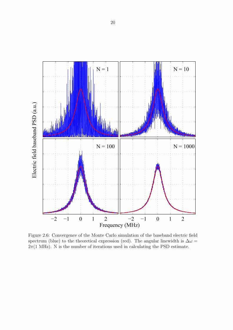
As an exercise, we numerically verify equation (2.30) using a Monte Carlo simu-

lation. We model a flat angular frequency noise spectrum by drawing samples from

a zero-mean Gaussian distribution. These frequency noise samples are integrated in

time, and the cosine of the resultant phase noise is calculated. The PSD of this signal

therefore corresponds to half the baseband spectrum of equation (2.28). Each itera-

tion of this procedure is performed over a finite time T , and therefore yields only an

estimate of the true PSD. If the angular frequency resolution 2π/T is much smaller

than the angular linewidth ∆ω, the mean of this estimate, over many iterations, will

converge to equation (2.28) [44].

Estimates of baseband electric field spectra corresponding to S .φn

(ω) = 2π(1 MHz)

are shown in blue in figure 2.6. As the number of iterations N used in the calculation

is increased, the simulated PSD converges to the true PSD of equation (2.28), shown

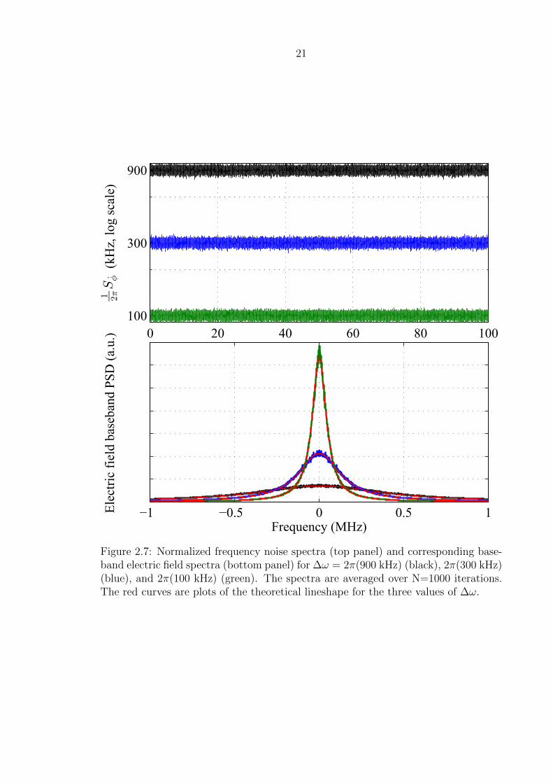
in red. Simulated frequency noise spectra and corresponding baseband lineshapes

for three different values of ∆ω are plotted in figure 2.7, illustrating the relation of

equation (2.29).

2.1.3.3 Fringe Visibility in an FMCW Measurement

We continue or analysis by modifying the chirped electric field in equation (2.1) to

include phase noise,

e(t) = rect

(t− T/2T

)cos

(φ0 + ω0t+

ξt2

2+ φn(t)

), (2.31)

and assume a perfect reflector (R = 1). The photocurrent is therefore given by

i(t) = rect

(t− T/2T

){1 + cos

[(ξτ)t+ ω0τ −

ξτ 2

2+ ∆φn(t, τ)

]}, (2.32)

20

N = 1 N = 10

−2 −1 0 1 2

N = 1000

−2 −1 0 1 2

N = 100

Frequency (MHz)

Elec

tric

field

bas

eban

d PS

D (a

.u.)

Figure 2.6: Convergence of the Monte Carlo simulation of the baseband electric fieldspectrum (blue) to the theoretical expression (red). The angular linewidth is ∆ω =2π(1 MHz). N is the number of iterations used in calculating the PSD estimate.

21

0 20 40 60 80 100100

300

900

−1 −0.5 0 0.5 1

1 2πSφ̇

(kH

z, lo

g sc

ale)

Elec

tric

field

bas

eban

d PS

D (a

.u.)

Frequency (MHz)

Figure 2.7: Normalized frequency noise spectra (top panel) and corresponding base-band electric field spectra (bottom panel) for ∆ω = 2π(900 kHz) (black), 2π(300 kHz)(blue), and 2π(100 kHz) (green). The spectra are averaged over N=1000 iterations.The red curves are plots of the theoretical lineshape for the three values of ∆ω.

22

where ∆φn(t, τ) is the familiar accumulated phase error during time τ . In the noiseless

case, the oscillations (fringes) in the photocurrent extend from 0 to 2. The presence

of phase noise will add jitter to the locations of the peaks and troughs. The ampli-

tude of the fringes, averaged over many scans, is therefore expected to decrease with

increasing phase noise. To quantify this effect, we define the fringe visibility

V ≡ imax − iminimax + imin

, (2.33)

where imax and imin are the photocurrent values at the peaks and troughs, averaged

over many scans. The visibility takes on a value of 1 in the noiseless case, and goes

to zero as the amount of noise increases. Using the identities in equation (2.20), we

write down expressions for the maximum and minimum currents,

imax = 1 + exp

[−σ2

∆φn(τ)

2

], and

imin = 1− exp

[−σ2

∆φn(τ)

2

].

(2.34)

Plugging in equation (2.27) and equation (2.34) into equation (2.33), we arrive at an

expression for the phase-noise-limited visibility [45],

V = exp

(−|τ |∆ω

2

)= exp

(−|τ |τc

), (2.35)

where

τc ≡2

∆ω=

1

π∆ν(2.36)

is the coherence time of the SFL. For delays much shorter than the coherence time,

the visibility decreases linearly with τ . Once τ is comparable to τc, the visibility

drops exponentially. The coherence time is therefore a measure of the longest range

that can be acquired by an FMCW system.

23

2.1.3.4 Spectrum of the FMCW Photocurrent and the SNR

The signal-to-noise ratio (SNR) is more useful in quantifying the effect of phase noise

than the visibility. To determine the SNR we must first calculate the photocurrent

spectrum. We assume a balanced detector and disregard, for now, the rect function

that models the finite chirp bandwidth of the SFL. The photocurrent expression

becomes

i(t) =√R cos

[(ξτ)t+ ω0τ −

ξτ 2

2+ ∆φn(t, τ)

]. (2.37)

Plugging this expression into equation (2.13), we find the autocorrelation,

Ri(u) =R

2〈cos [(ξτ)u+ ∆φn(t, τ)−∆φn(t− u, τ)]〉t

=R

2〈cos [(ξτ)u+ θ(t, τ, u)]〉t

=R

2cos [(ξτ)u] exp

[−σ

2θ(τ, u)

2

],

(2.38)

where

θ(t, τ, u) ≡ ∆φn(t, τ)−∆φn(t− u, τ), (2.39)

and we have assumed that θ(t, τ, u) possesses Gaussian statistics. Taking the FT of

equation (2.38), we find the spectrum of the photocurrent.

Si(ω) =1

4[S◦i (ω − ξτ) + S◦i (ω + ξτ)] , (2.40)

where S◦i (ω) is the baseband spectrum given by

S◦i (ω) = Fu{

exp

[−σ2θ(τ,u)

2

]}. (2.41)

To find the baseband spectrum and the SNR we need to calculate the variance of

θ(t, τ, u). First we derive a useful identity. Let us write down the variance of ∆φn(t, u),

24

as it is defined in equation (2.15),

σ2∆φn(u) =

⟨[φn(t)− φn(t− u)]2

⟩t

= 2σ2φn − 2 〈φn(t)φn(t− u)〉t .

(2.42)

This gives us an expression for the autocorrelation of φn(t),

Rφ(u) = 〈φn(t)φn(t− u)〉t = σ2φn −

σ2∆φn

(u)

2. (2.43)

We plug this result into equation (2.24),

R∆φn(s, u) = 2Rφn(s)−Rφn(s+ u)−Rφn(s− u)

=σ2

∆φn(s+ u)

2+σ2

∆φn(s− u)

2− σ2

∆φn(s)

. (2.44)

We are now in a position to calculate the variance of θ(t, τ, u). Beginning with the

definition in equation (2.15),

σ2θ(τ, u) =

⟨[∆φn(t, τ)−∆φn(t− u, τ)]2

⟩t

=⟨∆φn(t, τ)2 + ∆φn(t− u, τ)2 − 2∆φn(t, τ)∆φn(t− u, τ)

⟩t

= 2σ2∆φn(τ)− 2R∆φn(u, τ).

(2.45)

Plugging in equation (2.44), we arrive at

σ2θ(τ, u) = 2σ2

∆φn(τ) + 2σ2∆φn(u)− σ2

∆φn(u+ τ)− σ2∆φn(u− τ). (2.46)

Using the result of equation (2.27), we write down a final expression for the vari-

ance of θ(t, τ, u),

σ2θ(τ, u) = ∆ω (2τ + 2|u| − |u− τ | − |u+ τ |)

=

4|u|τc

|u| ≤ τ,

4τ

τc|u| > τ.

(2.47)

25

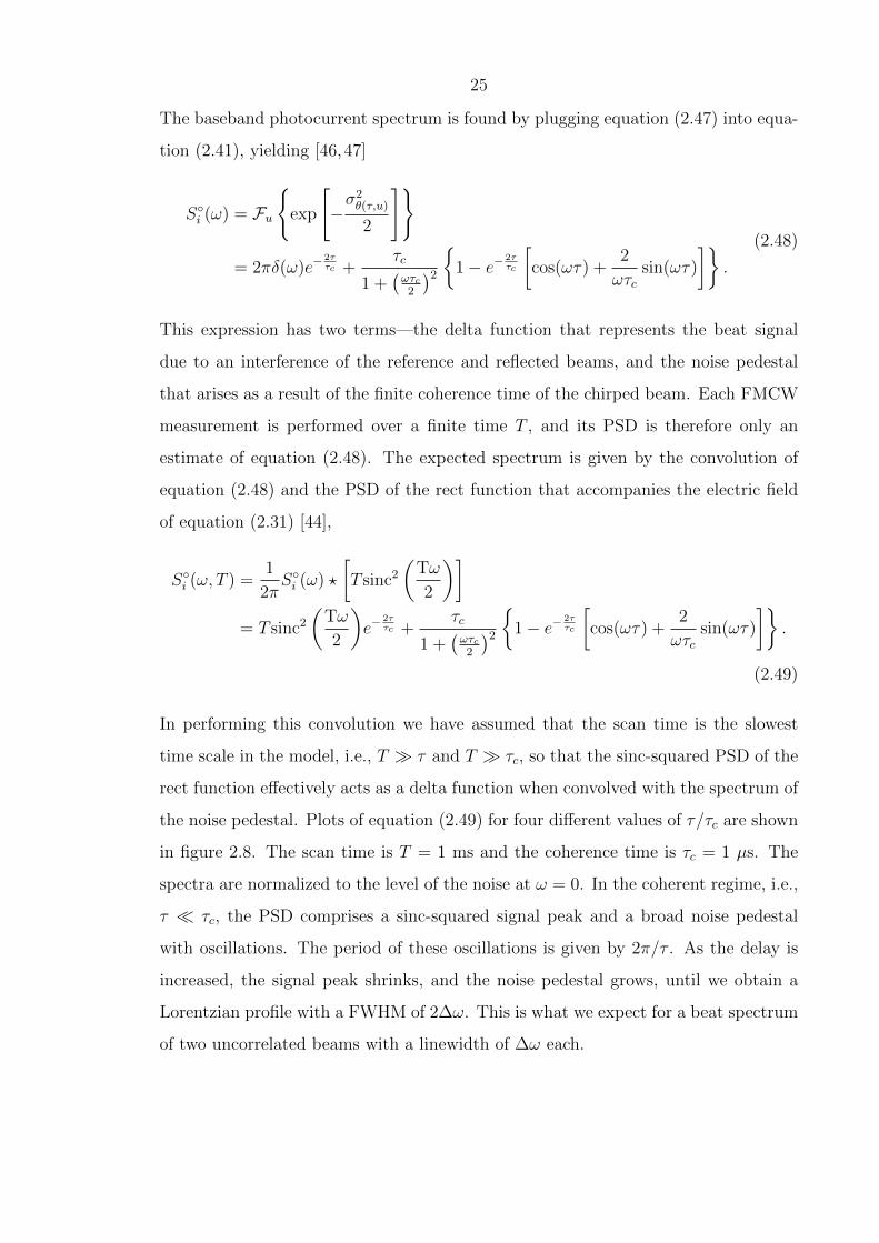
The baseband photocurrent spectrum is found by plugging equation (2.47) into equa-

tion (2.41), yielding [46,47]

S◦i (ω) = Fu{

exp

[−σ2θ(τ,u)

2

]}

= 2πδ(ω)e−2ττc +

τc

1 +(ωτc2

)2

{1− e− 2τ

τc

[cos(ωτ) +

2

ωτcsin(ωτ)

]}.

(2.48)

This expression has two terms—the delta function that represents the beat signal

due to an interference of the reference and reflected beams, and the noise pedestal

that arises as a result of the finite coherence time of the chirped beam. Each FMCW

measurement is performed over a finite time T , and its PSD is therefore only an

estimate of equation (2.48). The expected spectrum is given by the convolution of

equation (2.48) and the PSD of the rect function that accompanies the electric field

of equation (2.31) [44],

S◦i (ω, T ) =1

2πS◦i (ω) ?

[T sinc2

(Tω

2

)]= T sinc2

(Tω

2

)e−

2ττc +

τc

1 +(ωτc2

)2

{1− e− 2τ

τc

[cos(ωτ) +

2

ωτcsin(ωτ)

]}.

(2.49)

In performing this convolution we have assumed that the scan time is the slowest

time scale in the model, i.e., T � τ and T � τc, so that the sinc-squared PSD of the

rect function effectively acts as a delta function when convolved with the spectrum of

the noise pedestal. Plots of equation (2.49) for four different values of τ/τc are shown

in figure 2.8. The scan time is T = 1 ms and the coherence time is τc = 1 µs. The

spectra are normalized to the level of the noise at ω = 0. In the coherent regime, i.e.,

τ � τc, the PSD comprises a sinc-squared signal peak and a broad noise pedestal

with oscillations. The period of these oscillations is given by 2π/τ . As the delay is

increased, the signal peak shrinks, and the noise pedestal grows, until we obtain a

Lorentzian profile with a FWHM of 2∆ω. This is what we expect for a beat spectrum

of two uncorrelated beams with a linewidth of ∆ω each.

26

−30−20

−100

1020

3040

τ/τc = 0.3 τ/τ

c = 1

−10 0 10

τ/τc = 10

−10 0 10−30−20

−100

1020

3040

τ/τc = 3

Frequency (MHz)

Phot

ocur

rent

bas

eban

d PS

D re

lativ

e to

noi

se (d

Brn

/Hz)

Figure 2.8: Baseband FMCW photocurrent spectra for four different values of τ/τc,normalized to zero-frequency noise levels. The scan time is T = 1 ms and the coher-ence time is τc = 1 µs.

27

10−2 10−1 100 101−80

−60

−40

−20

0

20

40

60

80

τ/τc

Sign

al to

noi

se ra

tio (d

B)

T/τc = 102

T/τc = 103

T/τc = 104

Figure 2.9: FMCW SNR as a function of τ/τc for three different values of T/τc

28

The SNR is readily calculated from equation (2.49), and is given in decibel units

by

SNRdB = 10 log10

Tτi× 1

e2τ/τc −(

1 + 2ττc

) . (2.50)

A plot of the SNR versus τ/τc is shown in figure 2.9 for three different values of

T/τc. In the coherent regime, the SNR decreases at 20 dB/decade with τ/τc, and

drops sharply for τ > τc. This is consistent with the rapid decrease in visibility

for delays longer than the coherence time, as predicted by equation (2.35). As the

current analysis shows, the visibility is not the full story—even low fringe visibilities

can result in a decent SNR, provided that the scan time T is long enough.

2.1.3.5 Phase-Noise-Limited Accuracy

The axial resolution of an FMCW system, ∆z = c/2B, quantifies its ability to tell

apart closely-spaced scatterers. If we assume that the beam only encounters a single

scatterer, as it would in a profilometry application, then the relevant system metric

is the accuracy—the deviation of the measured target delay τm from the true target

delay τ . We briefly consider statistical properties of the accuracy using the phase

noise model developed above.

The instantaneous photocurrent frequency in a single-scatterer FMCW experi-

ment is given by a derivative of the cosine phase in equation (2.37),

ωPD(t) = ξτ +d

dt∆φn(t, τ). (2.51)

The target delay is calculated from an average of the photocurrent frequency over the

scan time T ,

ξτm =1

T

∫ T

0

ωPD(t) = ξτ +∆φn(T, τ)−∆φn(0, τ)

T. (2.52)

29

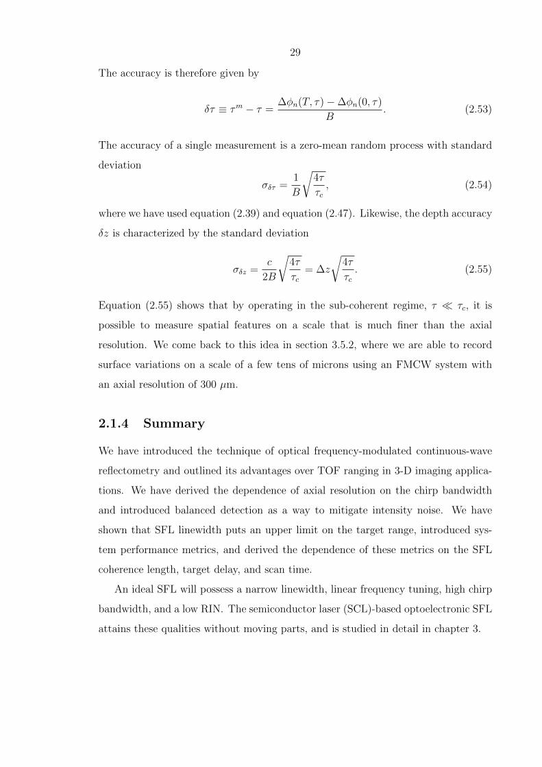
The accuracy is therefore given by

δτ ≡ τm − τ =∆φn(T, τ)−∆φn(0, τ)

B. (2.53)

The accuracy of a single measurement is a zero-mean random process with standard

deviation

σδτ =1

B

√4τ

τc, (2.54)

where we have used equation (2.39) and equation (2.47). Likewise, the depth accuracy

δz is characterized by the standard deviation

σδz =c

2B

√4τ

τc= ∆z

√4τ

τc. (2.55)

Equation (2.55) shows that by operating in the sub-coherent regime, τ � τc, it is

possible to measure spatial features on a scale that is much finer than the axial

resolution. We come back to this idea in section 3.5.2, where we are able to record

surface variations on a scale of a few tens of microns using an FMCW system with

an axial resolution of 300 µm.

2.1.4 Summary

We have introduced the technique of optical frequency-modulated continuous-wave

reflectometry and outlined its advantages over TOF ranging in 3-D imaging applica-

tions. We have derived the dependence of axial resolution on the chirp bandwidth

and introduced balanced detection as a way to mitigate intensity noise. We have

shown that SFL linewidth puts an upper limit on the target range, introduced sys-

tem performance metrics, and derived the dependence of these metrics on the SFL

coherence length, target delay, and scan time.

An ideal SFL will possess a narrow linewidth, linear frequency tuning, high chirp

bandwidth, and a low RIN. The semiconductor laser (SCL)-based optoelectronic SFL

attains these qualities without moving parts, and is studied in detail in chapter 3.