Chapter 2

Refrigerated Condensers

Karen Schaffner

Kevin Bradley

David Randall

RTI International

Research Triangle Park, NC 27709

John L. Sorrels

Air Economics Group, OAQPS

U.S. Environmental Protection Agency

Research Triangle Park, NC 27711

November 2017

i

Contents

2.1 Introduction ......................................................................................................................... 2-1

2.1.1 System Efficiencies and Performance .................................................................... 2-1

2.2 Process Description ............................................................................................................. 2-1

2.2.1 VOC Condensers ..................................................................................................... 2-3

2.2.2 Refrigeration Unit ................................................................................................... 2-4

2.2.3 Auxiliary Equipment ............................................................................................... 2-5

2.3 Design Procedures .............................................................................................................. 2-5

2.3.1 Estimating Condensation Temperature ................................................................... 2-6

2.3.2 VOC Condenser Heat Load .................................................................................... 2-8

2.3.3 Condenser Size...................................................................................................... 2-11

2.3.4 Coolant Flow Rate ................................................................................................ 2-12

2.3.5 Refrigeration Capacity .......................................................................................... 2-13

2.3.6 Recovered VOC .................................................................................................... 2-13

2.3.7 Auxiliary Equipment ............................................................................................. 2-13

2.3.8 Alternate Design Procedure .................................................................................. 2-14

2.4 Estimating Total Capital Investment ................................................................................ 2-14

2.4.1 Equipment Costs for Packaged Solvent Vapor Recovery Systems ...................... 2-15

2.4.2 Equipment Costs for Nonpackaged (Custom) Solvent Vapor Recovery

Systems ................................................................................................................. 2-18

2.4.3 Equipment Costs for Gasoline Vapor Recovery Systems..................................... 2-19

2.4.4 Installation Costs ................................................................................................... 2-20

2.5 Estimating Total Annual Cost ....................................................................................... 2-2221

2.5.1 Direct Annual Costs .............................................................................................. 2-22

2.5.2 Indirect Annual Costs ........................................................................................... 2-23

2.5.3 Recovery Credit .................................................................................................... 2-24

2.5.4 Total Annual Cost ................................................................................................. 2-24

2.6 Example Problem 1 ........................................................................................................... 2-24

2.6.1 Required Information for Design .......................................................................... 2-24

2.6.2 Equipment Sizing .................................................................................................. 2-25

2.6.3 Equipment Costs ................................................................................................... 2-28

2.6.4 Total Annual Cost ................................................................................................. 2-29

2.7 Example Problem 2 ........................................................................................................... 2-31

2.7.1 Required Information for Design .......................................................................... 2-31

ii

2.8 Acknowledgements ........................................................................................................... 2-31

References .................................................................................................................................. 2-32

Appendix A Properties of Selected Compounds ......................................................................... 2-34

Appendix B Documentation for Gasoline Vapor Recovery System Cost Data ......................... 2-38

2-1

2.1 Introduction

Condensers in use today may fall in either of two categories: refrigerated or non-

refrigerated. Non-refrigerated condensers are widely used as raw material, product, and/or

solvent recovery devices in chemical process industries. They are frequently used prior to control

devices (e.g., incinerators or absorbers). Refrigerated condensers are used as air pollution control

devices for treating emission streams with high VOC concentrations (usually > 5,000 ppmv) in

applications involving gasoline bulk terminals, storage, etc. Condenser control technology is

unique in that it not only reduces emissions to the atmosphere but also captures or recovers

VOCs, potentially for additional use.

Condensation is a separation technique in which one or more volatile components of a

vapor mixture are separated from the remaining vapors through saturation followed by a phase

change. The phase change from gas to liquid can be achieved in two ways: (a) the system

pressure can be increased at a given temperature, or (b) the temperature may be lowered at a

constant pressure. In a two-component system where one of the components is noncondensible

(e.g., air), condensation occurs at dew point (saturation) when the partial pressure of the volatile

compound is equal to its vapor pressure. The more volatile a compound is (e.g., the lower the

normal boiling point), the larger the amount that can remain as vapor at a given temperature;

hence the lower the temperature required for saturation (condensation). Refrigeration is often

employed to obtain the low temperatures required for acceptable removal efficiencies. This

chapter is limited to the evaluation of refrigerated condensation at constant (atmospheric)

pressure.

2.1.1 System Efficiencies and Performance

The removal efficiency of a condenser is dependent on the emission stream

characteristics including the nature of the VOC in question (vapor pressure/temperature

relationship), VOC concentration, and the type of coolant used.1 Any component of any vapor

mixture can be condensed if brought to a low enough temperature and allowed to come to

equilibrium. Figure 2.1 shows the vapor pressure dependence on temperature for selected

compounds (Erikson, 1980). A condenser cannot lower the inlet concentration to levels below

the saturation concentration at the coolant temperature. Removal efficiencies of approximately

50 to 90 percent can be achieved with coolants such as chilled water and brine solutions, and

removal efficiencies above 90 percent can be achieved with ammonia, liquid nitrogen,

chlorofluorocarbons, hydrochlorofluorocarbons, or hydrofluorocarbons, depending on the VOC

composition and concentration level of the emission stream.

2.2 Process Description

Figure 2.2 depicts a typical configuration for a refrigerated surface condenser system as

an emission control device. The basic equipment required for a refrigerated condenser system

includes a VOC condenser, a refrigeration unit(s), and auxiliary equipment (e.g., precooler,

recovery/storage tank, pump/blower, and piping).

1 Organic hazardous air pollutants (HAPs) are considered a subset of VOC compounds.

2-2

Figure 2.1: Vapor Pressures of Selected Compounds vs. Temperature (Erikson, 1980)

Figure 2.2: Schematic Diagram for a Refrigerated Condenser System

2-3

2.2.1 VOC Condensers

The two most common types of condensers used are surface and contact condensers

(Vatavuk and Neveril, 1983). In surface condensers, the coolant does not contact the gas stream.

Most surface condensers in refrigerated systems are the shell and tube type (see Figure 2.3)

(McCabe and Smith, 1976). Shell and tube condensers circulate the coolant through tubes. The

VOCs condense on the outside of the tubes (i.e., within the shell). Plate and frame type heat

exchangers are also used as condensers in refrigerated systems. In these condensers, the coolant

and the vapor flow separately over thin plates. In either design, the condensed vapor forms a film

on the cooled surface and drains away to a collection tank for storage, reuse, or disposal.

In contrast to surface condensers where the coolant does not contact either the vapors or

the condensate, contact condensers cool the vapor stream by spraying either a liquid at ambient

temperature or a chilled liquid directly into the gas stream.

Spent coolant containing the VOCs from contact condensers usually cannot be reused

directly and can be a waste disposal problem. Additionally, VOCs in the spent coolant cannot be

directly recovered without further processing. Since the coolant from surface condensers does

not contact the vapor stream, it is not contaminated and can be recycled in a closed loop. Surface

condensers also allow for direct recovery of VOCs from the gas stream. This chapter addresses

the design and costing of refrigerated surface condenser systems only.

Figure 2.3: Schematic Diagram of a Shell and Tube Surface Condenser (McCabe and Smith, 1976)

2-4

2.2.2 Refrigeration Unit

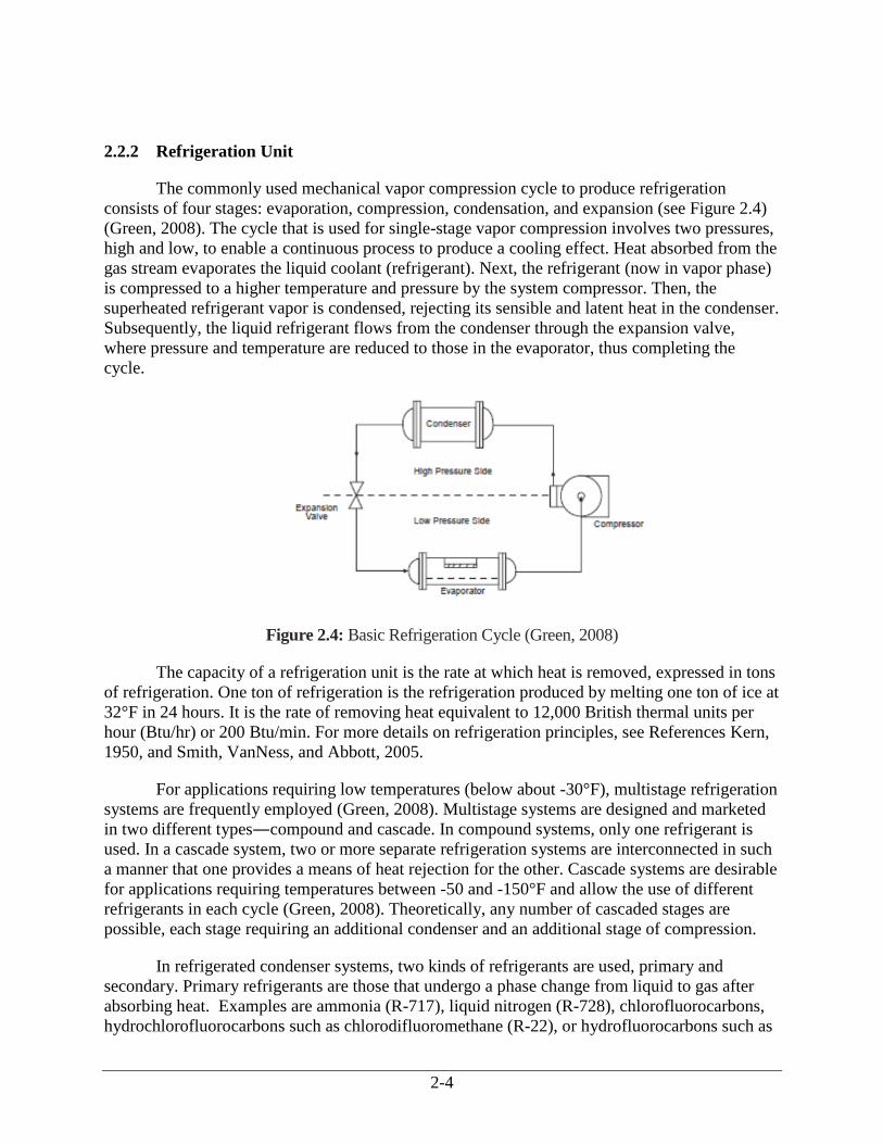
The commonly used mechanical vapor compression cycle to produce refrigeration

consists of four stages: evaporation, compression, condensation, and expansion (see Figure 2.4)

(Green, 2008). The cycle that is used for single-stage vapor compression involves two pressures,

high and low, to enable a continuous process to produce a cooling effect. Heat absorbed from the

gas stream evaporates the liquid coolant (refrigerant). Next, the refrigerant (now in vapor phase)

is compressed to a higher temperature and pressure by the system compressor. Then, the

superheated refrigerant vapor is condensed, rejecting its sensible and latent heat in the condenser.

Subsequently, the liquid refrigerant flows from the condenser through the expansion valve,

where pressure and temperature are reduced to those in the evaporator, thus completing the

cycle.

Figure 2.4: Basic Refrigeration Cycle (Green, 2008)

The capacity of a refrigeration unit is the rate at which heat is removed, expressed in tons

of refrigeration. One ton of refrigeration is the refrigeration produced by melting one ton of ice at

32°F in 24 hours. It is the rate of removing heat equivalent to 12,000 British thermal units per

hour (Btu/hr) or 200 Btu/min. For more details on refrigeration principles, see References Kern,

1950, and Smith, VanNess, and Abbott, 2005.

For applications requiring low temperatures (below about -30°F), multistage refrigeration

systems are frequently employed (Green, 2008). Multistage systems are designed and marketed

in two different types―compound and cascade. In compound systems, only one refrigerant is

used. In a cascade system, two or more separate refrigeration systems are interconnected in such

a manner that one provides a means of heat rejection for the other. Cascade systems are desirable

for applications requiring temperatures between -50 and -150°F and allow the use of different

refrigerants in each cycle (Green, 2008). Theoretically, any number of cascaded stages are

possible, each stage requiring an additional condenser and an additional stage of compression.

In refrigerated condenser systems, two kinds of refrigerants are used, primary and

secondary. Primary refrigerants are those that undergo a phase change from liquid to gas after

absorbing heat. Examples are ammonia (R-717), liquid nitrogen (R-728), chlorofluorocarbons,

hydrochlorofluorocarbons such as chlorodifluoromethane (R-22), or hydrofluorocarbons such as

2-5

R-410A or 1,1,1,2-Tetrafluoroethane (R-134a). Concerns about CFCs and HCFCs causing

depletion of the ozone layer prompted development of HFCs, and recent concerns about HFCs

being potent greenhouse gases are further prompting development of systems using alternate

refrigerants (EPA, 2001, and EPA, 2015).

Secondary refrigerants such as brine solutions act only as heat carriers and remain in

liquid phase. Conventional systems use a closed primary refrigerant loop that cools the

secondary loop through the heat transfer medium in the evaporator. The secondary heat transfer

fluid is then pumped to a VOC vapor condenser where it is used to cool the air/VOC vapor

stream. In some applications, however, the primary refrigeration fluid is directly used to cool the

vapor stream.

2.2.3 Auxiliary Equipment

As shown in Figure 2.2, some applications may require auxiliary equipment such as

precoolers, recovery/storage tanks, pumps/blowers, and piping.

If water vapor is present in the treated gas stream or if the VOC has a high freezing point

(e.g., benzene), ice or frozen hydrocarbons may form on the condenser tubes or plates. This will

reduce the heat transfer efficiency of the condenser and thereby reduce the removal efficiency.

Formation of ice will also increase the pressure drop across the condenser. In such cases, a

precooler may be needed to condense the moisture prior to the VOC condenser. This precooler

would bring the temperature of the stream down to approximately 35 to 40°F, effectively

removing the moisture from the gas. Alternatively, an intermittent heating cycle can be used to

melt away ice build-up. This may be accomplished by circulating ambient temperature brine

through the condenser or by the use of radiant heating coils. If a system is not operated

continuously, the ice can also be removed by circulating ambient air.

A VOC recovery tank for temporary storage of condensed VOC prior to reuse,

reprocessing, or transfer to a larger storage tank may be necessary in some cases. Pumps and

blowers are typically used to transfer liquid (e.g., coolant or recovered VOC) and gas streams,

respectively, within the system.

2.3 Design Procedures

In this section, two procedures are presented for designing (sizing) refrigerated surface

condenser systems to remove VOC from air/VOC mixtures. With the first procedure presented,

one calculates the condenser exit temperature needed to obtain a given VOC recovery efficiency.

In the second procedure, which is the inverse of the first, the exit temperature is given and the

recovery efficiency corresponding to it is calculated.

The first procedure depends on knowledge of the following parameters:

1. Volumetric flow rate of the VOC-containing gas stream;

2. Inlet temperature of the gas stream;

3. Concentration and composition of the VOC in the gas stream;

2-6

4. Required removal efficiency of the VOC;

5. Moisture content of the emission stream; and

6. Properties of the VOC (assuming the VOC is a pure compound):

Heat of condensation,

Heat capacity, and

Vapor pressure.

The design of a refrigerated condenser system requires determination of the VOC

condenser size and the capacity of the refrigeration unit. For a given VOC removal efficiency,

the condensation temperature and the heat load need to be calculated to determine these

parameters. The data necessary to perform the sizing procedures as well as the variable names

and their respective units are listed in Table 2.1.

Table 2.1: Required Input Data

Data Variable Name Units

Inlet Stream Flow Rate Qin scfm (at 77 °F; 1 atm)

Inlet Stream Temperature Tin °F

VOC Inlet Volume Fraction yVOC,in Volume fraction

Required VOC Removal Efficiency η Fractional (volume)

Antoine Equation Constantsa A, B, C ―

Heat of Condensation of the VOCa ∆H Btu/lb-mole

Heat Capacity of the VOCa Cp,VOC Btu/lb-mole-°F

Specific Heat of the Coolant Cp,cool Btu/lb-°F

Heat Capacity of Air Cp,air Btu/lb-mole-°F

aSee Appendix A for these properties of selected organic compounds.

The steps outlined below for estimating condensation temperature and the heat load apply

to a two-component mixture (VOC/air) in which one of the two components is considered to be

noncondensible (air). The VOC component is assumed to consist of a single compound. Also,

the emission stream is assumed to be free of moisture. The calculations are based on the

assumptions of ideal gas and ideal solution to simplify the sizing procedures. For a more rigorous

analysis, see Reference Kern, 1950.

2.3.1 Estimating Condensation Temperature

The temperature necessary to condense the required amount of VOC must be estimated to

determine the heat load. The first step is to determine the VOC concentration at the outlet of the

condenser for a given removal efficiency. This is calculated by first determining the partial

pressure of the VOC at the outlet, PVOC. Assuming that the ideal gas law applies, PVOC is given

by:

2-7

MM

MP

eredcovreVOCin

outVOC

VOC

,

,760

(2.1)

where:

PVOC = partial pressure of the VOC in the exit stream (mm Hg)

Min = moles in the inlet stream (moles per hour, moles/hr)

MVOC,out = moles of VOC in the outlet stream (moles/hr)

MVOC,recovered = moles of VOC condensed, or recovered (moles/hr)

The condenser is assumed to operate at a constant pressure of one atmosphere (760 mm Hg).

However:

1, inVOCVOC,out

MM (2.2)

where:

MVOC,in = moles of VOC in the inlet stream (moles/hr)

η = removal efficiency of the condenser system (fractional)

and

VOC,inininVOCyMM

, (2.3)

where:

yVOC,in = volume fraction of VOC in inlet stream.

The removal efficiency, η, can also be defined as “moles VOC recovered / moles VOC in inlet:”

inletinVOCmoles

recoveredVOCmoles

or:

in,VOC

eredcovre,VOC

M

M (2. 4)

Rearranging Equation 2.4, we obtain:

in,VOCeredcovre,VOC

MM (2.5)

After substituting these variables in Equation 2.1, we obtain:

2-8

VOC,in

VOC,in

VOCy

yP

1

1760 (2.6)

At the condenser outlet, the VOC in the gas stream is assumed to be at equilibrium with

the VOC condensate. At equilibrium, the partial pressure of the VOC in the gas stream is equal

to its vapor pressure at that temperature assuming the condensate is pure VOC (i.e., vapor

pressure PVOC). Therefore, by determining the temperature at which this condition occurs, the

condensation temperature can be specified. This calculation is based on the Antoine equation that

defines the relationship between vapor pressure and temperature for a particular compound:

CT

BAP

con

VOC

10

log (2.7)

where:

Tcon = condensation temperature (degrees Celsius, or °C)

A, B, C = VOC-specific constants pertaining to temperature expressed in °C and pressure

in millimeters of mercury (mm Hg) (see Appendix A, Table A-2)

Rearranging and solving for Tcon in degrees Fahrenheit (ºF):

328.1)(log

10

C

PA

BT

VOC

con (2.8)

The calculation methods for a gas stream containing multiple VOCs are complex,

particularly when there are significant departures from the ideal behavior of gases and liquids.

However, the temperature necessary for condensation of a mixture of VOCs can be estimated by

the weighted average of the temperatures necessary to condense each VOC in the gas stream at a

concentration equal to the total VOC concentration (Erikson, 1980).

2.3.2 VOC Condenser Heat Load

Condenser heat load is the amount of heat that must be removed from the inlet stream to

attain the specified removal efficiency. It is determined from an energy balance, taking into

account the enthalpy change due to the temperature change of the VOC, the enthalpy change due

to the condensation of the VOC, and the enthalpy change due to the temperature change of the

air. Enthalpy change due to the presence of moisture in the inlet gas stream is neglected in the

following analysis.

For the purpose of this estimation, it is assumed that the total heat load on the system is

equal to the VOC condenser heat load. Realistically, when calculating refrigeration capacity

requirements for low temperature cooling units, careful consideration should be given to the

process line losses and heat input of the process pumps. Refrigeration unit capacities are

typically rated in terms of net output and do not reflect any losses through process pumps or

process lines.

2-9

First, the number of lb-moles of VOC per hour in the inlet stream must be calculated by

the following expression:

60392

,,

inVOC

in

inVOCy

QM (2.9)

where:

MVOC,in = moles of VOC in the inlet stream, lb-moles/hr

Qin = volume flow rate in standard ft3/min (scfm)

392 = volume (ft3) occupied by one lb-mole of gas at standard conditions (77°F and 1

atm)

60 = conversion from minutes to hours (min/hr)

The number of lb-moles of VOC per hour in the outlet gas stream is calculated using Equation

2.2. Finally, the number of lb-moles of VOC per hour that are condensed (or recovered) is

calculated as follows:

outVOCinVOCrecoveredVOCMMM

,,, (2.10)

The condenser heat load is calculated by the following equation:

nonconunconconloadHHHH (2.11)

where:

Hload = condenser heat load (Btu/hr)

∆Hcon = enthalpy change associated with the condensed VOC (Btu/hr)

∆Huncon = enthalpy change associated with the uncondensed VOC (Btu/hr)

∆Hnoncon = enthalpy change associated with the noncondensible air (Btu/hr)

The change in enthalpy of the condensed VOC is calculated as follows:

coninVOCpVOCeredcovreVOCcon

TTCHMH ,, (2.12)

where:

∆HVOC = molar heat of condensation of the VOC (Btu/lb-mole)

Cp,VOC = molar heat capacity of the VOC (Btu/lb-mole-ºF)

Tin = inlet stream temperature (°F)

Tcon = condensation temperature (°F)

2-10

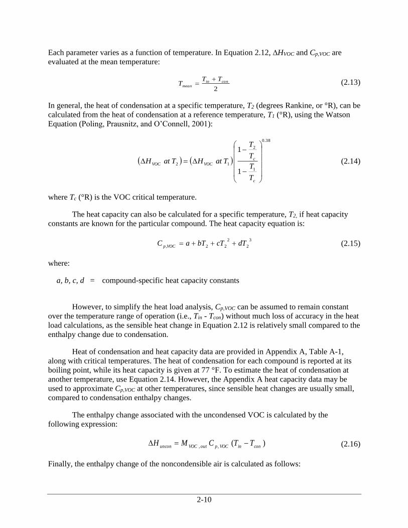
Each parameter varies as a function of temperature. In Equation 2.12, ∆HVOC and Cp,VOC are

evaluated at the mean temperature:

2

conin

mean

TTT

(2.13)

In general, the heat of condensation at a specific temperature, T2 (degrees Rankine, or °R), can be

calculated from the heat of condensation at a reference temperature, T1 (°R), using the Watson

Equation (Poling, Prausnitz, and O’Connell, 2001):

38.0

1

2

12

1

1

c

c

VOCVOC

T

T

T

T

TatHTatH (2.14)

where Tc (°R) is the VOC critical temperature.

The heat capacity can also be calculated for a specific temperature, T2, if heat capacity

constants are known for the particular compound. The heat capacity equation is:

3

2

2

22,dTcTbTaC

VOCp (2.15)

where:

a, b, c, d = compound-specific heat capacity constants

However, to simplify the heat load analysis, Cp,VOC can be assumed to remain constant

over the temperature range of operation (i.e., Tin - Tcon) without much loss of accuracy in the heat

load calculations, as the sensible heat change in Equation 2.12 is relatively small compared to the

enthalpy change due to condensation.

Heat of condensation and heat capacity data are provided in Appendix A, Table A-1,

along with critical temperatures. The heat of condensation for each compound is reported at its

boiling point, while its heat capacity is given at 77 °F. To estimate the heat of condensation at

another temperature, use Equation 2.14. However, the Appendix A heat capacity data may be

used to approximate Cp,VOC at other temperatures, since sensible heat changes are usually small,

compared to condensation enthalpy changes.

The enthalpy change associated with the uncondensed VOC is calculated by the

following expression:

)(,, coninVOCpoutVOCuncon

TTCMH (2.16)

Finally, the enthalpy change of the noncondensible air is calculated as follows:

2-11

)(60392

,, coninairpinVOC

in

nonconTTCM

QH

(2.17)

where Cp,air is the specific heat of air. In both Equations 2.16 and 2.17, the Cp’s are evaluated at

the mean temperature, as given by Equation 2.13.

2.3.3 Condenser Size

Condensers are sized based on the heat load, the logarithmic mean temperature difference

between the emission and coolant streams, and the overall heat transfer coefficient. The overall

heat transfer coefficient, U, can be estimated from individual heat transfer coefficients of the gas

stream and the coolant. The overall heat transfer coefficients for tubular heat exchangers where

organic solvent vapors in noncondensible gas are condensed on the shell side and water/brine is

circulated on the tube side typically range from 20 to 60 Btu/hr-ft2-°F according to Perry’s

Chemical Engineers’ Handbook (Green, 2008). To simplify the calculations, a single U value

may be used to size these condensers. This approximation is acceptable for purposes of making

study-level (±30% accuracy) cost estimates.

Accordingly, an estimate of 20 Btu/hr-ft2-°F can be used to obtain a conservative

estimate of condenser size (i.e., more likely to overstate the required condenser surface area).

The following equation is used to determine the required heat transfer area:

lm

load

conTU

HA

(2.18)

where:

Acon = condenser surface area (ft2)

U = overall heat transfer coefficient (Btu/hr-ft2-°F)

∆Tlm = logarithmic mean temperature difference (°F).

While not all condensing units will experience fouling, for some applications of

condensers, future, continued operation may result in fouling of the condenser surface areas, and

facilities often account for this in the original condenser design by including a fouling factor in

the overall heat transfer coefficient.2, 3 Because fouling reduces heat transfer, use of a fouling

factor reduces the overall heat transfer coefficient and thereby increases the surface area

estimated for the condensing unit. This overall heat transfer coefficient that accounts for fouling

is sometimes referred to as “Udirty” or “Dirty U.” The fouling factor depends on the materials of

construction, the VOC condensed and other pollutants present, and the type of coolant used. The

2 Ulhrich provides the overall heat transfer coefficient equation, including use of fouling coefficients. Uhlrich, G.,

1984. A Guide to Chemical Engineering Process Design and Economics. Wiley & Sons, Inc., New York. 3 Perry’s provides typical overall heat transfer coefficients, see Table 10-10. Perry’s, 1984. Perry’s Chemical

Engineers’ Handbook, 6th Edition. McGraw-Hill Book Company, New York.

2-12

use of relatively lower values of U, such as the estimate for Eqn. 2.18 above, could provide some

allowance for fouling in the design and cost estimation for condensers.

The logarithmic mean temperature difference is calculated by the following equation,

which is based on the use of a countercurrent flow condenser:

incoolcon

outcoolin

incoolconoutcoolin

lm

TT

TT

TTTTT

,

,

,,

ln

(2.19)

where:

Tcool,in = coolant inlet temperature (°F)

Tcool,out = coolant outlet temperature (°F).

The temperature difference (“approach”) at the condenser exit can be assumed to be

15°F. In other words, the coolant inlet temperature, Tcool,in, will be 15°F less than the calculated

condensation temperature, Tcon. Also, the temperature rise of the coolant is specified as 25°F.

(These two temperatures―the condenser approach and the coolant temperature rise―reflect

good design practice that, if used, will result in an acceptable condenser size.) Therefore, the

following equations can be applied to determine the coolant inlet and outlet temperature:

FTTconincool

15, (2.20)

FTTincooloutcool

25,, (2.21)

2.3.4 Coolant Flow Rate

The heat removed from the emission stream is transferred to the coolant. By a simple

energy balance, the flow rate of the coolant can be calculated as follows:

)(

,,, incooloutcoolcoolp

load

coolTTC

HW

(2.22)

where:

Wcool = coolant flow rate (lb/hr)

Cp,cool = coolant specific heat (Btu/lb-°F)

Cp,cool will vary according to the type of coolant used. For a 50:50 (volume %) mixture of

ethylene glycol and water, Cp,cool is approximately 0.65 Btu/lb-°F. The specific heat of brine (salt

water), another commonly used coolant, is approximately 1.0 Btu/lb-°F.

2-13

2.3.5 Refrigeration Capacity

The refrigeration unit is assumed to supply the coolant at the required temperature to the

condenser. The required refrigeration capacity is calculated by converting the condenser heat

load from Btu/hr to tons of refrigeration as follows:

000,12

loadH

R (2.23)

where:

12,000 = conversion to refrigeration tons (Btu/ton)

Again, as explained in section 2.3.2, Hload does not include any heat losses.

2.3.6 Recovered VOC

The mass of VOC recovered in the condenser can be calculated using the following

expression:

VOCeredcovre,VOCeredcovre,VOCMWMW (2.24)

where:

WVOC,recovered = mass of VOC recovered (or condensed) (lb/hr)

MWVOC = molecular weight of the VOC (lb/lb-mole)

2.3.7 Auxiliary Equipment

As noted previously, the auxiliary equipment for a refrigerated surface condenser system

may include:

precooler,

recovered VOC storage tank,

pumps/blowers, and

piping/ductwork.

If water vapor is present in the treated gas stream, a precooler may be needed to remove

moisture to prevent ice from forming in the VOC condenser. Sizing of a precooler is influenced

by the moisture concentration and the temperature of the emission stream. As discussed in

Section 2.2.3, a precooler may not be necessary for intermittently operated refrigerated surface

condenser systems where the ice will have time to melt between successive operating periods.

If a precooler is required, a typical operating temperature is 35 to 40°F. At this

temperature, almost all of the water vapor present will be condensed without danger of freezing.

These condensation temperatures roughly correspond to a removal efficiency range of 70 to 80

2-14

percent if the inlet stream is saturated with water vapor at 77°F. The design procedure outlined in

the previous sections for a VOC condenser can be used to size a precooler, based on the

psychrometric chart for the air-water vapor system (Green, 2008).

Storage/recovery tanks are used to store the condensed VOC when direct recycling is not

a suitable option. The size of these tanks is determined from the amount of VOC condensate to

be collected and the amount of time necessary before unloading. Sizing of pumps and blowers is

based on the liquid and gas flow rates, respectively, as well as the system pressure drop between

the inlet and outlet. Sizing of the piping and ductwork (length and diameter) primarily depends

upon the stream flow rate, duct/pipe velocity, available space, and system layout.

2.3.8 Alternate Design Procedure

In some applications, it may be desirable to size and cost a refrigerated condenser system

that will use a specific coolant and provide a particular condensation temperature. The design

procedure to be implemented in such a case would essentially be the same as the one presented

in this section except that instead of calculating the condenser exit temperature needed to obtain

a specified VOC recovery efficiency, the exit temperature is given and the corresponding

recovery efficiency is calculated.

The initial calculation would be to estimate the partial (i.e., vapor) pressure of the VOC at

the given condenser exit temperature, Tcon, using Equation 2.7. Next, calculate η using Equation

2.25, by rearranging Equation 2.6:

VOCinVOC

VOCinVOC

Py

Py

760

760

,

, (2.25)

Finally, substitute the calculated PVOC into this equation to obtain η. In the remainder of

the calculations to estimate condenser heat load, refrigeration capacity, coolant flow rate, etc.,

follow the procedure presented in Sections 2.3.2 through 2.3.7.

In future application and operation of the condenser, if process changes result in raw

material, product, or solvent VOC changes; VOC concentration changes; volumetric flowrate

changes; or process temperature changes, the removal or recovery efficiency achieved may differ

from the original VOC design efficiency.

2.4 Estimating Total Capital Investment

This section presents the procedures and data necessary for estimating capital costs for

refrigerated surface condenser systems in solvent vapor recovery and gasoline vapor recovery

applications. Costs for packaged and nonpackaged solvent vapor recovery systems are presented

in Sections 2.4.1 and 2.4.2, respectively. Costs for packaged gasoline vapor recovery systems are

described in Section 2.4.3. Costs are calculated based on the design/sizing procedures discussed

in Section 2.3.

Total capital investment, TCI, includes equipment cost, EC, for the entire refrigerated

condenser unit, auxiliary equipment costs, taxes, freight charges, instrumentation, and direct and

2-15

indirect installation costs. All costs in this chapter are presented in 2014 dollars (2014$). The

costs were escalated from 1990 dollars using a ratio of the years' annual composite Chemical

Engineering Plant Cost Indices (CEPCI). A ratio of annual CEPCI for 2014 and 1990 results in

an escalation factor of 1.611 (i.e., 576.1/357.6) (Lozowski, 2015, and Vatavuk, 2002). Typically,

it is more common to perform this kind of escalation when the difference between the years is

small (i.e., 5 or less) because emerging technologies and practices can increase the inaccuracy of

a simple ratio.

For these control systems, the total capital investment is a battery limit cost estimate and

does not include the provisions for bringing utilities, services, or roads to the site; the backup

facilities; the land; the working capital; the research and development required; or the process

piping and instrumentation interconnections that may be required in the process generating the

waste gas. These costs are based on new plant installations; no retrofit cost considerations are

included. The retrofit cost factors are so site specific that no attempt has been made to provide

them.

The expected accuracy of the cost estimates presented in this chapter is ±30 percent (i.e.,

“study” estimates). It must be kept in mind that even for a given application, design and

manufacturing procedures vary from vendor to vendor, so costs may vary.

In the next two sections, equipment costs are presented for packaged and nonpackaged

(custom) solvent vapor recovery systems, respectively. With the packaged systems, the

equipment cost is factored from the refrigeration unit cost; with the custom systems, the

equipment cost is determined as the sum of the costs of the individual system components. It

should be noted that any adjustments for fouling, if made, will not affect the cost estimates for

the packaged recovery systems. The cost equations for these systems are based on refrigeration

and temperature as variables, and surface area is not a variable. Surface area is a variable in the

custom systems equations, and effects from fouling are explicitly accounted for. Finally,

equipment costs for packaged gasoline vapor recovery systems are given in Section 2.4.3.

2.4.1 Equipment Costs for Packaged Solvent Vapor Recovery Systems

Vendors were asked to provide refrigerated unit cost estimates for a wide range of

applications. The equations shown below for refrigeration unit equipment costs, ECr, are

multivariable regressions of data provided by two vendors and are only valid for the ranges listed

in Table 2.2 (Sisk, 1991, and Waldrop and Sardo, 1990). In this table, the capacity range of

refrigeration units for which cost data were available are shown as a function of temperature.

2-16

Table 2.2: Applicability Ranges for the Refrigeration Unit Cost Equations (Equations 2.26 to 2.28)

Temperature Minimum Size Available Maximum Size Available

Tcon (°F)a R (tons) R (tons) R (tons)

Single Stage Multistage Single Stage Multistage

40 0.85 NAb 174 NA

30 0.63 NA 170 NA

20 0.71 NA 880 NA

10 0.44 NA 200 NA

0 to -5 0.32 NA 133 NA

-10 0.21 3.50 6.6 81

-20 to -25 0.13 2.92 200 68

-30 NA 2.42 NA 85

-40 NA 1.92 NA 68

-45 to -50 NA 1.58 100c 55

-55 to -60 NA 1.25 100c 100

-70 NA 1.33 NA 42

-75 to -80 NA 1.08 NA 150

-90 NA 0.83 NA 28

-100 NA 0.67 NA 22 a For condensation temperatures that lie between the levels shown, round off to the nearest level (e.g., if Tcon = 16 °F,

use 20 °F) to determine minimum and maximum available size. b NA = System not available based on vendor data collected in this study. c Only one data point available.

Single Stage Refrigeration Units (less than 10 tons)

RTECconr

ln340.0014.083.9exp611.1 (2.26)

Single Stage Refrigeration Units (greater than or equal to 10 tons)

RTECconr

ln627.0007.026.9exp611.1 (2.27)

Multistage Refrigeration Units

RTECconr

ln584.0012.073.9exp611.1 (2.28)

(NOTE: exp(a) = ea ≈ 2.718a)

Equations 2.26 and 2.27 provide costs for refrigeration units based on single stage designs, while

Equation 2.28 gives costs for multistage units. Equation 2.28 covers both types of multistage

units, “cascade” and “compound.” Data provided by a vendor show that the costs of cascade and

compound units compare well, generally differing by less than 30% (Sisk, 1991). Thus, only one

cost equation is provided. Equation 2.26 applies to single stage refrigeration units smaller than

2-17

10 tons and Equation 2.27 applies to single stage refrigeration units as large as or larger than 10

tons. Single stage units typically achieve temperatures between 40 and -20°F, although there are

units that are capable of achieving -60°F in a single stage (Sisk, 1991, and Price, 1991).

Multistage units are capable of lower temperature operation between -10 and -100°F.

Figure 2.5: Refrigeration Unit Equipment Cost (Single Stage) (Sisk, 1991, and Waldrop and Sardo,

1990)

Single stage refrigeration unit costs are depicted graphically for selected temperatures in

Figure 2.5. Figure 2.6 shows the equipment cost curves for multistage refrigeration units.

Figure 2.6: Refrigeration Unit Equipment Cost (Multistage) (Sisk, 1991, and Waldrop and Sardo,

1990)

2-18

(NOTE: In Figure 2.5, the discontinuities in the curves at the 10 ton capacity are a result

of the two regression equations used. Equation 2.26 is used for refrigeration capacities of less

than 10 tons; Equation 2.27 is used for capacities greater than or equal to 10 tons.)

These costs are for outdoor models that are skid-mounted on steel beams and consist of

the following components: walk-in weatherproof enclosure, air-cooled low temperature

refrigeration machinery with dual pump design, storage reservoir, control panel and

instrumentation, vapor condenser, and necessary piping. All refrigeration units have two pumps:

a system pump and a bypass pump to short-circuit the vapor condenser during no-load

conditions. Costs for heat transfer fluids (brine) are not included.

The equipment cost of packaged solvent vapor recovery systems (ECp) is estimated to be

25 percent greater than the cost of the refrigeration unit alone (Waldrop and Sardo, 1990). The

additional cost includes VOC condenser, recovery tank, the necessary connections, piping, and

additional instrumentation. Thus,

rpECEC 25.1 (2.29)

Purchased equipment cost, PECp, includes the packaged equipment cost, ECp, and factors

for sales taxes (0.03) and freight (0.05). Instrumentation and controls are included with the

packaged units. Thus,

ppp

ECECPEC 08.105.003.01 (2.30)

2.4.2 Equipment Costs for Nonpackaged (Custom) Solvent Vapor Recovery Systems

To develop cost estimates for nonpackaged or custom refrigerated systems for the

previous Manual chapter (Sixth Edition) on condensers, information was solicited from vendors

on costs of refrigeration units, VOC condensers, and VOC storage/recovery tanks (Waldrop and

Sardo, 1990, Hansek, 1990, and Cooke, 1990). Quotes from the vendors were used to develop

the estimated costs for each type of equipment. Only one set of vendor data was available for

each type of equipment.

Equations 2.26, 2.27, and 2.28 shown above are applicable for estimating the costs for

the refrigeration units, ECr.

Equation 2.31 shows the equation developed for the VOC condenser cost estimates (Hansek,

1990):

775,334611.1 concon

AEC (2.31)

This equation is valid for the surface area range of 38 to 800 ft2 and represents costs for

shell and tube type heat exchangers with 304 stainless steel tubes.

The following equation represents the storage/recovery tank cost data obtained from one

vendor (Cooke, 1990):

2-19

960,172.2611.1tanktank

VEC (2.32)

These costs are applicable for the storage tank volume range of 50 to 5,000 gallons and

pertain to 316 stainless steel vertical tanks.

Costing procedures for a precooler (ECpre) that includes a separate condenser/

refrigeration unit and a recovery tank are similar to that for a custom refrigerated condenser

system. Hence, Equations 2.26 through 2.32 would be applicable, with the exception of

Equation 2.28, which represents multistage systems. Multistage systems operate at much lower

temperatures than that required by a precooler.

Costs for auxiliary equipment such as ductwork, piping, fans, or pumps are designated as

ECaux, These items should be costed separately using methods described elsewhere in this

Manual.

The total equipment cost for custom systems, ECc is then expressed as:

auxpretankconrcECECECECECEC (2.33)

The purchased equipment cost including ECc and factors for sales taxes (0.03), freight

(0.05), and instrumentation and controls (0.10) is given below:

ccc

ECECPEC 18.110.005.003.01 (2.34)

2.4.3 Equipment Costs for Gasoline Vapor Recovery Systems

Separate quotes were obtained for packaged gasoline vapor recovery systems because

these systems are specially designed for controlling gasoline vapor emissions from such sources

as storage tanks, gasoline bulk terminals, and marine vessel loading and unloading operations.

Systems that control marine vessel gasoline loading and unloading operations also must meet

U.S. Coast Guard safety requirements.

Quotes obtained from one vendor were used to develop equipment cost estimates for

these packaged systems (see Figure 2.7). The cost equation shown below is a least squares

regression of these cost data and is valid for the refrigeration capacity range of 20 to 140 tons

(Waldrop and Sardo, 1990).

000,341910,4611.1 RECp (2.35)

The vendor data in process flow capacity (gal/min) versus cost ($) were transformed into

Equation 2.35 after applying the design procedures in Section 2.3. Details of the data

transformation are given in Appendix B.

The cost estimates apply to skid-mounted refrigerated VOC condenser systems for

hydrocarbon vapor recovery primarily at gasoline loading/storage facilities. The systems are

intermittently operated at -80 to -120°F allowing 30 to 60 minutes per day for defrosting by

2-20

circulation of warm brine. Multistage systems are employed to achieve these lower temperatures.

The achievable VOC removal efficiencies for these systems are in the range of 90 to 95 percent.

The packaged systems include the refrigeration unit with the necessary pumps,

compressors, condensers/evaporators, coolant reservoirs, the VOC condenser unit and VOC

recovery tank, precooler, instrumentation and controls, and piping. Costs for heat transfer fluids

(brines) are not included. The purchased equipment cost for these systems includes sales tax and

freight and is calculated using Equation 2.30.

Figure 2.7: Gasoline Vapor Recovery System Equipment Cost (Waldrop and Sardo, 1990)

2.4.4 Installation Costs

The total capital investment, TCI, for packaged systems is obtained by multiplying the

purchased equipment cost, PECp by the total installation factor (Waldrop, 1988):

pPECTCI 15.1 (2.36)

For nonpackaged (custom) systems, the total installation factor is 1.71:

cPECTCI 71.1 (2.37)

An itemization of the total installation factor for nonpackaged systems is shown in

Table 2.3. Depending on the site conditions, the installation costs for a given system could

deviate significantly from costs generated by these average factors, as well as from additional

costs incurred from site preparation, additional buildings and other unexpected costs. Costs for

site preparation (SP), buildings (Bldg.), and contingencies (C) must be included in the TCI for

2-21

custom systems, as shown in Table 2.3. Guidelines are available for adjusting these average

installation factors (Vatavuk and Neveril, 1980).

Table 2.3: Capital Cost Factors for Nonpackaged (Custom) Refrigerated Condenser Systems

Cost Item Factor

Direct Capital Costs

Purchased Equipment Costs

Refrigerated condenser system, EC As estimated, A

Instrumentation 0.10 A

Sales Taxes 0.03 A

Freight 0.05 A

Purchased equipment costs, PEC B = 1.18 Aa

Direct Capital Costs (Installation) 0.08 B

Foundations & Support 0.14 B

Handling & Erections 0.08 B

Electrical 0.08 B

Piping 0.02 B

Insulation 0.10 B

Painting 0.01 B

Direct Costs (Installation) 0.43 B

Site Preparation As required, SP

Buildings As required, Bldg.

Total Direct Costs, DC 1.43 B + SP + Bldg.

Indirect Capital Costs (Installation)

Engineering 0.10 B

Construction and Field Expenses 0.05 B

Contractor Fees 0.10 B

Start-Up 0.02 B

Performance Test 0.01 B

Total Indirect Costs, IC 0.28 B

Contingency Costs (C) CF(DC+IC)

Total Capital Investment (TCI) = DC + IC + C 1.71 B + SP + Bldg.+Cb

a Purchased equipment cost factor for packaged systems is 1.18 with instrumentation included. b For comparison, for packaged systems, total capital investment = 1.15PECp. d The default value for the contingency factor, CF, is 0.10. However, values of between 0.05 and 0.15 may be

included to account for unexpected costs associated with the fabrication and installation of the control system. More

information on contingencies can be found in the cost estimation chapter of this Manual.

2-22

2.5 Estimating Total Annual Cost

The total annual cost, TAC, is the sum of the direct and indirect annual costs. The bases

used in calculating annual cost factors are given in Table 2.4.

Table 2.4: Suggested Annual Cost Factors for Refrigerated Condenser Systems

Cost Item Factor

Direct Annual Cost, DAC

Operating Labor

Operator ½ hour per shift

Supervisor 15% of operator

Maintenance

Labor ½ hour per shift

Material 100% of maintenance labor

Electricity See Table 2.5

Indirect Annual Costs, IAC

Overhead 60% of total labor and maintenance material costs

Administrative Charges 2% of total Capital Investment

Property Tax 1% of Total Capital Investment

Insurance 1% of Total Capital Investment

Capital Recoverya 0.0915 × Total Capital Investment

Recovery Credits, RC

Recovered VOC Credit Quantity recovered × operating hours × CreditVOCb

Total Annual Cost DAC + IAC - RC a See Section 1, Chapter 2 of the Control Cost Manual.. The capital recovery factor, CRF, is function of the

refrigerated condenser equipment life and the opportunity cost of the capital (i.e., interest rate). For example, for a

15 year equipment life and a 4.25% interest rate, CRF = 0.0915. b The value for recovered VOC, CreditVOC, is in $/lb.

2.5.1 Direct Annual Costs

Direct annual costs, DAC, include labor (operating and supervisory), maintenance (labor

and materials), and electricity. If fluorocarbon refrigerants are used in the condenser system,

replacement costs of the refrigerant would also be DAC; costs for these should reflect the current

costs for the calendar year of the analysis.4 Operating labor is estimated at 1/2-hour per 8-hour

shift. The supervisory labor cost is estimated at 15% of the operating labor cost. Maintenance

4 Example costs for fluorocarbons in calendar year 2017: R22 (HCFC-22) are approximately $26/lb; R134a (HFC-

134a) range from $3.70 to $6.60/lb; R410a (HFC-410a) are $9.20 to $10.40/lb; HFO-1234yf are $70/lb; R404a

range from $3.50 to $10.40/lb; and R728 (N2) are $0.17/lb.

2-23

labor is estimated at 1/2-hour per 8-hour shift. Maintenance materials costs are assumed to equal

maintenance labor costs.

Utility costs for refrigerated condenser systems include electricity requirements for the

refrigeration unit and any pumps/blowers. The power required by the pumps/blowers is

negligible when compared with the refrigeration unit power requirements. Electricity

requirements for refrigerated condenser systems are summarized in Table 2.5.

Table 2.5: Electricity Requirements

Temperature (°F) Electricity (E, kW/ton)

40 1.3

20 2.2

-20 4.7

-50 5.0

-100 11.7

These estimates were developed from product literature obtained from one vendor

(Waldrop and Sardo, 1990). The electricity cost, Ce, can then be calculated from the following

expression:

es

compressor

epE

RC

(2.38)

where:

Ce = electricity cost ($/yr)

ηcompressor = mechanical efficiency of the compressor

E = electricity requirement for the temperature achieved (kW/ton of refrigeration)

θs = annual system operating hours (hr/yr)

pe = electricity cost ($/kW)

2.5.2 Indirect Annual Costs

Indirect annual costs, IAC, are calculated as the sum of capital recovery costs plus general

and administrative (G&A), overhead, property tax, and insurance costs. Overhead is assumed to

be equal to 60 percent of the sum of operating, supervisory, and maintenance labor, and

maintenance materials. Overhead cost is discussed in Section 1 of this Manual.

The system capital recovery cost, CRC, is based on an estimated 15-year equipment life

(Waldrop, 1988). (See Section 1 of the Manual for a discussion of the capital recovery cost.) The

system capital recovery cost is then estimated by:

TCICRFCRC (2.39)

2-24

For a 15-year life and an interest rate of 4.25 percent, the capital recovery factor is

0.0915. G&A costs, property tax, and insurance are factored from total capital investment,

typically at 2 percent, 1 percent, and 1 percent, respectively.

2.5.3 Recovery Credit

The recovered VOC may be disposed of or may be reused or sold. If the condensed VOC

can be directly reused or sold without further treatment, then the credit from this operation is

incorporated in the total annual cost estimates. The following equation can be used to estimate

the VOC recovery credit, RC:

sVOCredVOC,recoveCreditWRC (2.40)

where:

RC = VOC recovery credit ($/yr)

CreditVOC = resale value of recovered VOC ($/lb)

WVOC,recovered = quantity of VOC recovered (lb/hr)

θs = annual hours of operation for the condenser (hr/yr)

2.5.4 Total Annual Cost

The total annual cost, TAC, is calculated as the sum of the direct and indirect annual

costs, minus the recovery credit:

RCIACDACTAC (2.41)

2.6 Example Problem 1

The example problem described in this section shows how to apply the refrigerated

condenser system sizing and costing procedures to the control of a vent stream consisting of

acetone, air, and a negligible amount of moisture. This example problem assumes a required

removal efficiency and calculates the temperature needed to achieve this level of control.

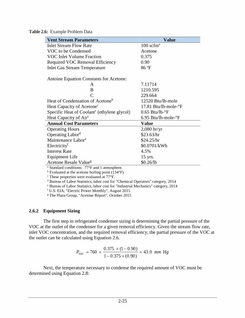
2.6.1 Required Information for Design

The first step in the design procedure is to specify the gas stream to be processed. Gas

stream parameters to be used in this example problem are listed in Table 2.6. The values for the

Antoine equation constants, heat of condensation, and heat capacity of acetone are obtained from

Appendix A. Specific heat of the coolant is obtained from Perry’s Chemical Engineers’

Handbook (Green, 2008).

2-25

Table 2.6: Example Problem Data

Vent Stream Parameters Value

Inlet Stream Flow Rate 100 scfma

VOC to be Condensed Acetone

VOC Inlet Volume Fraction 0.375

Required VOC Removal Efficiency 0.90

Inlet Gas Stream Temperature 86 ºF

Antoine Equation Constants for Acetone:

A 7.11714

B 1210.595

C 229.664

Heat of Condensation of Acetoneb 12520 Btu/lb-mole

Heat Capacity of Acetonec 17.81 Btu/lb-mole-°F

Specific Heat of Coolantc (ethylene glycol) 0.65 Btu/lb-°F

Heat Capacity of Airc 6.95 Btu/lb-mole-°F

Annual Cost Parameters Value

Operating Hours 2,080 hr/yr

Operating Labord $23.63/hr

Maintenance Labore $24.25/hr

Electricityf $0.0701/kWh

Interest Rate 4.5%

Equipment Life 15 yrs.

Acetone Resale Valueg $0.26/lb a Standard conditions: 77°F and 1 atmosphere. b Evaluated at the acetone boiling point (134°F). c These properties were evaluated at 77°F. d Bureau of Labor Statistics, labor cost for "Chemical Operators" category, 2014 e Bureau of Labor Statistics, labor cost for "Industrial Mechanics" category, 2014 f U.S. EIA, "Electric Power Monthly", August 2015 g The Plaza Group, "Acetone Report", October 2015

2.6.2 Equipment Sizing

The first step in refrigerated condenser sizing is determining the partial pressure of the

VOC at the outlet of the condenser for a given removal efficiency. Given the stream flow rate,

inlet VOC concentration, and the required removal efficiency, the partial pressure of the VOC at

the outlet can be calculated using Equation 2.6.

HgmmPVOC

0.43)90.0(375.01

)90.01(375.0760

Next, the temperature necessary to condense the required amount of VOC must be

determined using Equation 2.8:

2-26

FTcon

16328.1664.229

)43(log11714.7

595.1210

10

The next step is to estimate the VOC condenser heat load. Calculate: (1) the VOC flow

rate for the inlet/outlet emission streams, (2) the flow rate of the condensed VOC, and (3) the

condenser heat balance. The flow rate of VOC in the inlet stream is calculated from

Equation 2.9.

hr

moleslbM

inVOC

740.560375.0

392

100,

The flow rate of VOC in the outlet stream is calculated using Equation 2.2 as follows:

hr

moleslbM

outVOC

5740.0)90.01(740.5

,Finally, the flow rate of condensed VOC

is calculated with Equation 2.10:

hr

moleslbM

recoveredVOC

166.5574.0740.5

,

Next, the condenser heat balance is conducted. As indicated in Table 2.6, the acetone heat

of condensation is evaluated at its boiling point, 134°F. However, it is assumed (for simplicity)

that all of the acetone condenses at the condensation temperature, Tcon = 16°F. To estimate the

heat of condensation at 16°F, use the Watson equation (Equation 2.14) with the following inputs:

Tc = 915 °R (from Appendix A)

T1 = 134 + 460 = 594 °R

T2 = 16 + 460 = 476 °R

Upon substitution, we obtain:

molelb

Btu

FatHVOC

090,14

915

5941

915

4761

520,1216

38.0

As Table 2.6 shows, the heat capacities of acetone and air and the specific heat of the

coolant were all evaluated at 77°F. This temperature is fairly close to the condenser mean

operating temperature, i.e., (86 + 16)/2 = 51°F. Consequently, using the 77°F values would not

add significant additional error to the heat load calculation.

2-27

The change in enthalpy of the condensed VOC is calculated using Equation 2.12:

hr

BtuH

con230,79168681.17090,14166.5

The enthalpy change associated with the uncondensed VOC is calculated from

Equation 2.16:

hr

BtuH

uncon6.715)1686()81.17()574.0(

Finally, the enthalpy change of the noncondensible air is estimated from Equation 2.17:

hr

BtuH

noncon654,4)1686(95.6740.560

392

100

The condenser heat load is then calculated by substituting ∆Hcon, ∆Huncon, and ∆Hnoncon in

Equation 2.11:

hr

BtuH

load600,84654,46.715230,79

The next step is estimation of the VOC condenser size. The logarithmic mean

temperature difference is calculated using Equation 2.19. In this calculation, from Equations 2.20

and 2.21, respectively:

Tcool,in = 16 - 15 = 1°F

Tcool,out = 1 + 25 = 26°F

and:

FT

lm

5.32

116

2686ln

1162686

The condenser surface area can then be calculated using Equation 2.18.

22.130

)5.32(20

600,84ftA

con

In this equation, a conservative value of 20 Btu/hr-ft2-°F is used as the overall heat

transfer coefficient.

2-28

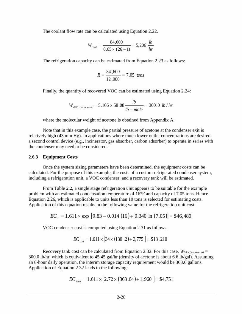
The coolant flow rate can be calculated using Equation 2.22.

hr

lbW

cool206,5

)126(65.0

600,84

The refrigeration capacity can be estimated from Equation 2.23 as follows:

tonsR 05.7000,12

600,84

Finally, the quantity of recovered VOC can be estimated using Equation 2.24:

hrlbmolelb

lbW

eredreVOC/0.30008.58166.5

cov,

where the molecular weight of acetone is obtained from Appendix A.

Note that in this example case, the partial pressure of acetone at the condenser exit is

relatively high (43 mm Hg). In applications where much lower outlet concentrations are desired,

a second control device (e.g., incinerator, gas absorber, carbon adsorber) to operate in series with

the condenser may need to be considered.

2.6.3 Equipment Costs

Once the system sizing parameters have been determined, the equipment costs can be

calculated. For the purpose of this example, the costs of a custom refrigerated condenser system,

including a refrigeration unit, a VOC condenser, and a recovery tank will be estimated.

From Table 2.2, a single stage refrigeration unit appears to be suitable for the example

problem with an estimated condensation temperature of 16°F and capacity of 7.05 tons. Hence

Equation 2.26, which is applicable to units less than 10 tons is selected for estimating costs.

Application of this equation results in the following value for the refrigeration unit cost:

480,46$05.7ln340.016014.083.9exp611.1 r

EC

VOC condenser cost is computed using Equation 2.31 as follows:

210,13$775,32.13034611.1 con

EC

Recovery tank cost can be calculated from Equation 2.32. For this case, WVOC,recovered =

300.0 lb/hr, which is equivalent to 45.45 gal/hr (density of acetone is about 6.6 lb/gal). Assuming

an 8-hour daily operation, the interim storage capacity requirement would be 363.6 gallons.

Application of Equation 2.32 leads to the following:

751,4$960,164.36372.2611.1tank

EC

2-29

Assuming there are no additional costs due to precooler or other auxiliary equipment, the

total equipment cost is calculated from Equation 2.33:

64,440$=0+0+4,751+13,210+46,480=c

EC

The purchased equipment cost including instrumentation, controls, taxes, and freight is

estimated using Equation 2.34:

040,76$440,6418.1 c

PEC

Using the default contingency factor of 0.10, the contingency cost (C) is estimated as

follows:

000,13$040,7671.110.0 C

The total capital investment is calculated using Equation 2.37:

000,145$000,13040,7671.1 TCI

2.6.4 Total Annual Cost

Table 2.7 summarizes the estimated annual costs for the example problem. The cost

calculations are shown in the table.

Direct annual costs for refrigerated systems include labor, materials, and utilities. Labor

costs are based on 8-hr/day, 5-day/week operation. Supervisory labor is computed at 15 percent

of operating labor, and operating and maintenance labor are each based on 1/2 hr per 8-hr shift.

The electricity cost is based on a requirement of 2.2 kW/ton (see Table 2.5), because the

condensation temperature (16°F) is close to the 20°F temperature given for this value.

Indirect annual costs include overhead, capital recovery, administrative charges, property

tax, and insurance.

Total annual cost is estimated using Equation 2.41. For this example, application of

refrigerated condensation as a control measure results in an annual savings of $122,000. As

Table 2.7 shows, the acetone recovery credit is approximately four times the direct and indirect

costs combined. Clearly, this credit has more influence on the total annual cost than any other

component. Although the credit depends on three parameters―the acetone recovery rate, the

annual operating hours, and the acetone salvage value ($0.26/lb) (Dunn, 2015) ―the last

parameter is often the most difficult to estimate. This is mainly because the salvage value varies

according to the facility location and its local market as well as the current state of the broader

chemical market.

2-30

Table 2.7: Annual Cost for Refrigerated Condenser System Example Problem

Cost Item Calculations Cost

Direct Annual Costs, DAC

Operating Labor

Operator 0.5 ℎ

𝑠ℎ𝑖𝑓𝑡×

𝑠ℎ𝑖𝑓𝑡

8 ℎ×

2,080 ℎ

𝑦𝑟×

$23.63

ℎ $3,072

Supervisor 0.15 ×$3,070 460.80

—

Maintenance

Maintenance Labor 0.5 ℎ

𝑠ℎ𝑖𝑓𝑡×

𝑠ℎ𝑖𝑓𝑡

8 ℎ×

2,080 ℎ

𝑦𝑟×

$24.25

ℎ

3,153

Materials 100% maintenance labor 3,153

Utilities

Electricity 7.050 𝑡𝑜𝑛𝑠

0.85×

2.2 𝑘𝑊

𝑡𝑜𝑛×

2,080 ℎ

𝑦𝑟

×$0.0701

𝑘𝑊ℎ

2,661

Total DAC $12,500

Indirect Annual Costs, IAC

Overhead 0.6 × (3,072 + 460.8 + 3,153 + 3,153) 5,903

Administrative charges 0.02 ($145,000) 2,900

Property tax 0.01 ($145,000) 1,450

Insurance 0.01 ($145,000) 1,450

Capital recoverya 0.0915 × $145,000 13,270

Total IAC $24,970

Recovery Credits, RC

Recovered Acetone (rounded) 300 𝑙𝑏

ℎ×

2,080 ℎ

𝑦𝑒×

$0.26

𝑙𝑏

($162,200)

Total Annual Cost (rounded) $12,500 + $27,620 – ($162,200) ($122,000)

(Savings) a For CRC, assumed interest rate is 4.25% and the equipment life is 15 years, for a capital recovery factor of 0.0915.

2-31

2.7 Example Problem 2

In this example problem, the alternate design procedure described in Section 2.3.8 is

illustrated. The temperature of condensation is given, and the resultant removal efficiency is

calculated. The example stream inlet parameters are identical to Example Problem 1 with the

exception that removal efficiency is not specified and the required temperature of condensation

is assumed to be 16 °F.

2.7.1 Required Information for Design

The first step is to calculate the partial pressure of the VOC at the specified temperature

(16 °F) using Equation 2.7 to solve for PVOC:

CT

BAP

con

VOC

10

log

Remember to convert Tcon to degrees Centigrade, i.e., 16 °F = -8.9 °C.

Substituting the values for the Antoine equation constants for acetone as listed in

Table 2.6:

664.2299.8

595.121011714.7log

10

VOC

P

HgmmPVOC

0.43

Using Equation 2.25, the removal efficiency is:

90.00.43760375.0

0.43375.0760

The remainder of the calculations in this problem are identical to those in Example

Problem 1.

2.8 Acknowledgements

The authors gratefully acknowledge the following companies for contributing data to this

chapter:

Edwards Engineering (Pompton Plains, NJ)

Piedmont Engineering (Charlotte, NC)

Universal Industrial Refrigeration (Gonzales, LA)

ITT Standard (Atlanta, GA)

XChanger (Hopkins, MN)

Buffalo Tank Co. (Jacksonville, FL)

2-32

References

Bureau of Labor Statistics, "Chemical Equipment Operators and Tenders", Occupational

Employment and Wages, May 2014. Web. Accessed 27 October 2015.

<http://www.bls.gov/oes/current/oes519011.htm>

Bureau of Labor Statistics, "Industrial Machinery Mechanics", Occupational Employment

and Wages, May 2014. Web. Accessed 27 October 2015.

<http://www.bls.gov/oes/current/oes499041.htm>

Cooke, Avery. Letter and attachment from Liquid Handling Equipment, Inc., to Rich Pelt of

Radian Corporation. 20 September 1990.

Dean, John A., ed. Lange's Handbook of Chemistry. 14th ed. New York: McGraw-Hill, 1992.

Erikson, D.G. U.S. Environmental Protection Agency. "Control Device Evaluation

Condensation." Organic Chemical Manufacturing Volume 5: Adsorption,

Condensation, and Absorption Devices. EPA-450/3-80-027. Research Triangle Park:

U.S. Environmental Protection Agency, Office of Air Quality Planning and

Standards, December 1980.

Green, Don W., ed. Perry's Chemical Engineers' Handbook. 8th ed. New York: McGraw-

Hill, 2008.

Hansek, Bob. Letter and attachment from ITT Corporation to Wiley Barbour of Radian

Corporation. 10 October 1990.

Kern, D. Q. Process Heat Transfer. New York: McGraw-Hill, 1950.

Lozowski, Dorothy, et al., eds. "Economic Indicators." Chemical Engineering October 2015:

104.

McCabe, W. L., and J. C. Smith. Unit Operations of Chemical Engineering. 3rd ed. New

York: McGraw-Hill, 1976.

Pohanish, Richard P., and Stanley A. Greene. Hazardous Materials Handbook. New York:

Van Nostrand Reinhold, 1996

Price, Brian C. "Know the Range and Limitations of Screw Compressors." Chemical

Engineering Progress 87.2. 1991: 50-56.

Poling, B.E., J.M. Prausnitz, and J.P. O’Connell. Properties of Gases & Liquids. 5th ed. New

York: McGraw-Hill, 2001

Sisk, Robert V., Jr. Letter and attachment from Piedmont Engineering Corp. to Wiley

Barbour of Radian Corporation. 28 January 1991.

2-33

Smith, J. M., M. C. VanNess, and M. M. Abbott. Introduction to Chemical Engineering

Thermodynamics. 7th ed. New York: McGraw-Hill, 2005.

Speight, James G., ed. Lange's Handbook of Chemistry. 16th ed. New York: McGraw-Hill,

2005.

The Plaza Group, "Newsletters: Acetone Report", October 2015. Web. 27 October 2015.

<http://www.theplazagrp.com/newsletters.asp?id=2>

U.S. Environmental Protection Agency, "Technical Bulletin: Refrigerated Condensers for

Control of Organic Air Emissions", EPA-456/R-01-004. Research Triangle Park: U.S.

Environmental Protection Agency, Clean Air Technology Center, December 2001.

U.S. Energy Information Administration. "Electric Power Monthly: Data for August 2015."

Web. Accessed October 2015.

<http://www.eia.gov/electricity/monthly/epm_table_grapher.cfm?t=epmt_5_3>

U.S. Environmental Protection Agency. "Significant New Alternative Policy (SNAP)

Program website." Accessed October 2015. <http://www2.epa.gov/snap>

Vatavuk, William M. "Updating the CE Plant Cost Index." Chemical Engineering January

2002: 63.

Vatavuk, W. M., and R. B. Neveril. "Estimating Costs for Air Pollution Control Systems,

Part II: Factors for Estimating Capital and Operating Costs." Chemical Engineering.

November 1980: 157-162.

Vatavuk, W. M., and R. B. Neveril. "Estimating Costs of Air Pollution Control Systems: Part

XVI: Costs of Refrigeration Systems." Chemical Engineering. 16 May 1983: 95-98.

Waldrop, Richard. Letter from Edwards Engineering Corp. to William Vatavuk. 29 August

1988.

Waldrop, R., and V. Sardo. Letter and attachment from Edwards Engineering Corp. to Wiley

Barbour of Radian Corporation. 1 October 1990.

2-34

Appendix A

Properties of Selected Compounds

2-35

Table A-1: Physical Properties for Selected Compounds

a Reprinted with permission from the 16th edition of Lange's Handbook of Chemistry, Table 2.55 (Speight, 2005). b Reprinted with permission from the 16th edition of Lange's Handbook of Chemistry, Table 2.54 (Speight, 2005).

(Measured at boiling point). c Reprinted with permission from the 16th edition of Lange's Handbook of Chemistry, Table 2.53 (Speight, 2005).

(Measured at 77 °F). d These values are taken from the 14th edition of Lange's Handbook of Chemistry (Dean, 1992).

Compound

Critical Temp.a

(°R)

Boiling Point (°F)

Molecular Weight

(lb/lb-mole)

Heat of Condensationb

(Btu/lb-mole) Heat Capacityc (Btu/lb-mole-°F) State

Acetone 915 134 58.08 12,520 30.19 Liquid

17.81 Gas

Acetylene 555 -119 26.02 7,310 10.54 Gas

Acrylonitrile 965 171 53.06 14,030 15.25 Gas

Aniline 1258 364 93.13 18,240 45.87 Liquid

25.79 Gas

Benzene 1012 176 78.11 13,210 32.51 Liquid

Benzonitrile 1259 375 d 103.12 19,750 26.08 Gas

Butane 765 31 58.12 9,640 23.31 Gas

Chloroethane 829 54 64.52 10,630 14.96 Gas

Chloroform 966 143 119.39 12,560 15.71 Gas

Chloromethane 749 -12 50.49 9,210 9.75 Gas

Cyclobutane 828 55 56.10 10,410 17.26 Gas

Cyclohexane 996 177 84.16 12,910 37.03 Liquid

25.41 Gas

Cyclopentane 921 121 70.13 11,750 30.81 Liquid

19.84 Gas

Cyclopropane 716 -27 42.08 8,650 13.29 Gas

Diethyl ether 840 94 74.12 11,400 41.26 Liquid

28.57 Gas

Dimethylamine 787 44 45.09 11,360 16.90 Gas

Ethylbenzene 1111 277 106.17 15,320 30.69 d Gas

Ethylene oxide 844 51 44.05 10,970 11.45 Gas

Heptane 972 209 100.12 13,680 53.76 Liquid

39.68 Gas

Hexane 914 156 86.18 12,440 46.76 Liquid

34.21 Gas

Methanol 923 148 32.04 15,150 19.41 Liquid

10.54 Gas

Octane 1024 258 114.23 14,800 45.16 Gas

Pentane 845 d 97 72.15 11,100 28.73 Gas

Toluene 1065 231 92.14 14,290 37.53 Liquid

24.76 Gas

o - Xylene 1135 292 106.17 15,880 44.49 Liquid

31.86 Gas

m - Xylene 1111 282 106.17 15,360 43.82 Liquid

30.50 Gas

p - Xylene 1109 281 106.17 15.360 30.33 Gas

2-36

Table A-2: Antoine Equation Constants for Selected Compoundsa

Compound

Antoine Equation Constants Valid Temperature

Range (°F) A B C

Acetone 7.11714 1210.595 229.664 Liquid

Acetylene 9.1402 1232.6 280.9 -202 to -117

7.0999 711.0 253.4 -116 to -98

Acrylonitrile 7.03855 1232.53 222.47 -4 to 284

Aniline 7.32010 1731.515 206.049 216 to 365

Benzene 9.1064 1885.9 244.2 10 to 37

6.90565 1211.033 220.790 46 to 217

Benzonitrile 6.74631 1436.72 181.0 Liquid

n-Butane 6.80898 935.86 238.73 -107 to 66

Chloroethane 6.98647 1030.01 238.61 -69 to 54

Chloroethylene 6.89117 905.01 239.48 -85 to 9

Chloroform 6.4934 929.44 196.03 -31 to 142

Chloromethane 7.09349 948.58 249.34 -103 to 23

Cyanic acid 7.56859 1251.86 243.79 -105 to 21

Cyclobutane 6.91631 1054.54 241.37 -76 to 54

Cyclohexane 6.84130 1201.53 222.65 68 to 178

Cyclopentane 6.88676 1124.162 231.36 -40 to 162

Cyclopropane 6.88788 856.01 246.50 -130 to -26

Diethyl ether 6.92032 1064.07 228.80 -78 to 68

Diethylamine 5.8016 583.30 144.1 88 to 142

Dimethylamine 7.08212 960.242 221.67 -98 to 44

1,4-Dioxane 7.43158 1554.68 240.34 68 to 221

Ethylbenzene 6.95719 1424.255 213.21 79 to 327

Ethylene oxide 7.12843 1054.54 237.76 -56 to 54

Heptane 6.89677 1264.90 216.54 28 to 255

Hexane 6.87601 1171.17 224.41 -13 to 198

Methanol 7.89750 1474.08 229.13 7 to 149

7.97328 1515.14 232.85 147 to 230

Octane 6.91868 1351.99 209.15 66 to 306

Pentane 6.85296 1064.84 233.01 -58 to 136

Toluene 6.95464 1344.800 219.48 43 to 279

Vinyl acetate 7.2101 1296.13 226.66 72 to 162

2-37

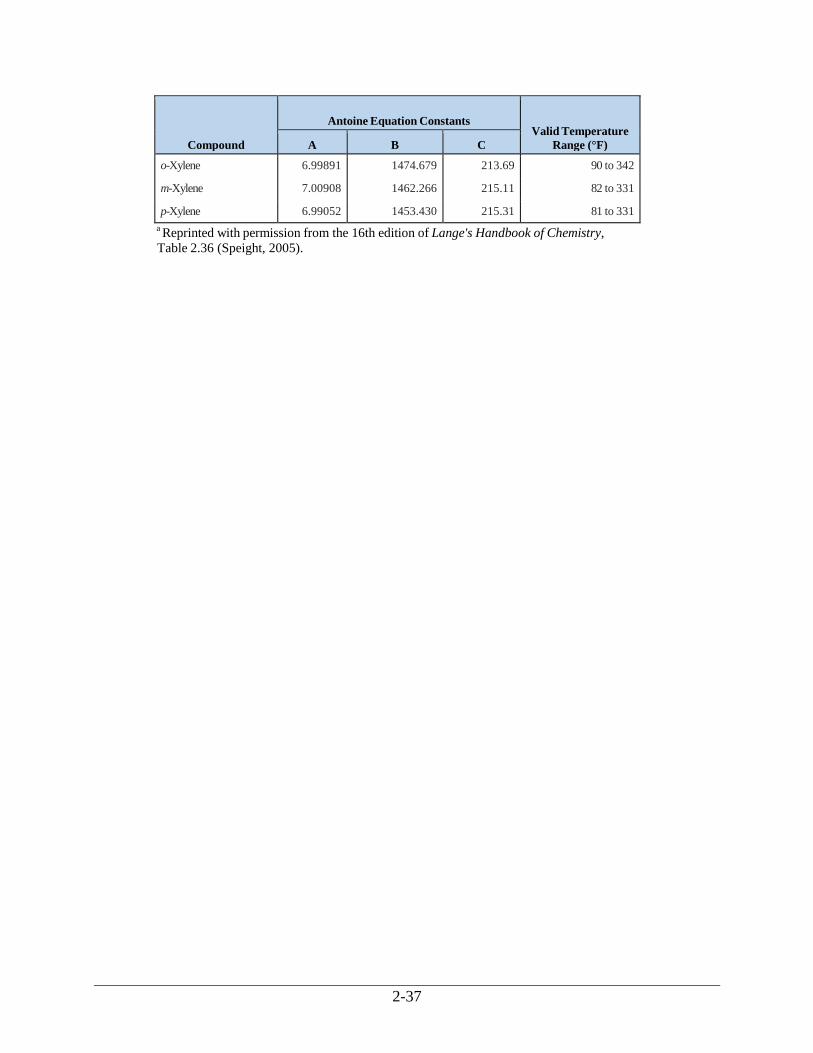
Compound

Antoine Equation Constants Valid Temperature

Range (°F) A B C

o-Xylene 6.99891 1474.679 213.69 90 to 342

m-Xylene 7.00908 1462.266 215.11 82 to 331

p-Xylene 6.99052 1453.430 215.31 81 to 331

a Reprinted with permission from the 16th edition of Lange's Handbook of Chemistry,

Table 2.36 (Speight, 2005).

2-38

Appendix B

Documentation for Gasoline Vapor

Recovery System Cost Data

2-39

As mentioned in Section 2.4.3, vendor cost data were obtained that related the equipment

cost ($) of packaged gasoline vapor recovery systems to the process flow capacity (gal/ min).

These data needed to be transformed, in order to develop Equation 2.35, which relates equipment

cost ($) to system refrigeration capacity (R, tons), as follows:

212,000 +4,910R = ECp

To make this transformation, we needed to develop an expression relating flow capacity

to refrigeration capacity. The first step was to determine the inlet partial pressure (PVOC,in) of the

VOC—gasoline, in this case. As was done in Section 3.1, we assumed that the VOC vapor was

saturated and, thus, in equilibrium with the VOC liquid. This, in turn, meant that we could equate

the partial pressure to the vapor pressure. The “model” gasoline had a Reid vapor pressure of 10

and a molecular weight of 66 lb/lb-mole, as shown in Section 7.1 of Compilation of Air Pollutant

Emission Factors (EPA publication AP-42, Fifth Edition, November 2006). For this gasoline, the

following Antoine equation constants were used:

A = 6.2236

B = 944.81

C = 233

These constants were obtained by extrapolating available vapor pressure vs. temperature

data for gasoline found in Section 7.1 of AP-42. Upon substituting these constants and an

assumed inlet temperature of 77 °F (25 °C) into the Antoine equation and solving for the inlet

partial pressure (PVOC,in). We obtain:

CT

BAP

in

inVOC

,

log

23325

81.9442236.6

HgmmPinVOC

365,

If the system operates at atmospheric pressure (760 mm Hg), this partial pressure would

correspond to a VOC volume fraction in the inlet stream of:

480.0760

365,

mm

mmY

inVOC

The outlet partial pressure (Pvoc,out) and volume fraction are calculated in a similar way.

The condensation (outlet) temperature used in these calculations is -80°F (-62°C), which is the

typical operating temperature for the gasoline vapor recovery units for which the vendor supplied

costs.

HgmmP

P

outVOC

outVOC

01.5

23362

81.9442236.6log

,

,

2-40

This corresponds to a volume fraction in the outlet stream (yVOC,out) of:

0066.0760

01.5,

mm

mmy

outVOC

Substitution of PVOC,out and yVOC,in into Equation 2.25 yields the condenser removal

efficiency:

993.0

01.5760480.0

01.5480.0760

The next step is determining the inlet and outlet VOC hourly molar flow rates (MVOC,in

and MVOC,out, respectively). As Equation 2.9 shows, MVOC,in is a function of yVOC,in and the total

inlet volumetric flow rate, Qin, (scfm).

Now, because the gasoline vapor flow rates are typically expressed in gallons/minute, we

have to convert them to scfm. This is done as follows:

scfmQgal

ftgalQQ

ggin134.0

48.7

1

min

3

Substituting these variables into Equation 2.9, we obtain:

hr

molelbQ

QM

g

g

inVOC

00984.060480.0

392

134.0,

We obtain MVOC,out from Equation 2.2:

hr

moleslbQQM

ggoutVOC

5

,1089.6993.0100984.0

And according to Equation 2.10, the amount of gasoline vapor condensed (MVOC,recovered)

is the difference between MVOC,in and MVOC,out:

hr

moleslbQM

geredreVOC00977.0

cov,

The final step is to calculate the condenser heat load. This load is a function of the inlet,

outlet, and condensate molar flow rates, the inlet and condensation temperatures, the heat

capacities of the VOC and air, and the VOC heat of condensation. The VOC heat capacity used

are based on pentane and butane chemical properties, the largest components of gasoline, and

were obtained from Lange’s Handbook of Chemistry (16th edition). The heat of condensation

data were obtained for gasoline from CHRIS Hazardous Chemical Data (U.S. Coast Guard, U.S.

Department of Transportation, June 1999).

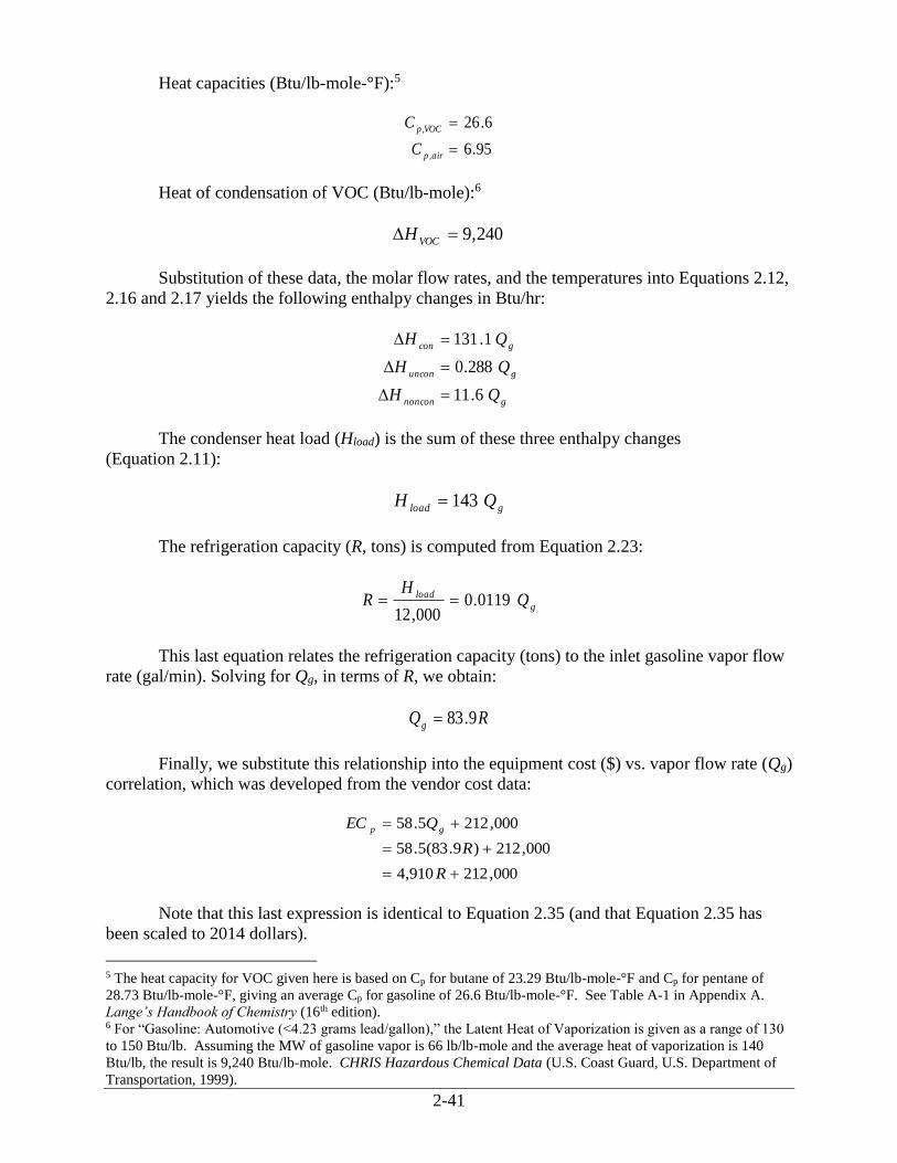
2-41

Heat capacities (Btu/lb-mole-°F):5

95.6

6.26

,

,

airp

VOCp

C

C

Heat of condensation of VOC (Btu/lb-mole):6

240,9VOC

H

Substitution of these data, the molar flow rates, and the temperatures into Equations 2.12,

2.16 and 2.17 yields the following enthalpy changes in Btu/hr:

gnoncon

guncon

gcon

QH

QH

QH

6.11

288.0

1.131

The condenser heat load (Hload) is the sum of these three enthalpy changes

(Equation 2.11):

gloadQH 143

The refrigeration capacity (R, tons) is computed from Equation 2.23:

g

load QH

R 0119.0000,12

This last equation relates the refrigeration capacity (tons) to the inlet gasoline vapor flow

rate (gal/min). Solving for Qg, in terms of R, we obtain:

RQg

9.83

Finally, we substitute this relationship into the equipment cost ($) vs. vapor flow rate (Qg)

correlation, which was developed from the vendor cost data:

000,212910,4

000,212)9.83(5.58

000,2125.58

R

R

QECgp

Note that this last expression is identical to Equation 2.35 (and that Equation 2.35 has

been scaled to 2014 dollars).

5 The heat capacity for VOC given here is based on Cp for butane of 23.29 Btu/lb-mole-°F and Cp for pentane of

28.73 Btu/lb-mole-°F, giving an average Cp for gasoline of 26.6 Btu/lb-mole-°F. See Table A-1 in Appendix A.

Lange’s Handbook of Chemistry (16th edition). 6 For “Gasoline: Automotive (<4.23 grams lead/gallon),” the Latent Heat of Vaporization is given as a range of 130

to 150 Btu/lb. Assuming the MW of gasoline vapor is 66 lb/lb-mole and the average heat of vaporization is 140

Btu/lb, the result is 9,240 Btu/lb-mole. CHRIS Hazardous Chemical Data (U.S. Coast Guard, U.S. Department of

Transportation, 1999).