Chapter 2: The Heckscher Ohlin Samuelson model

Globalization- Econ 102

1 IntroductionWe saw in the Ricardo model that international trade can be mutually beneficial to

the nations engaged in it. Yet through history, governments have protected sectors of theeconomy from import competition. For example, despite its commitment in principle tofree trade, the United States limits imports of textiles, sugar and other commodities. Iftrade is such a good thing for the economy, why is there opposition to its effects? Tounderstand the politics of trade, it is necessary to look at the effects of trade, not just ona country as a whole but on the distribution of income within that country.

The Ricardian model of international trade illustrates the potential benefits from trade.In that model trade leads to international specialization, with each country shifting itslabor force from industries in which that labor is relatively inefficient to industries inwhich it is relatively more efficient. Because labor is the only factor of production in themodel, and it is assumed to be able to move freely from one industry to another, there isno possibility that individuals will be hurt by trade. The Ricardian model thus suggestsnot only that all countries gain from trade, but that every individuals is made better ofas a result of international trade, because trade does not affect the distribution of income.In the real world, however, trade has substantial effects on the income distribution withineach trading nation, so that in practice the benefits of trade are often distributed veryunevenly.

There are two main reasons why international trade has strong effects on the distri-bution of income. First, resources cannot move immediately or without cost from oneindustry to another. Second, industries differ in the factor of production they demand: Ashift in the mix of goods that a country produces will ordinarily reduce the demand forsome factors of production, while raising the demand for others.

The Heckscher-Ohlin model fills this gap by considering two production factors ratherthan only one as in the Ricardian model. The Heckscher-Ohlin (HO hereafter) model wasfirst conceived by two Swedish economists, Eli Heckscher and Bertil Ohlin. Rudimentaryconcepts were further developed and added later by Paul Samuelson and Ronald Jonesamong others. Heckscher was a Swedish economist. He is probably best known for hisbook "Mercantilist." Although his major interest was in studying economic history, he alsodeveloped the essentials of the factor endowment theory of international trade. Heckscher’sstudent, Bertil Ohlin developed and elaborated the factor endowment theory. He was notonly a professor of economics at Stockholm, but also a major political figure in Sweden.The Heckscher-Ohlin model is often associated with a third economist: Paul Samuelsonthat increased the prediction of the model.

1

There are four major components of the HO model: (i) Factor Price EqualizationTheorem, (ii) Stolper-Samuelson Theorem, (iii) Rybczynski Theorem, and (iv) Heckscher-Ohlin Trade Theorem.

2 OverviewIf labor were the only factor of production, comparative advantage could arise only be-

cause of international differences in labor productivity. In the real world, however, whiletrade is partly explained by differences in labor productivity, it also reflects differences incountry resources. To explain the role of resource differences in trade, this chapter onlyexamines a model in which resource differences are the only source of trade. This modelshows that comparative advantage is influenced by the interaction between nations’ re-sources (the relative abundance of factors of production) and the technology of production(which influences the relative intensity with which different factors of production are usedin the production of different goods).

To develop the HOS model we begin by describing an economy that does not trade,then ask what happens when two such economies trade with each other.

The HOS model is a prolongation of the Ricardian model with two resources, twogoods and two countries. The originality of the HOS model is to consider two productionfactors rather than only one as in the Ricardian model that was labor. There are fourmain assumptions in this model:

• Factors are mobile across sectors but immobile across countries

• There is no transportation costs

• Pure and perfect competition exists (no firms are price makers) and there is fullemployment

• The production function is with constant return to scale and decreasing marginalproductivity

3 The modelThe simplest way of understanding the HOS model is to consider two economies that

can produce two goods. For the rest of this chapter we will consider that the two economiesare Home (no asterisk) and the rest of the world (ROW, with asterisk). The two economiescan produce two goods: cotton and wheat and the production function takes the Cobb-Douglas form, defined as follows.

W = H12L

12

C = H13L

23

Production of these goods requires two inputs that are in limited supply: high-skilledlabor and low-skilled labor. As in the previous chapter, let us defined the following ex-pression:

αHW → is the hours of skilled labor used to produce one pound of wheat

2

αHC → is the hours of skilled labor used to produce one pound of cotton

αLW → is the hours of unskilled labor used to produce one pound of wheat

αHW → is the hours of unskilled labor used to produce one pound of wheat

L̄→ is the economy’s supply of labor in the home country

L̄∗ → is the economy’s supply of labor in the foreign country

The technology used to produce the two commodities are different. Let’s assume thatone unit of wheat requires one unit of low-skilled workers and two units of high-skilledworkers and one unit of cotton requires two units of low-skilled workers and one unitof high-skilled workers. The fact that technologies are different between sectors meansthat one factor is intensive in one factor of production and the other is intensive in theother factor of production. Sectors differ in the extent to which they use the factors ofproduction. Each sector’s demand for the factors depends on the sector’s factor intensity.From our previous example Cotton is low-skilled workers intensive and Wheat is high-skilled workers intensive. In other words, sector W (that stands for wheat) intensely usesthe H factor of production which means that Hw

Lwis relatively high compared to the cotton

sector.

The cost of producing a good depends on factor prices: if the cost of high-skilled laboris higher than the cost of low-skilled labor then other things equal the price of any goodwhose production involves high-skilled labor input will also have to be higher. Here, weassume that high-skilled workers in each country earn the wage wH , and low-skilled workersearn the wage wL. Workers are mobile across sectors within a country, but every factoris trapped within its country’s borders. In other words, workers can move from sectorto sector within each country but not move from country to country. In equilibrium,high-skilled workers in any sector all earn the same wage wH as the high-skilled workersemployed in another sector. Low-skilled workers also earn the same wage wL no matterin which sector they are employed. If any sector were to pay a higher wage, the workerwould switch employment. In equilibrium, when no worker wants to switch jobs, each skillgroup of workers must therefore earn the same wage.

From the two Cobb-Douglas functions we can see that the production of Cotton isrelatively low-skilled intensive while the production of Wheat is relatively high-skilledintensive. The price of Wheat will be relatively high compared to Cotton.

Every country has a supply of human resources, which are referred to as an endowment.The allocation of resources in each country are different from one country to another.These resources are factors of production used to generate output. We say a country isrelatively abundant in a factor if the country is relatively well endowed with that factor.Let us write H the economy’s supply of high-skilled labor and L the economy’s supply oflow-skilled labor in the home country. H∗ is the economy’s supply of high-skilled workersand L∗ is the economy’s supply of low-skilled workers in the Foreign country. We assumethat Home (the United-States) is high-skilled labor abundant and Foreign (the Rest of theWorld (ROW)) is low-skilled labor abundant. This assumption implies that H

L > H∗

L∗ .

We now have all the ingredients in place that make up the basic Heckscher-Ohlin modeland we can start to derive the main insights. There are several important predictions of thismodel, and theorems summarize those predictions. Each theorem is a result that inevitablyfollows from the fundamentals of the model (as listed here). First, the Heckscher-Ohlintheorem (about the Heckscher-Ohlin model) states how factor abundance and the sectors’factor intensities predict trade flows. Second, you will see how changing trade flows and

3

product prices translate back into a country’s income distribution because they affect theproduction factors’ earnings in the Heckscher-Ohlin model; this is the Stolper-Samuelsontheorem. Third, you will get to know how migration relates to trade and factor earningsin the model; that is what the Rybczynski theorem covers. In the next chapter, you willfinally see under what conditions the Heckscher-Ohlin model predicts that factor earningsaround the world will become more similar to each other (the Factor Price Equalizationtheorem). One model, four theorems.

3.1 Curved Production Possibilities and the Heckscher-Ohlin theorem

In Ricardian trade theory, the production possibility frontier (PPF) for two sectorsis a straight line. Among other consequences, Ricardian trade therefore results in com-plete specialization: Every sector produces in only one location under free trade. Inclassic trade theory with more than one factor of production, in contrast, the PPF is bellyshaped. Among other implications, the curved PPF results in incomplete specialization:A country’s export sector produces relatively more output than the world average, andthe country’s import-competing sector produces relatively less than the world average,but each sector typically produces in both locations under free trade. To understand whyproduction possibilities are curved when there are constant returns to scale but more thantwo factors of production, let us draw the two PPF with our example.

The two PPF of our economies are defined as follows:

A change in a country’s production mix on the PPF means that one sector mustshrink while the other expands. As one sector lays off workers and shrinks, it dismissesrelatively more workers from one skill group than the other sector currently employs.Conversely, as a sector expands, its factor intensity must change because it cannot attractadditional employment given the old skill composition from the shrinking sector. Thismeans the output in the expanding sector must rise less than proportionally. Why? Recallthat constant returns to scale imply that when a sector doubles both factor inputs, thenoutput doubles. When the sector triples both factor inputs, then output triples, and soon. However, when the sector doubles only one factor input and less than doubles theother input, then output less than doubles, and so on. Therefore, if sectors differ in their

4

relative uses of production factors, contracting one sector’s output does not expand theother sector’s output at a constant rate. The expanding sector ends up with a higherproportion of the factor that the sector does not want to use intensively, so production inthe expanding sector increases less than proportionally and the PPF becomes a curve.

In the Ricardo model, because PPF was a straight line each country specializes in onlyone sector, which was not very realistic. Here, because we have a belly shaped curve, wecan get incomplete specialization. A country can still produce both goods even after freetrade. We will see why in the following sections.

Proof that in equilibrium MRT = PwPc

. A way to prove this equality is through themarginal costs. The MRT corresponds to the ratio of marginal costs of the good on thehorizontal axis in terms of the marginal cost of the good on the vertical axis.

Suppose that we want to increase by one unit the quantity of wheat. Recall that we areat full employment, so producing one more unit of wheat implies displacing productionfactors out of the Cotton sector to go to the Wheat sector. The additional cost of thisdisplacement in the Wheat sector can be written as:

dCw = wHdH + wLdL

Because we are in equilibrium and the wage rate in both sector is equal, the cost in theCotton sector goes down by as much.

dCw = −dCC

We saw that MRT is equal to the ratio of the marginal cost. How is defined marginal cost?It corresponds to the cost of the last unit produced. Mathematically this corresponds tothe first order derivative of the cost, defined as follows.

MCw = dCw

dQwand MCc = dCc

dQc

So the ratio of marginal costs can be written

MCw

MCc= dCw

dQw

dQc

dCc

And since we have dCw = −dCc we can write MCwMCc

= −dQc

dQw

We saw in the previous chapter that −dQc

dQwcorresponds to the opportunity cost of wheat

(how many cotton do I need to sacrifice to obtain one more unit of wheat).

Since the marginal cost is equal to the price in equilibrium, we can write the MRT asfollows.

MRT = −dQc

dQw= Pw

Pc

The slope of the PPF corresponds to the rate at which a producer needs to sacrifice

5

one good in order to produce one unit of the other good. This corresponds in economicterms to the marginal rate of transformation (MRT). In equilibrium the MRT is equal tothe relative price of the good on the horizontal axis in terms of the price of the good onthe vertical axis.

If we look at the two PPF, we can see that the US PPF is biased towards the productionof wheat (US produces relatively more wheat than cotton). This result seems intuitivebecause the production of wheat is intensive in skilled labor and US is intensive in skilledlabor. While the PPF of the ROW is biased towards the production of Cotton becauseROW is relatively more intensive in unskilled labor and the production of cotton requiresrelatively more skilled labor.

In order to define the equilibrium relative price under autarky, we need to draw theconsumption ray. We need to specify some type of global consumer preferences. Asconsumers grow richer and richer, it is rational for them to choose combinations of the twoproducts that lie further to the right and up in the graph. We will assume that consumerpreferences are linear which means that the product combinations consumers choose allsit on a ray emanating from the origin of the graph.

The slope of the PPF at the point of intersection between the consumption ray and thePPF gives the equilibrium relative price. We observe that

(PwPc

)ROW

>(

PwPc

)US

, whichmeans that the US has a comparative advantage in the production of wheat because theslope of the PPF is lower in the US than in ROW.

After free trade, the world price will set up in-between these two limits.

(Pw

Pc

)US

<

(Pw

Pc

)F T (freetrade)

<

(Pw

Pc

)ROW

Graphically, the new equilibrium after free trade is obtained when there is a tangencybetween the international trade line (which has a negative slope equals to the relative priceof the good in the horizontal axis in terms of the good in the vertical axis

(PwPc

)F T

) andthe PPF.

6

The red line corresponds to the consumption ray. The two blue lines reflect the slopeof the PPF in equilibrium (when there the consumption ray intersects the PPFs). Recallthat the slope of the PPF in equilibrium corresponds to the relative price of wheat in termsof cotton under autarky for each country. The green line corresponds to the internationaltrade line. The optimal production mix will be obtained when there is a tangency betweenthe PPF and the international trade line. The quantity depicted in the horizontal andvertical axis corresponds to the optimal quantity produced after free trade in the rest of theworld and in the US. The world trade equilibrium results in incomplete specialization.

To summarize, the principle of comparative advantage also predicts the direction oftrade flows and the pattern of specialization. Free markets provide the right price incen-tives to each country’s producers so that they will indeed specialize in the goods in whichthey have the lower opportunity cost of producing.

Once economies are open to free trade, the relative word price of one good in termsof the other is going to lie between the opportunity costs of producing it in the countries.We now study this world price ratio carefully, and give it a name of its own: the termsof trade.

The terms of trade (ToT) are a ratio of product prices on the world market. If thereare only two sectors, then the terms of trade are the price of a country’s exported gooddivided by the price of the country’s imported good on the world market.

ToT = Pexport goodPimport good

We can easily see that the US term of trade is PwPc

and the ROW term of trade is PcPw

.Because the world price after free trade lies between the two opportunity costs we have(

PwPc

)US

<(

PwPc

)F T (freetrade)

<(

PwPc

)ROW

. This implies that the US and the ROW termsof trade increase after free trade. So we know that the US will export wheat and ROWwill export cotton

What quantity of wheat will the US export? and what quantity of cotton will ROWexport? To answer this question we need to find the economy’s new consumption choice.Change in relative price implies that consumer preferences will change. How do we findthe economy’s new consumption choices? Consumers want to place a smaller fraction ofgoods in their consumption baskets when the relative price of this particular good rises.This implies that in the US consumer want to place a lower fraction of wheat in theirbasket because the relative price of wheat rises after free trade. The consumption raytherefore turns up as US households consume a larger share of cotton.

In the EU, consumers want to place a lower fraction of cotton in their consumptionbasket because the relative price of cotton rises after free trade. The consumption raytherefore turns down as EU households consume a larger share of wheat.

The intersection of the new consumption ray with the new terms of tradeline is the new consumption choice after terms-of-trade improvement.

These explanations can be illustrated graphically as follows. For clarity matters, wehave decided to report only the PPF of the US on the following graph.

7

The green line corresponds to the international trade line. The optimal amount ofconsumption is obtained with the intersection between the international trade line andthe new consumption ray line (red dashed line). The optimal production is obtainedwhen there is a tangency between the international trade line (green line) and the PPF.The difference between the quantity produced and consumed in each country will givethe excess demand and supply that will be imported and exported respectively. US willexport wheat and import cotton. There are clear gains from trade compared to the closedeconomy case since the new consumption point is higher than the old consumption point(which was materialized by the intersection between the old consumption ray line (redline) and the PPF).

Now, let us summarize what we just found. In the skilled-workers abundant country,the opportunity cost of producing wheat is lower because that sector uses skilled-labor rel-atively more intensely in production. The skilled-workers abundant country has a compar-ative advantage in the production of wheat because this sector uses skilled-labor relativelyintensively.

This implies that the skill-abundant country will export the good that intensivelyuses the economy’s abundant factor. We just found the Heckscher-Ohlin theorem for twocountries.

If there are two sectors, two countries and two factors that are mobilebetween sectors but not countries, then a country exports the good that in-tensively uses the economy’s abundant factor in production and imports thegood that intensively uses the economy’s scarce factor of production

For example, if the US is relatively abundant in capital compared to its trading partnerthen the US should export capital intensive goods. Leontief, a brilliant economist, reacheda paradoxical conclusion in 1947 though. He found that the US, the most capital abundantcountry in the world by any criterion, exported labor-intensive commodities and importedcapital-intensive commodities. This result has come to be known as the Leontief Paradox.To answer this paradox, Baldwin deleted natural resource sectors and added human capitalto the definition of capital.

8

3.2 The Stolper-Samuelson theorem

With the Heckscher-Ohlin theorem in place, and the predictions for the pattern of tradeknown, Wolfgang Stolper and Paul Samuelson set out to look inside an economy that joinsglobal trade in goods. How does globalization of the world product markets translate backinto employment and earnings inside the economy? Their finding is an important theoremof the HOS model, which has a name of its own: the Stolper Samuelson theorem.

Let us investigate the distributional effects of trade in goods on the factor prices withina country. The factor price is the pay of a factor. Here it corresponds to the wage earnedby skilled and unskilled-workers.

We need to find out where the factors get employed and also to find out the relationbetween the relative price of factor and the relative intensity of factors.

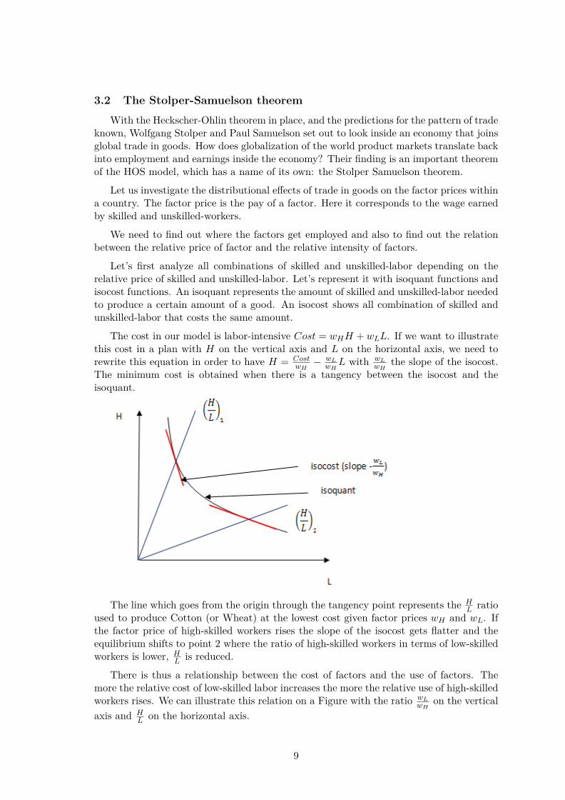
Let’s first analyze all combinations of skilled and unskilled-labor depending on therelative price of skilled and unskilled-labor. Let’s represent it with isoquant functions andisocost functions. An isoquant represents the amount of skilled and unskilled-labor neededto produce a certain amount of a good. An isocost shows all combination of skilled andunskilled-labor that costs the same amount.

The cost in our model is labor-intensive Cost = wHH + wLL. If we want to illustratethis cost in a plan with H on the vertical axis and L on the horizontal axis, we need torewrite this equation in order to have H = Cost

wH− wL

wHL with wL

wHthe slope of the isocost.

The minimum cost is obtained when there is a tangency between the isocost and theisoquant.

The line which goes from the origin through the tangency point represents the HL ratio

used to produce Cotton (or Wheat) at the lowest cost given factor prices wH and wL. Ifthe factor price of high-skilled workers rises the slope of the isocost gets flatter and theequilibrium shifts to point 2 where the ratio of high-skilled workers in terms of low-skilledworkers is lower, H

L is reduced.

There is thus a relationship between the cost of factors and the use of factors. Themore the relative cost of low-skilled labor increases the more the relative use of high-skilledworkers rises. We can illustrate this relation on a Figure with the ratio wL

wHon the vertical

axis and HL on the horizontal axis.

9

The slope in the wheat sector is lower than in the cotton sector because the wheatsector is relatively more intensive in high-skilled labor.

An increase in the relative price of cotton (the good intensive in low-skilled labor)increases the relative price of low-skilled labor and increases the relative intensity of high-skilled workers in both sectors. A decrease in the relative price of cotton (the good intensivein high-skilled labor) reduces the relative price of high-skilled workers in both sectors.

What happens after free trade? We know that free trade leads to a convergence inprice

(PwPc

)US

<(

PwPc

)F T (freetrade)

<(

PwPc

)ROW

.

First, let us analyze what happens in the rest of the world. In the rest of the worldthe relative price of wheat in terms of cotton decreases. Similarly, we can say that therelative price of cotton in terms of wheat increases (

(PcPw

)ROW

). According to what we have

described previously, an increase in(

PcPw

)ROW

increases the relative wage of low-skilledworkers and increases the relative use of high-skilled workers.

Second, let us analyze what happens in the US. In the US, the relative price of wheat interms of cotton increases. Similarly, we can say the the relative price of cotton in terms ofwheat decreases (

(PcPw

)US

). The relative wage of low-skilled workers increases (similarly,the relative wage of high-skilled workers decreases) and the relative use of high-skilledworkers decreases.

This result leads to the Stolper-Samuelson theorem. An increase in the relativeprice of a good will increase the real return to the factor used intensively inthe production of that good, and will decrease the real return to the otherfactor.

Convergence in price of goods, such as illustrated in the last Figure, due to free tradeimplies convergence in relative factor return ( wL

wH) and the relative use of factors in each

sectors.

10

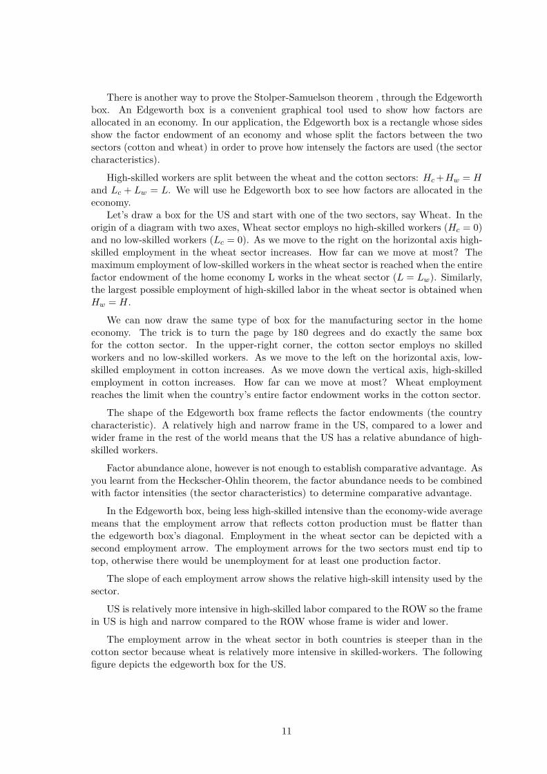
There is another way to prove the Stolper-Samuelson theorem , through the Edgeworthbox. An Edgeworth box is a convenient graphical tool used to show how factors areallocated in an economy. In our application, the Edgeworth box is a rectangle whose sidesshow the factor endowment of an economy and whose split the factors between the twosectors (cotton and wheat) in order to prove how intensely the factors are used (the sectorcharacteristics).

High-skilled workers are split between the wheat and the cotton sectors: Hc +Hw = Hand Lc + Lw = L. We will use he Edgeworth box to see how factors are allocated in theeconomy.

Let’s draw a box for the US and start with one of the two sectors, say Wheat. In theorigin of a diagram with two axes, Wheat sector employs no high-skilled workers (Hc = 0)and no low-skilled workers (Lc = 0). As we move to the right on the horizontal axis high-skilled employment in the wheat sector increases. How far can we move at most? Themaximum employment of low-skilled workers in the wheat sector is reached when the entirefactor endowment of the home economy L works in the wheat sector (L = Lw). Similarly,the largest possible employment of high-skilled labor in the wheat sector is obtained whenHw = H.

We can now draw the same type of box for the manufacturing sector in the homeeconomy. The trick is to turn the page by 180 degrees and do exactly the same boxfor the cotton sector. In the upper-right corner, the cotton sector employs no skilledworkers and no low-skilled workers. As we move to the left on the horizontal axis, low-skilled employment in cotton increases. As we move down the vertical axis, high-skilledemployment in cotton increases. How far can we move at most? Wheat employmentreaches the limit when the country’s entire factor endowment works in the cotton sector.

The shape of the Edgeworth box frame reflects the factor endowments (the countrycharacteristic). A relatively high and narrow frame in the US, compared to a lower andwider frame in the rest of the world means that the US has a relative abundance of high-skilled workers.

Factor abundance alone, however is not enough to establish comparative advantage. Asyou learnt from the Heckscher-Ohlin theorem, the factor abundance needs to be combinedwith factor intensities (the sector characteristics) to determine comparative advantage.

In the Edgeworth box, being less high-skilled intensive than the economy-wide averagemeans that the employment arrow that reflects cotton production must be flatter thanthe edgeworth box’s diagonal. Employment in the wheat sector can be depicted with asecond employment arrow. The employment arrows for the two sectors must end tip totop, otherwise there would be unemployment for at least one production factor.

The slope of each employment arrow shows the relative high-skill intensity used by thesector.

US is relatively more intensive in high-skilled labor compared to the ROW so the framein US is high and narrow compared to the ROW whose frame is wider and lower.

The employment arrow in the wheat sector in both countries is steeper than in thecotton sector because wheat is relatively more intensive in skilled-workers. The followingfigure depicts the edgeworth box for the US.

11

What happens after free trade? The terms of trade improve. The price of the goodthat the country exports increases. This price increase leads producers in that countryto expand their production. To make one sector’s employment expand, we must haveemployment in the other sector that contracts.

If we expand one sector’s output and contract other without changing the slope inthe edgeworth box the two arrows cannot get tip to tip any more and we cannot havefull employment. The only way to have full employment is by changing the slopes of thearrows, which means changing the skill intensity in both sectors.

How does the skill intensity change? In the wheat sector, high-skilled and low-skilledemployment increases and the ratio Hw

Lwreduces. In the cotton sector, high-skilled and low-

skilled employment reduces and the ratio HwLw

reduces. This is illustrated in the followingFigure.

The inevitable conclusion of this is that the labor market will only get to a new equilib-rium if all sectors end up with a relatively higher proportion of the scarce factor. Underwhat factor market condition does neither sector want to change its high-skill intensity?The answer is when the relative wage paid to the two types of workers has changed justenough. For an employer to demand relatively more low-skilled workers in the new equi-librium, their relative labor cost must have fallen ( wL

wH), in other words wH

wLmust have gone

up.

The economic reason is that the wheat sector only get to hire fewer high-skilled workers

12

than they used to employ. Manufacturing plants can attract new workers at a lower HwLw

because the cotton sector has a lower ratio HcLc

. In addition, as many high-skilled workersmove on to the wheat sector but relatively fewer low-skilled workers get a job in the wheatsector, the cotton sector ends up with a lower relative ratio Hc

Lc.

3.3 Migration and the Rybczynski theorem

What is the consequence of migration in a globalized world with free trade in goods?How does the skill premium change? What happens to employment and which economicsector shrinks or expands?

An important insight of the Edgworth box analysis is that under changing terms oftrade, factor prices change only if product prices change. For given product prices,relative factor prices do not change once country trade.

Recall that the slope in the edgeworth box corresponds to the employment proportionof high-skilled labor relative to low-skilled labor (Hc

Lcin the right corner and Hw

Lwin the

left corner). Unchanged slope means constant factor intensities, and factor intensities donot change if the factor prices do not change. In other words, product market conditionstranslate into factor market conditions, therefore Hc

Lcand Hw

Lwdoes not change as long as

PcPw

does not change.

Recall that the arrow’s length is proportional to the sector’s output. The more it getsup on the right the more the wheat sector expands and the more it get down on the leftthe more the cotton sector expands.

Suppose that low skilled labor migrates from abroad to the home economy. The frameof the Edgeworth box expands horizontally but the height of the box remains unaltered.The slope of the arrows does not change because with product price under free tradegiven, factor prices cannot change as long as both countries make a little of both goods.The intensity of Hc

Lcand Hw

Lwremains the same. As a result, the slope of both arrows are

unchanged. After migration, without changing the slope of the arrows, the only way tohave arrows point tip to tip in order to have full employment is to increase the length ofthe arrow in the cotton sector and to decrease the length of the arrow in the wheat sector.

In other word, because the frame of the edgeworth box expands, the arrow in thecotton industry shifts to the left and the only way to get full employment (to have arrowspoint tip to tip) without changing slopes is to have arrow in the cotton sector that expandsand arrow in the wheat sector that shrinks.

The following figure illustrates the impact of low-skilled workers migration.

13

The Rybczynski theorem tells us that migration doesn’t affect factor prices and theproportion of factor inputs but changes the location of production. The sector that inten-sively uses the migrating factor will shrink in the country from which the factor migratedbut will expand in the country in which the factor migrated.

In other words, the Rybczynski theorem tells us that an increase in the endowmentof the L factor increases the output of the sector that relatively intensely usesthis factor and reduces the output in the other sector.

Another way of interpreting the increase in the endowment of low-skilled labor isthrough the production possibility frontier. An increase in the endowment of low-skilledlabor causes the production possibility frontier to move outward, but more in the directionof cotton than in the direction of wheat. There is a biased expansion of the productionpossibility frontier. The international trade line is not affected by migration, so it does notchange wL

wHand the relative factor intensity in each sector (Hc

Lcand Hw

Lw) but increases the

production of cotton and decreases the production of wheat, as illustrated in the followingfigure.

14

4 Migration and inequality: what’s the evidence?The Heckscher-Ohlin trade models offers a novel explanation for the origins of globaliza-

tion. According to the Ricardian model, each country should specialize in the productionof the good for which it has a comparative advantage. Comparative advantage originatesfrom the idea that countries may have different technologies which make them relativelymore productive compared to it’s country partner. If sectors use identical technologieseverywhere in the world, perhaps because production knowledge has spread globally, thenthe Ricardian explanation for trade based on technology is less valuable. Heckscher-Ohlinpropose an alternative explanation that can generate comparative advantage: differencesin relative factor endowments and differences in relative factor use in different sector.When a country’s sector intensively uses the country’s abundant factor then the sectorhas a comparative advantage.

The idea that different factor endowment could determine the patterns of compara-tive advantage was well suited in the time of Heckscher and Ohlin at the beginning ofthe XXth century. They observed that global trade flows coming from the "new world"(America, Oceania, Asia and Africa) brought products derived from natural resources. Inexchange Europe and North America shipped their labor-intensive manufactured product.Ohlin took the example of Australia and Europe. Australia had a small population andan abundant supply of land. Land is consequently cheap and wage high, in relation tomost other countries. Australia exchanges wool and wheat for industrial products sincethe former embody much land and little labour while the opposite is true for industrialproducts. Australian land is thus exchanged for European labor. How endowments differbetween group of countries in the XXI century? Is the HOS model still adapted to todaydata? Let’s analyze the following Figure that shows endowment of human capital perworker (measured in years of schooling), physical capital per worker and arable land perworker, relative to the United-States. Endowments differ considerably between groups ofcountries. Residents outside the OECD have much small factor endowments per workerat their disposal: they only have 39% of the US schooling per worker, merely 17% of theUS physical capital per worker and just 37% of the arable land per worker. This Figurecorroborates the Heckscher and Ohlin’s idea of different endowments between country thatmight explain the patterns of trade.

In order to prove this assertion, let’s test how well the Heckscher-Ohlin model explains

15

the comparative advantage of countries. Feenstra, Lipsey, Deng, Ma and Mo (2005) ana-lyzed the correlation between an industry-country skill intensity-abundance and the Bal-assa revealed comparative advantage measure. The predicted result should be a positivelink between an industry-country skill intensity-abundance and the revealed comparativeadvantage. A country whose industry is intensive in the abundant factor should have ahigh revealed comparative advantage. In reality what is observe is considerable disper-sion of comparative advantage around the fitted line. One reason for this dispersion isthat differences in technology also matter for comparative advantage, as in the Ricardianmodel.

To the question should there be globalization, different answers emerge depending onthe model retained. In the Ricardian model trade raises the welfare of every residents in acountry. In the Heckscher-Ohlin model, the answer to the question should countries tradedepends on the worker’s skill group. Regardless of the sector of employment, workers thathave a country’s relatively abundant skills will receive higher income when the economyopens to free trade. Workers with the relatively scarce skill will suffer a drop in realincomes from free trade and might be opposed to globalization. Put differently, there areclear gains from trade for the economy as a whole in the HOS model but the gains aremerely unevenly distributed.

To distribute the gains from trade fairly, and achieve broad-based support for freetrade, the country may need to institute safeguards such as compensating the losers orproviding workers with training so they can enter skill-intensive occupations. One way tocompensate potential losers from globalization is to create a safety net against employmentand income loss through the welfare state. Indeed, more open economies tend to havebigger governments, perhaps so as to make globalization more acceptable to potentiallosers or perhaps because more open economies can afford bigger government. A wayto help potential losers move on to better job opportunities is to offer them training fornew skills. Since 1962, the United States government provides federal support under itsTrade Adjustment Assistance program to displaced workers and to firms facing importcompetition: Displaced workers receive full-time training and qualify for a federal wagesupplement in their subsequent job, while the assistance program for firms helps payprojects and consulting services to improve competitiveness. The effectiveness of theseprograms tends to be controversial, however. In a study of job displacements in the United

16

States, Lori G. Kletzer (2001) documented that, when it comes to skills, age, and workexperience, trade displaced workers are typically not different from workers who lose theirjob for other economic reasons such as technological change or shifts in product demand.

Poverty is conceptually distinct from inequality. A person is considered poor if heror his real income drops to a level that makes the basic means to participate in societyunaffordable. Different governments and institutions adopt different definitions. TheWorld Bank places the poverty line at an income of US$1.25 a day and uses a purchasingpower adjustment to make a dollar comparable across countries. According to the WorldBank 2.9 billion people in 47 poor countries live below the poverty line, and 11.5 percent ofthese people, or 337 million, live in extreme poverty. The following Figure plots the Giniindex of a country’s income inequality against the country’s share of residents in extremepoverty for a sample of low- to middle-income countries. The Gini index is a widely usedincome inequality measure that lies between zero and one. It is larger when inequality ismore extreme. The three countries with the highest extreme poverty rates are in Africa:They are the Democratic Republic of Congo, Liberia and Burundi. The four most unequalcountries are in the Indian Ocean, Africa, and Latin America: They are the Seychelles,South Africa, Honduras, and Colombia.

To see how free trade in final goods may affect poverty and inequality, let’s supposethat the relatively abundant production factor in a poor country earns an income aroundthe poverty level. The Stolper-Samuelson theorem in its weak form addresses inequality:if a country’s relatively abundant production factor earns less income than the relativelyscarce factor, then globalization will make the country more equitable with free trade. TheStolper-Samuelson theorem in its strong form deals with poverty: if a country’s relativelyabundant factor’s income is at or below poverty level, then globalization will raise the fac-tor’s real income and may lift the factor out of poverty. How do these predictions hold upin the data? The right panel of the follwoing Figure plots the change in the Gini inequalityindex against the change in the extreme poverty rate over the most recent decade, countryby country. In the World Bank’s sample of low- to middle-income countries, most obser-vations lie in negative area of the lower-left quadrant where both inequality and povertydecline: These countries became more equitable and lifted residents out of poverty overthe most recent decade. If these countries’ poor are in a skill group that is relativelyabundant compared to the countries’ trade partners, then the Stolper-Samuelson theoremcan provide an explanation. Similarly, for the countries in the upper-right quadrant whereboth inequality and poverty increase, the Stolper-Samuelson theorem offers an explanationif those countries’ poor are in a skill group that is relatively scarce compared to the coun-tries’ trading partners. The fitted line has a positive slope and suggests that, on average,countries tend to fall in the lower-left and upper-right quadrants. The Stolper-Samuelsontheorem seems to explain these outcomes well. However, there is also a substantial numberof countries in the upper-left quadrant. Those economies face an increase in inequalitywhile the poverty rate drops. The Stolper-Samuelson theorem cannot provide an expla-nation for those countries. Those countries’ experience may either not have to do withglobalization, but instead with structural or technological change, or may be due to otherforms of globalization, beyond classic trade in final goods.

17

Another way to assess the Stolper-Samuelson theorem is to look how support for global-ization varies between political groups in society and over time. We should expect prospec-tive losers from trade (the scarce factors) to oppose further globalization, while prospectivewinners (the abundant factors) should be supporters of trade integration. Great Britaindid not engage in free trade at the start of the first global century, which lasted fromaround 1820 to 1913. Instead, the nation’s Corn Laws, passed in 1815, imposed tariffsso high on grain that food imports were essentially shut out of Britain. The proposedrepeal of the Corn Laws in 1846 pitted the British owners of land against the British mer-chants and laborers, who supported the tariff cuts. These political positions were as theStolper-Samuelson theorem predicts: Land was relatively more abundant among Britain’strade partners, the Americas and British colonies, so that landowners were the relativelyscarce factor in Britain and therefore opponents of globalization. Free trade, however, wasultimately embraced following the repeal of the Corn Laws. In contrast, trade was widelyopposed in the "new world", where the relatively scarce factors held the political majority.At the end of the 19th century, the United States was a comparably protectionist countrywith high tariffs on imports. The Stolper-Samuelson predicts for the Americas and Britishcolonies that free trade would benefit landowners, because land was relatively abundantcompared to the "old world". Laborers and merchants, who were relatively scarce factorsin the Americas, would lose and free trade would worsen income inequality.

Let’s now prove another aspect of the Stolper-Samuelson theorem which is the relativeincrease of the use of the relatively scarce factor after a positive shift of a country’s termsof trade. The Edgeworth boxes showed you that after an economy opens up to trade, itsfactor intensities move in the same direction in all sectors of the economy. For example, ifBrazil is a relatively low-skill abundant country compared to its trading partners, then theStolper-Samuelson theorem predicts that all sectors in Brazil will more intensively employhighly-skilled workers because their relative wage falls (the skill premium they receivedeclines). Brazil’s federal government instituted large-scale trade reforms beginning in thelate 1980s. The government lowered import tariffs on some products around 1988, andthen sharply reduced tariffs between 1990 and 1993. But the reform that had the biggestimpact was the removal of trade restrictions that limited a long list of imported products.Those trade barriers were dropped by presidential decree in January 1990. Three yearslater, the share of manufacturing employment by firms exporting products from Brazilincreased from 45 percent to 54 percent of the country’s total employment.

Let’s finish with the economic evidences of the Rybczinski theorem. Political discus-sions of migration frequently revolve around its consequences for employment and income

18

inequality. The main flows of migrants today to industrialized countries originate in thedeveloping world. These migrants arrive in their host countries with relatively low edu-cation levels and presumably compete for jobs held by low-skilled native workers. TheRybczynski theorem, in contrast, suggests that the competition of migrants for low-skilledjobs has little consequence when product markets are extremely globalized. Much aca-demic evidence on this issue comes from studies that compare regions of a country by theirnumber of immigrants and assume that the regions behave like distinct economies. Mostof those studies find that immigration has little impact on either wages or employment,just as the Rybczynski theorem predicts (see for example a survey study by SimonettaLonghi, Peter Nijkamp and Jacques Poot 2008). There is some academic evidence thatmigration expands the output of sectors that intensively use the migrants’ predominantskills, also like the Rybczynski theorem predicts. Research on U.S. agriculture productionin the early 20th century is an example. Jeanne Lafortune, Jose Tessada and CarolinaGonzalez-Velosa (2013) document that during that timeframe, wheat production, which isnot a labor-intensive crop, declined because more farmers were added per acre of land as aresult of migration. David Card (2009) cautions, however, that properly grouping workersby their skills is important: College graduates are the high-skilled and have economicallydistinct skills from less-educated workers, including college dropouts, who should be clas-sified as low-skilled together with highschool graduates and dropouts. When workers aregrouped this way, Card finds that low-skilled immigrants did reduce the wages of the low-skilled American workers in 124 U.S. metropolitan areas, in contrast with the Rybczynskiprediction. However, Card also argues that immigration has had little impact on U.S.wages overall because the average immigrant to the United States has skills that are infact quite similar to the typical U.S. native. In other countries, the evidence is more inline with the Rybczynski theorem, even after proper grouping. Christian Dustmann andAlbrecht Glitz (2012) document for Germany, for example, that the wages of workers insectors in which goods are traded haven’t been affected by the changing mix of skills inthe labor force as a result of immigration. The Heckscher-Ohlin model is based on theassumption that technologies do not differ across countries and do not change with locallyavailable skills. Ethan Lewis (2011) shows in a comprehensive study that, over the pastthree decades, U.S. manufacturing plants invested heavily in automated machinery, andthese investments happened mostly in metropolitan areas that did not receive much immi-gration of low-skilled labor. In other words, employers in locations where low-skilled laboris relatively scarce because there is not much immigration, tend to put more automationtechnology in place to perform the low-skill tasks. An interesting implication of this find-ing is that immigration might only have a small impact on wages not necessarily becausethe Rybczynski theorem is the best explanation, but because the capital cost of invest-ing in automated machinery is relatively constant and that keeps the wages of low-skilledworkers largely unchanged in firms that don’t automate.

5 ConclusionThere are several differences between the Ricardian and the HOS model. First, the

source of the comparative advantage differs from one model to another. In the Ricardianmodel, the source of comparative advantage is due to differences in technologies betweencountries. In the HOS model, the technologies are identical between countries but countriesdiffer from their factors’ endowment. The second main difference between the Ricardianand the HOS model stems from the assumption they make. The Ricardian model considersonly one factor of production. This hypothesis has several implications on the model’s

19

predictions. First, with only one factor of production, the production possibility frontiersare straight line, which implies that the economy must specialize in the production of onegood after free trade. Second, because there is only one factor of production, the modeldoes not analyze change in the distribution of income. The HOS model is an extension ofthe Ricardian model with two factors of production. Extending the model to two factors ofproduction brings two additional insights. First, it describes a situation in which countriescan continue to produce both goods even after free trade. Second, it allows to analyzethe distribution of incomes through the Stolper-Samuelson theorem. There are four mainstheorems in the Heckscher-Ohlin model that brings a comprehensive picture of the effectof trade on the output, the relative price of goods and the relative price of factors as wellas a detailed analysis of the effect of migration on output. The Heckscher-Ohlin modelhowever fails badly when it comes to testing in with data. There is no clear link betweenthe country-industry skill abundance and a country’s comparative advantage. The Stolper-Samuelson theorem gives good insights on the how trade can explain rising inequality butfails to explain change in the relative use of factors. Finally, the factor price equalizationtheorem does not hold in reality due to differences in transportation costs and technologiesbetween countries. On the contrary, the Rybczynski theorem fits well to what has beenobserved in the data through the two last decades. Migration does not affect the price offactors and the relative intensity of factors but may at some point well explain changes inone sector’s output.

20