1

Draft Paul E Johnson 2012, 2013 © For use in my class only. Figures in the process of

attribution.

________________________________________________________________________

Chapter 21 - The Milky Way Galaxy: Our Cosmic

Neighborhood

I am among those who think that science has great beauty. A scientist in his laboratory is

not only a technician: he is also a child placed before natural phenomena which impress

him like a fairy tale.

--Marie Curie (1867 - 1934)

Chapter Photo. An artist’s view of the Milky Way Galaxy, showing the relative positions of the Sun and

known spiral arms.

Chapter Preview

The Universe is composed of billions of galaxies; each galaxy in turn contains billions of

individual stars. The Milky Way, a band of faint stars that stretches across the dark night

sky, is the galaxy in which we live. Until the early part of the twentieth century it wasn’t

clear that our own Milky Way wasn’t our entire Universe. One of the major scientific

and cultural advances of this century is the development of a clear picture as to the size

and content of our Universe. We will begin by studying the Milky Way which we can use

2

as a model for studying other galaxies in the same way that we use the Sun, our nearest

star, as a basis for studying other stars.

Key Physical Concepts to Understand: structure of the Milky Way and other spiral

galaxies, imaging galaxies at different wavelengths, mass determination of the Milky

Way, density wave theory of spiral structure, self-propagating star formation

I. Structure of the Milky Way

Humans have been aware of the Milky Way from ancient times, for it was a prominent

feature of the dark night sky, unfettered by modern streetlights and neon signs. In about

400 BC, the Greek philosopher Democritus first attributed the Milky Way to unresolved

stars (and was also the first to hypothesize the existence of the atom (Chapter 14, Section

IV)). In 1610 Galileo, among his other pioneering efforts with the telescope, first

resolved the Milky Way as a band of countless faint stars (Figure 1).

Figure 1. A drawing of the Milky Way made under the direction of Knut Lundmark of the

Lund Observatory, Sweden. This drawing contains over seven thousand stars. P 512-

29.16 & APOD.

3

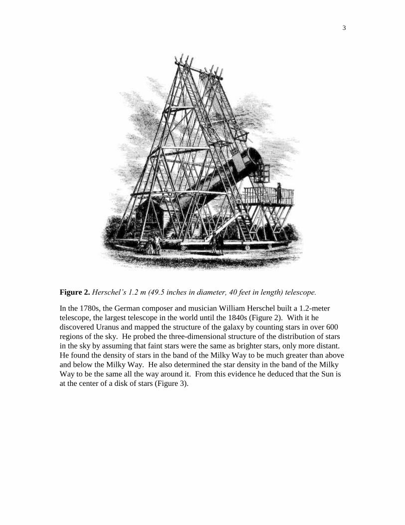
Figure 2. Herschel’s 1.2 m (49.5 inches in diameter, 40 feet in length) telescope.

In the 1780s, the German composer and musician William Herschel built a 1.2-meter

telescope, the largest telescope in the world until the 1840s (Figure 2). With it he

discovered Uranus and mapped the structure of the galaxy by counting stars in over 600

regions of the sky. He probed the three-dimensional structure of the distribution of stars

in the sky by assuming that faint stars were the same as brighter stars, only more distant.

He found the density of stars in the band of the Milky Way to be much greater than above

and below the Milky Way. He also determined the star density in the band of the Milky

Way to be the same all the way around it. From this evidence he deduced that the Sun is

at the center of a disk of stars (Figure 3).

4

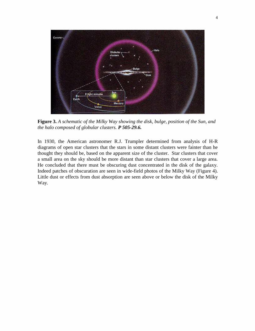
Figure 3. A schematic of the Milky Way showing the disk, bulge, position of the Sun, and

the halo composed of globular clusters. P 505-29.6.

In 1930, the American astronomer R.J. Trumpler determined from analysis of H-R

diagrams of open star clusters that the stars in some distant clusters were fainter than he

thought they should be, based on the apparent size of the cluster. Star clusters that cover

a small area on the sky should be more distant than star clusters that cover a large area.

He concluded that there must be obscuring dust concentrated in the disk of the galaxy.

Indeed patches of obscuration are seen in wide-field photos of the Milky Way (Figure 4).

Little dust or effects from dust absorption are seen above or below the disk of the Milky

Way.

5

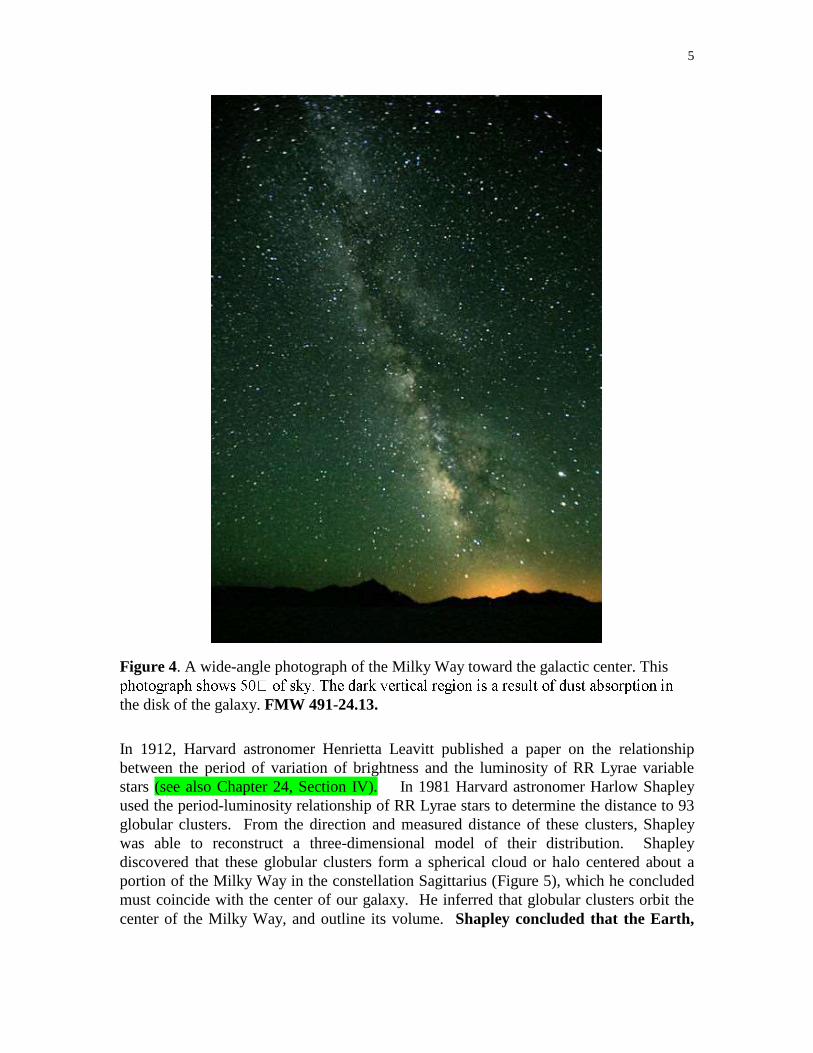
Figure 4. A wide-angle photograph of the Milky Way toward the galactic center. This

the disk of the galaxy. FMW 491-24.13.

In 1912, Harvard astronomer Henrietta Leavitt published a paper on the relationship

between the period of variation of brightness and the luminosity of RR Lyrae variable

stars (see also Chapter 24, Section IV). In 1981 Harvard astronomer Harlow Shapley

used the period-luminosity relationship of RR Lyrae stars to determine the distance to 93

globular clusters. From the direction and measured distance of these clusters, Shapley

was able to reconstruct a three-dimensional model of their distribution. Shapley

discovered that these globular clusters form a spherical cloud or halo centered about a

portion of the Milky Way in the constellation Sagittarius (Figure 5), which he concluded

must coincide with the center of our galaxy. He inferred that globular clusters orbit the

center of the Milky Way, and outline its volume. Shapley concluded that the Earth,

6

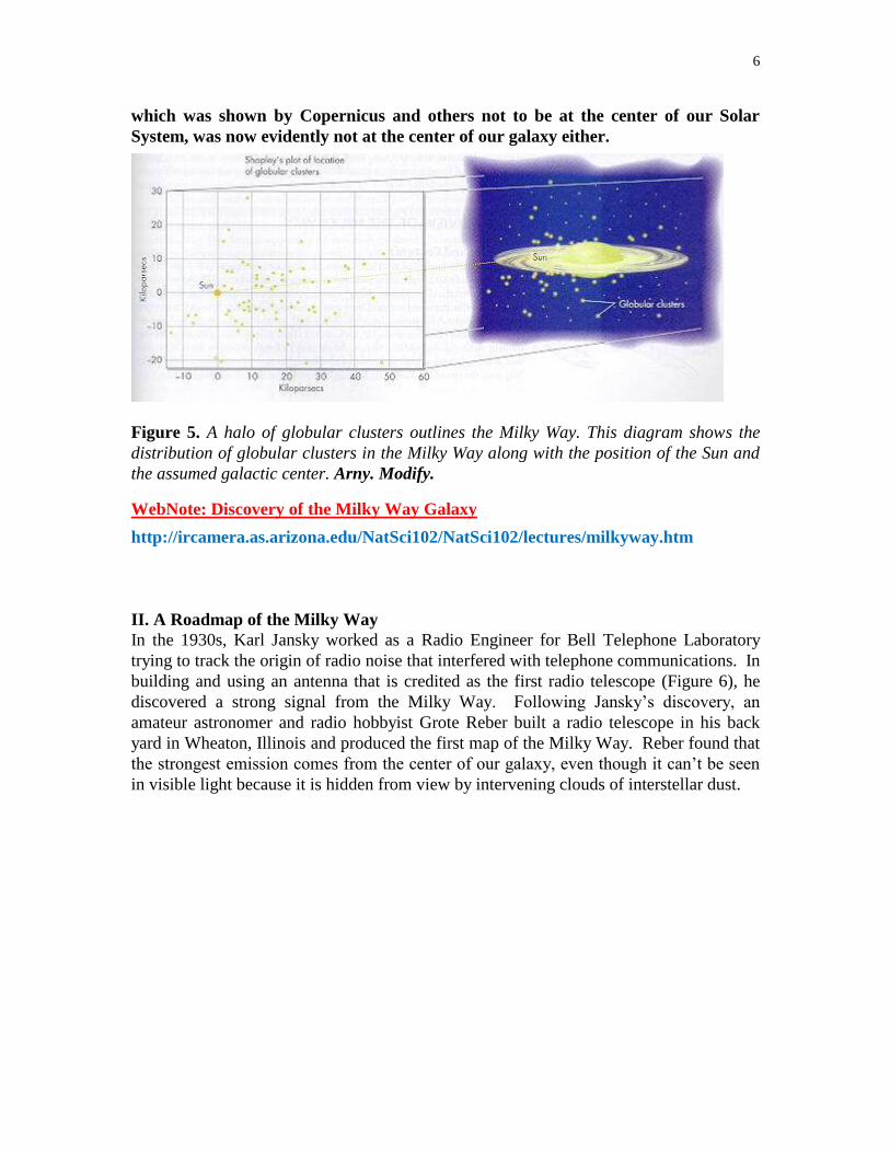
which was shown by Copernicus and others not to be at the center of our Solar

System, was now evidently not at the center of our galaxy either.

Figure 5. A halo of globular clusters outlines the Milky Way. This diagram shows the

distribution of globular clusters in the Milky Way along with the position of the Sun and

the assumed galactic center. Arny. Modify.

WebNote: Discovery of the Milky Way Galaxy

http://ircamera.as.arizona.edu/NatSci102/NatSci102/lectures/milkyway.htm

II. A Roadmap of the Milky Way

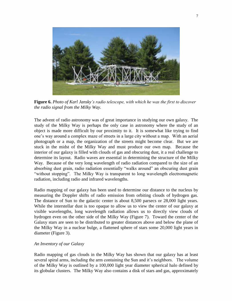
In the 1930s, Karl Jansky worked as a Radio Engineer for Bell Telephone Laboratory

trying to track the origin of radio noise that interfered with telephone communications. In

building and using an antenna that is credited as the first radio telescope (Figure 6), he

discovered a strong signal from the Milky Way. Following Jansky’s discovery, an

amateur astronomer and radio hobbyist Grote Reber built a radio telescope in his back

yard in Wheaton, Illinois and produced the first map of the Milky Way. Reber found that

the strongest emission comes from the center of our galaxy, even though it can’t be seen

in visible light because it is hidden from view by intervening clouds of interstellar dust.

7

Figure 6. Photo of Karl Jansky’s radio telescope, with which he was the first to discover

the radio signal from the Milky Way.

The advent of radio astronomy was of great importance in studying our own galaxy. The

study of the Milky Way is perhaps the only case in astronomy where the study of an

object is made more difficult by our proximity to it. It is somewhat like trying to find

one’s way around a complex maze of streets in a large city without a map. With an aerial

photograph or a map, the organization of the streets might become clear. But we are

stuck in the midst of the Milky Way and must produce our own map. Because the

interior of our galaxy is filled with clouds of gas and obscuring dust, it a real challenge to

determine its layout. Radio waves are essential in determining the structure of the Milky

Way. Because of the very long wavelength of radio radiation compared to the size of an

absorbing dust grain, radio radiation essentially “walks around” an obscuring dust grain

“without stopping”. The Milky Way is transparent to long wavelength electromagnetic

radiation, including radio and infrared wavelengths.

Radio mapping of our galaxy has been used to determine our distance to the nucleus by

measuring the Doppler shifts of radio emission from orbiting clouds of hydrogen gas.

The distance of Sun to the galactic center is about 8,500 parsecs or 28,000 light years.

While the interstellar dust is too opaque to allow us to view the center of our galaxy at

visible wavelengths, long wavelength radiation allows us to directly view clouds of

hydrogen even on the other side of the Milky Way (Figure 7). Toward the center of the

Galaxy stars are seen to be distributed to greater distances above and below the plane of

the Milky Way in a nuclear bulge, a flattened sphere of stars some 20,000 light years in

diameter (Figure 3).

An Inventory of our Galaxy

Radio mapping of gas clouds in the Milky Way has shown that our galaxy has at least

several spiral arms, including the arm containing the Sun and it’s neighbors. The volume

of the Milky Way is outlined by a 100,000 light year diameter spherical halo defined by

its globular clusters. The Milky Way also contains a disk of stars and gas, approximately

8

100,000 light years in diameter and 2,000 light years thick, centered in the galactic halo

(Figure 3).

The galactic disk contains open star clusters, OB associations, and unassociated stars,

also called field stars. Filling the void in between these stars is the so-called interstellar

medium, dust and gas; the latter exists in both atomic and molecular form. Hydrogen gas

is usually found in atomic form if it is bathed in the warmth of nearby stars and is in

molecular form in the dark confines of cold, relatively dense clouds of gas and dust. The

density of gas and dust in the interstellar medium, even in giant molecular clouds, is so

low, that it is an excellent vacuum by Earth-laboratory standards. Interstellar dust is

composed of the same materials that made up dust in the early Solar System, water,

ammonia, and methane ices, silicates, and iron.

The evidence of gas and dust in the Milky Way are the infrared emission and the emission

lines from atomic gas seen in hot, star-illuminated dust and gas clouds, and the gas

absorption lines and dust obscuration imposed on stars in the Milky Way by intervening

gas and dust (Figure 8).

Figure 7. A 21-cm map of the sky shows the distribution of cold hydrogen in the Milky

Way. This false color map shows the most intense emission corresponding to the lightest

colors in the plane of the Milky Way and the least intense emission corresponding to the

darkest colors in the directions perpendicular to the plane of our galaxy. FMW 485-24.8

& APOD.

9

Figure 8. An infrared image of the sky from the Cosmic Background Explorer satellite.

This false-color image shows the infrared emission from the disk and bulge of our own

Milky Way. NASA. APOD.

Multiple Wavelength Images of the Milky Way and the Whirlpool Galaxy1

“Galaxies are complex systems composed of many different components, including high

and low mass stars, star clusters and associations, gaseous nebulae, and dust. These

components are not all uniquely detected from observations in the same part of the

electromagnetic spectrum (Table 21.1, Figure 9). For example, to detect an extremely hot

star with a surface temperature of 20,000 K, a detector highly sensitive to the ultraviolet

region of the spectrum would be desirable, since the wavelength of maximum intensity of

a 20,000 K blackbody is approximately 150 nanometers (10-9

m). One can determine the

most sensitive wavelength regions to detect thermal sources (those having blackbody-like

spectra), such as stars or cold dust, by using Wien’s law, max = 2.898 x 106/T, where

max is the wavelength of maximum intensity in nanometers and T is the effective

(photospheric or surface) temperature of the object in Kelvins (Table 21.2).

1 From Laboratory Experiments for Astronomy, by Johnson & Canterna

10

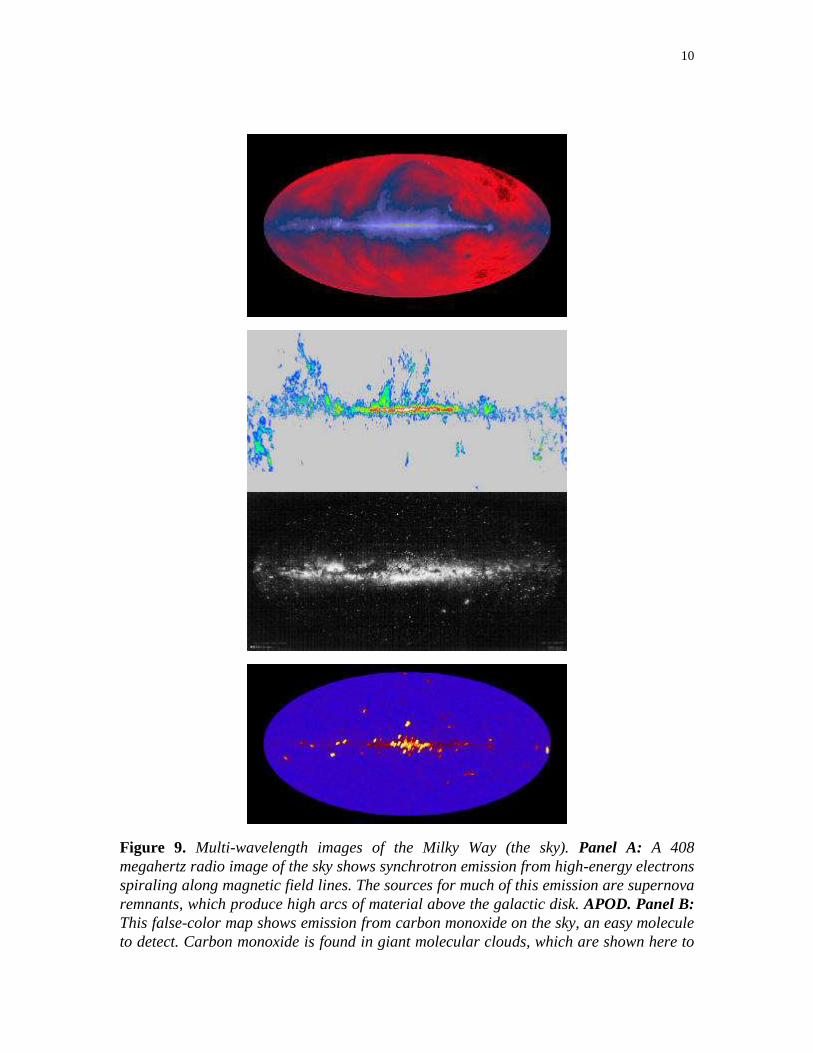
Figure 9. Multi-wavelength images of the Milky Way (the sky). Panel A: A 408

megahertz radio image of the sky shows synchrotron emission from high-energy electrons

spiraling along magnetic field lines. The sources for much of this emission are supernova

remnants, which produce high arcs of material above the galactic disk. APOD. Panel B:

This false-color map shows emission from carbon monoxide on the sky, an easy molecule

to detect. Carbon monoxide is found in giant molecular clouds, which are shown here to

11

be concentrated in the disk of the Milky Way.. APOD. Panel C: A drawing of the Milky

Way made under the direction of Knut Lundmark. This drawing shows the distribution of

over 7,000 bright stars and dust clouds that obscure starlight. Panel D: A map of the X-

ray emission from the sky. Most of this emission comes from white dwarfs, neutron stars,

and black holes in the Milky Way. APOD.

Figure 10. Multi-wavelength images of the Whirlpool Galaxy. Panel A: A false color

image of 21-cm radio emission from hydrogen gas. Arny. Panel B: A visible image color

image. Panel C: An ISO (Infrared Space Observatory) infrared image showing the

locations of warm dust illuminated by starlight. Panel D: A false-color radio telescope

image of M51 at a wavelength that captures emission from carbon monoxide molecules in

giant molecular clouds. P-546-33.3.

“For non-blackbody sources, such as ionized hydrogen (HII) regions or planetary nebulae,

a similar technique is used. These gaseous nebulae are strong emission line sources. One

of the strongest emission lines from HII regions is the red Balmer line of hydrogen (H).

A photograph or image of a galaxy using a narrow filter that transmits energy around H

will record the presence of HII regions since the H line is very strong.

“Care must be taken with the interpretation of these filtered images. Not only will an HII

region appear bright on an H image, but also stars, owing to their thermal emission, will

emit energy in this wavelength region and register on an image. The key toward a proper

interpretation of the data is given in the following explanation. For a given exposure

time, it may take 1,000-10,000 stars to produce the same brightness per unit area as a

12

given HII region in H light, powered by only a few stars. For regions with a high

density of stars, additional criteria must be used to differentiate between H and thermal

emission. Generally additional images in other emission lines or the spatial appearance

of the H image are used. This will become more apparent when we examine the H

image of the Whirlpool Galaxy (Figure 10).

Table 21.1: Galactic Components

Typical Object Temperature max

High mass star ~10,000 K 350 nm

1 solar mass star 5,800 K 550 nm

Low mass star ~2,500 K 1000 nm (1 micron)

Cold dust ~25 K 100 microns

Neutral H gas -- 21 cm

Ionized H -- H

Table 21.2: Stellar Temperature Classes

Class Temperature max

O > 25,000 K Ultraviolet

B 11,000 – 25,000 K Ultraviolet

A 7,5000 – 11,000 K Blue

F 6,000 – 7,500 K White to blue

G 5,000 – 6,000 K Yellow to white

K 3,500 – 5,000 K Red to orange

M < 3,500 K Infrared to red

Webnote: Mapping Populations in M51 at Different Wavelengths

http://coolcosmos.ipac.caltech.edu/cosmic_classroom/multiwavelength_astronomy/m

ultiwavelength_museum/m51.html

http://ircamera.as.arizona.edu/NatSci102/NatSci102/lectures/milkywayparts.htm

III. Other Galaxies

Until 1924 many astronomers thought that some spiral nebulae, seen as blurred patches

with a spiral structure, were in the Milky Way, much like the Orion nebula is seen to be

close by. However, in 1924 the new 100-inch telescope on Mt. Wilson in California

produced photographs of the spiral Andromeda galaxy that showed that this galaxy

consisted of an uncountable number of faint stars. Later, the period-luminosity

relationship of variable stars were used to determine that Andromeda has a distance of 2

million light years, well outside of the Milky Way.

13

IV. Radio Observations and Spiral Structure

Radio observations not only allow astronomers to “look around” the dust, but also allow

them to construct three-dimensional maps of the concentrations of gas that form the spiral

arms.

One of the most useful radio wavelengths for mapping the Milky Way is 21-centimeters,

the wavelength at which cold unionized (or “neutral”) hydrogen emits. Neutral hydrogen

consists of a proton orbited by a single electron. In addition to the orbital motion of the

electron, both the proton and electron are spinning. For each energy level of the hydrogen

atom, the electron has two possible states. Its spin is either in the same direction as that

of its proton, or it is in the opposite direction. If the electron flips from one state to the

other it can emit or absorb a tiny amount of energy (Figure 11). This energy has a

wavelength of 21-centimeters. Because hydrogen is found everywhere in the galaxy and

dust clouds are transparent to 21-centimeter radiation, this wavelength is the staple of the

radio astronomer.

Figure 11. Twenty-one-cm emission from the electron spin-flip in hydrogen. When the

electron orbiting the nucleus of a hydrogen atom flips, from spinning in the same

direction as the nucleus to spinning in the opposite direction, the atom gives off a low-

energy photon with a wavelength of 21 centimeters. P 526-30.11, top half only.

Figure 12. Mapping the structure of the Milky Way with 21-cm hydrogen emission. The

relative distance to a hydrogen cloud orbiting the center of the Milky Way can be

determined from the Doppler shift of its 21-cm emission, which is determined by its

velocity along the line of sight. Cloud C is moving away from the Sun in its orbit, and so

it appears red shifted. Cloud A appears to be moving toward the Sun so its emission is

blue shifted. Objects in line with the galactic center, B1 and B2, have no line of sight

14

velocity with respect to the Sun and thus no Doppler shift. The closer a hydrogen cloud is

to the Milky Way nucleus the greater its orbital velocity. This information can be used to

piece together a three-dimensional hydrogen emission map of the galaxy. P 528-30.13.

21-centimeter emission was first used to map the Milky Way in 1951. Although the

visible sky appears only 2-dimensional, astronomers use a trick to construct a three-

dimensional map of the Galaxy. Astronomers can point a radio telescope at a gas cloud

and determine its direction in space. But how far away is it? This information can be

found from the Doppler shift of the 21-centimeter hydrogen emission. If hydrogen gas in

the disk of the Milky Way is orbiting the center of the Milky Way in circular orbits which

obey Kepler’s 3rd

law (the more distant the gas, the slower it orbits), then the astronomer

can determine its distance from how fast it is moving away from or toward the Sun (us)

(Figure 12). Different Doppler shifts correspond to different distances.

Once a 3-dimensional map of hydrogen emission is constructed, what does it show?

Maps show a number of arcs of neutral hydrogen giving us a suggestion of spiral structure

(Figure 13). In other galaxies we see spiral arms that are outlined by bright blue young

stars and emission nebulae, giant molecular clouds, and OB associations, places where

massive stars are forming (Figure 10).

Figure 13. Schematic of spiral arms in the Milky Way. Modify. Hartmann and Impey.

15

Although dust limits our view of the Milky Way, radio observations and infrared images

allow observations past 23,000 parsecs (75,000 light years) from the galactic center.

These show that the Milky Way has spiral arms and arm segments. Our Sun is located on

the inner edge in a short arm segment including the Orion nebula, called the Orion arm

(Figure 13). Adjacent to the Orion arm are the Perseus arm and Sagittarius arm, which

contain the stars prominent in these constellations.

V. Spiral Structure

Spiral galaxies are defined by the beautiful arms that grace them. Spiral arms are outlined

by HII regions and the luminous blue stars in OB associations. Spiral galaxies are

usually divided into two classes, flocculent and grand-design. Flocculent (or “fleecy”)

spirals are characterized by ill-defined spiral arms, a seemingly random array of

numerous short spiral arm segments, whereas grand-design galaxies have a small number,

as few as two, of long, continuous, well-defined spiral arms (Figure 14).

16

Figure 14. Images of a flocculent (M33, above) and a grand-design spiral (NGC 2997,

below). Wikimedia Commons; Malin & AAT.

What causes this spiral structure? The cause of spiral arms has been a great mystery of

astronomy until the 1960s. Simplistic ideas based on the formation of a linear arm that is

stretched into a spiral arm as a result of differential rotation fail. The reason for the

failure of simple rotation models is the problem with spiral arms “winding up” in a

relatively short time (Figure 15). Because disk stars orbit the nucleus of the Milky Way

in nearly circular orbits, governed by Kepler’s laws, the farther a star is from the center of

the Milky Way, the longer its orbital period. This same phenomenon is seen in planets; it

takes longer for Pluto to orbit the Sun than it does the Earth. In the 5 billion-year lifetime

of the Sun, it has orbited the Milky Way nucleus about 25 times. The Sun is part of the

Orion spiral arm. This spiral arm would have wound up so tightly in 5 billion years as to

be totally unrecognizable as a spiral arm. Arms in galaxies are not tightly wound but are

relaxed gently curving arms. How can these arms be explained?

17

We only see spiral arms because of the blue massive stars strung along them.

Surprisingly, the spiral arms contain only 5% more stars than the regions between the

arms. The lower mass solar-type stars are evenly distributed throughout the disk. The

spiral arms are visually distinguished from the inter-arm regions as the recent sites of

high-mass star formation. There are two theories used to explain the enhanced star

formation along spiral arms: density wave theory and self-propagating star formation.

Density Wave Theory

In the 1920s the Swedish Astronomer, Bertil Lindblad, suggested that compression waves

traveling through a rotating disk are the cause of spiral arms (Figures 16). American

astronomers C.C. Lin and Frank Shu refined this theory in the 1960s with the aid of

modern computers. Ripples in a rotating galaxy, much like ripples in a rotating pan of

water, would be spiral shaped. As spiral compression waves move through a galaxy,

material at the wave crests is compressed and becomes locally more dense. The waves

are not associated with any particular stars or giant molecular clouds, but move through

them as a sound wave moves through air or a ripple moves through water in a pond. As

the compression wave moves through giant molecular clouds it compresses them, seeding

their collapse and initiating star formation.

Figure 15. The windup problem in spiral arm formation. This imaginary time sequence

shows how large molecular clouds would become elongated due to the differential

rotation of the galaxy. The inner parts rotate the fastest, eventually winding up the clouds

through many rotations into arms that are so tightly wound that they would not be

recognizable. FMW 486-24.10 modified.

Why don’t the spiral arms wind-up in the density wave model? High-mass stars live only

for tens of millions of years. It takes the Sun approximately 200 million years to orbit the

center of the Milky Way once. A high-mass blue star with a 10 million-year lifetime will

only move through a short segment of its orbit over its life. As the spiral density wave

moves slowly through the galaxy, luminous high-mass stars are born when the crest of the

density wave piles into a giant molecular cloud. By the time the density wave moves on,

the high-mass star has already died. HII regions, OB associations, and short-lived stars

will be seen only at the crest of the density wave. Other more long-lived objects are left

behind the crest and live their lives long after the spiral wave has passed. In this model a

spiral arm is an arm of recent star formation.

18

What is the mechanism for starting a compression wave? It could be the gravitational

interaction with a nearby or companion galaxy. Like plucking a guitar string a passing

galaxy pulls on its neighbor with its gravity. The neighbor responds by the propagation

of a spiral density wave, just as a pond ripples when a stone is dropped into it.

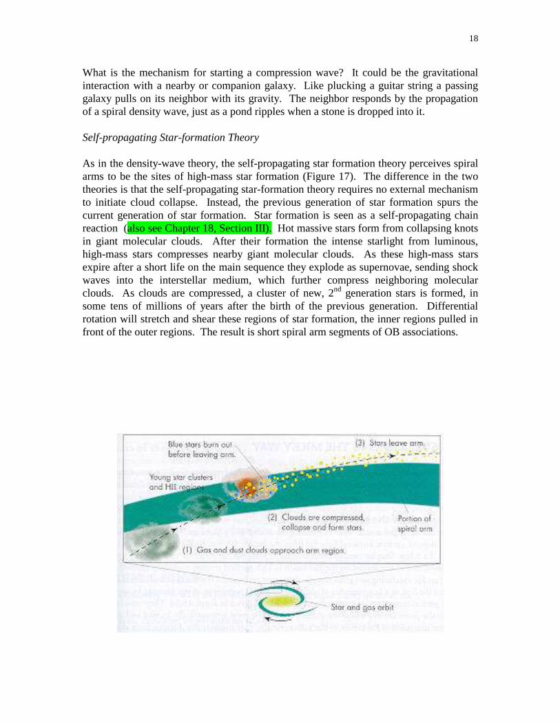
Self-propagating Star-formation Theory

As in the density-wave theory, the self-propagating star formation theory perceives spiral

arms to be the sites of high-mass star formation (Figure 17). The difference in the two

theories is that the self-propagating star-formation theory requires no external mechanism

to initiate cloud collapse. Instead, the previous generation of star formation spurs the

current generation of star formation. Star formation is seen as a self-propagating chain

reaction (also see Chapter 18, Section III). Hot massive stars form from collapsing knots

in giant molecular clouds. After their formation the intense starlight from luminous,

high-mass stars compresses nearby giant molecular clouds. As these high-mass stars

expire after a short life on the main sequence they explode as supernovae, sending shock

waves into the interstellar medium, which further compress neighboring molecular

clouds. As clouds are compressed, a cluster of new, 2nd

generation stars is formed, in

some tens of millions of years after the birth of the previous generation. Differential

rotation will stretch and shear these regions of star formation, the inner regions pulled in

front of the outer regions. The result is short spiral arm segments of OB associations.

19

Figure 16. Density wave theory schematic showing star formation as a giant molecular

cloud moves through a density wave. Arny. Modify.

Figure 17. Self-propagating star formation in a molecular cloud. A bright open cluster is

seen on the left. Intense light originating from this cluster as well as compression waves

from supernovae in the cluster serve to compress the rest of the molecular cloud. The

result is the formation of protostars on the right side of the cloud. P 535-30.24 modified.

WebAnimation: Spiral Arm Formation Simulation

http://www.youtube.com/watch?v=hVNuwAtnKeg

What are the pros and cons of each model? In the self-propagating star-formation

model, random bursts of star formation would result in the appearance and disappearance

of short arm segments, of the type seen in flocculent spiral galaxies. The grand-design

spirals are more satisfactorily explained by density wave theory, which can account for

the longer more distinct spiral arms. Perhaps the difference in the appearance of these

two types of galaxies can be accounted for by whether or not a galaxy has had a close

encounter with a neighboring galaxy in the recent past.

VI. Mass of the Milky Way

Orbital motion of stars and gas about the center of mass of the Milky Way has kept them

from falling into its center billions of years ago just as the Moon’s circular orbit about the

Earth has kept it from falling into our planet. Their motion, as has been determined by

Doppler shift measurements, indicates that the Milky Way does not rotate like a rigid

body, like a phonograph record on a turntable, but by differential rotation, much as the

planets orbit the Sun.

The Sun travels around the center of the galaxy at 828,000 km/hour (225 km/s), but

because of the enormous size of the Milky Way it takes about 230 million years to

20

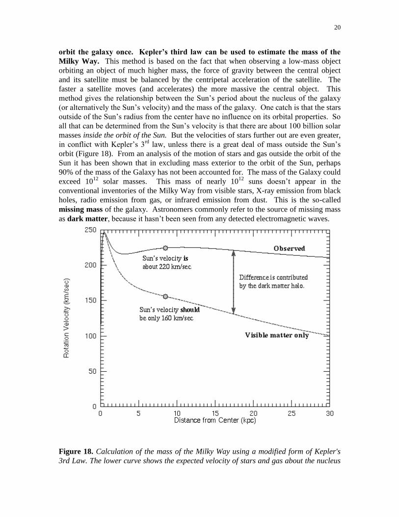
orbit the galaxy once. Kepler’s third law can be used to estimate the mass of the

Milky Way. This method is based on the fact that when observing a low-mass object

orbiting an object of much higher mass, the force of gravity between the central object

and its satellite must be balanced by the centripetal acceleration of the satellite. The

faster a satellite moves (and accelerates) the more massive the central object. This

method gives the relationship between the Sun’s period about the nucleus of the galaxy

(or alternatively the Sun’s velocity) and the mass of the galaxy. One catch is that the stars

outside of the Sun’s radius from the center have no influence on its orbital properties. So

all that can be determined from the Sun’s velocity is that there are about 100 billion solar

masses inside the orbit of the Sun. But the velocities of stars further out are even greater,

in conflict with Kepler’s 3rd

law, unless there is a great deal of mass outside the Sun’s

orbit (Figure 18). From an analysis of the motion of stars and gas outside the orbit of the

Sun it has been shown that in excluding mass exterior to the orbit of the Sun, perhaps

90% of the mass of the Galaxy has not been accounted for. The mass of the Galaxy could

exceed 1012

solar masses. This mass of nearly 1012

suns doesn’t appear in the

conventional inventories of the Milky Way from visible stars, X-ray emission from black

holes, radio emission from gas, or infrared emission from dust. This is the so-called

missing mass of the galaxy. Astronomers commonly refer to the source of missing mass

as dark matter, because it hasn’t been seen from any detected electromagnetic waves.

Figure 18. Calculation of the mass of the Milky Way using a modified form of Kepler's

3rd Law. The lower curve shows the expected velocity of stars and gas about the nucleus

21

of the Milky Way vs. distance from the galactic center, using an estimate of the mass of

the Milky Way from visible matter (stars, gas clouds, and dust). The lower curve

represents the measured velocity vs. radial distance curve for the Milky Way. The

displacement between the two curves indicates a substantial unseen or "missing" mass in

the Milky Way. Modify. Nick Stroebel's Web site.

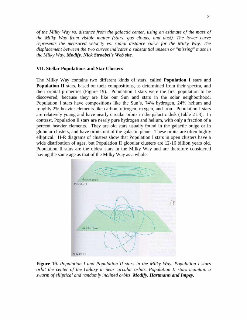
VII. Stellar Populations and Star Clusters

The Milky Way contains two different kinds of stars, called Population I stars and

Population II stars, based on their compositions, as determined from their spectra, and

their orbital properties (Figure 19). Population I stars were the first population to be

discovered, because they are like our Sun and stars in the solar neighborhood.

Population I stars have compositions like the Sun’s, 74% hydrogen, 24% helium and

roughly 2% heavier elements like carbon, nitrogen, oxygen, and iron. Population I stars

are relatively young and have nearly circular orbits in the galactic disk (Table 21.3). In

contrast, Population II stars are nearly pure hydrogen and helium, with only a fraction of a

percent heavier elements. They are old stars usually found in the galactic bulge or in

globular clusters, and have orbits out of the galactic plane. These orbits are often highly

elliptical. H-R diagrams of clusters show that Population I stars in open clusters have a

wide distribution of ages, but Population II globular clusters are 12-16 billion years old.

Population II stars are the oldest stars in the Milky Way and are therefore considered

having the same age as that of the Milky Way as a whole.

Figure 19. Population I and Population II stars in the Milky Way. Population I stars

orbit the center of the Galaxy in near circular orbits. Population II stars maintain a

swarm of elliptical and randomly inclined orbits. Modify. Hartmann and Impey.

22

Table 21.3: Properties of Stellar Populations

Population I Population II

Distribution In spiral arms, patchy

distribution

Smooth distribution in halo

Heavy Element

Abundance

2-4% 0.1%

Ages 0 – 1010

years 1010

years

Orbits Circular Elliptical

Objects Open clusters, OB

associations, star formation

regions

Globular clusters

IIX. Origin of the Milky Way Galaxy

It is thought that the Milky Way formed from a rotating, fragmenting cloud of self-

gravitating gas, similar to the way that individual stars and star clusters are thought to

have formed, but on a much larger scale (Figure 20). Originally the cloud that formed our

galaxy was composed of 75% hydrogen and 25% helium, by mass, with no significant

contribution from heavier elements. The volume of the cloud is presumed to match the

volume currently occupied by globular clusters. About 13 billion years ago, the age of

the oldest globular clusters, the galactic gas cloud began to collapse and fragment,

forming stars throughout the entire galactic volume. The globular clusters maintained

orbits about the center of mass of the galaxy while the gas collapsed into a rotating disk,

much as a collapsing presolar cloud collapsed into a Sun surrounded by a spinning dust

disk (Chapter 12, Section V). The stars that formed prior to galactic disk collapse are the

Population II stars in the Galaxy. (Remember: Population II stars formed first.)

23

Figure 20. Formation of the Milky Way. In a simple model, the Galaxy is formed by the

collapse of a giant gas cloud (1). The first objects to condense out of the collapsing

protogalactic cloud are globular clusters (2). The underlying gas continues to collapse to

a disk (3). Star formation continues in the disk from gas that had been enriched with

metals from the stars that had already formed in the halo (4). FMW 494-24.17.

In the second phase of the formation of the Galaxy, a spinning disk of gas formed and

Population I stars began to form in the disk. The first generation of stars started brewing

heavier elements in their interiors with thermonuclear fusion. As these stars died they

began to recycle heavier elements back into the interstellar medium, out of which the

newer stellar generations would form. Recycling into the interstellar medium then took

place via planetary nebulae, supernovae, stellar winds, and binary mass exchange

(Chapter 19, Section III). Subsequently, newer generations of stars came and went,

enhancing the heavy elements in the interstellar medium.

The proposed scenario, while it explains the gross properties of our galaxy, isn’t perfect.

There are problems with some of the details. For example, the predicted free-fall time for

the collapse of the galactic gas cloud is several hundred million years. However, this

doesn’t match the 3 billion-year spread in globular cluster ages as determined from their

H-R diagrams. It will take a more complex and comprehensive model to explain more of

the observed details of our galaxy.

IX. The Nucleus

The density of stars at the center of the Milky Way is so great that if you lived on a planet

orbiting a star at the center of the Galaxy you would see 1 million stars as bright as Sirius,

one of the brightest stars in our sky. It would never really get dark at night. But the

nucleus of our galaxy is unusually luminous in the radio and infrared regions of the

spectrum as well. The visible dust between the galactic nucleus and the Sun totally

prevents us from seeing any of the stars at the nucleus of the galaxy. With infrared light

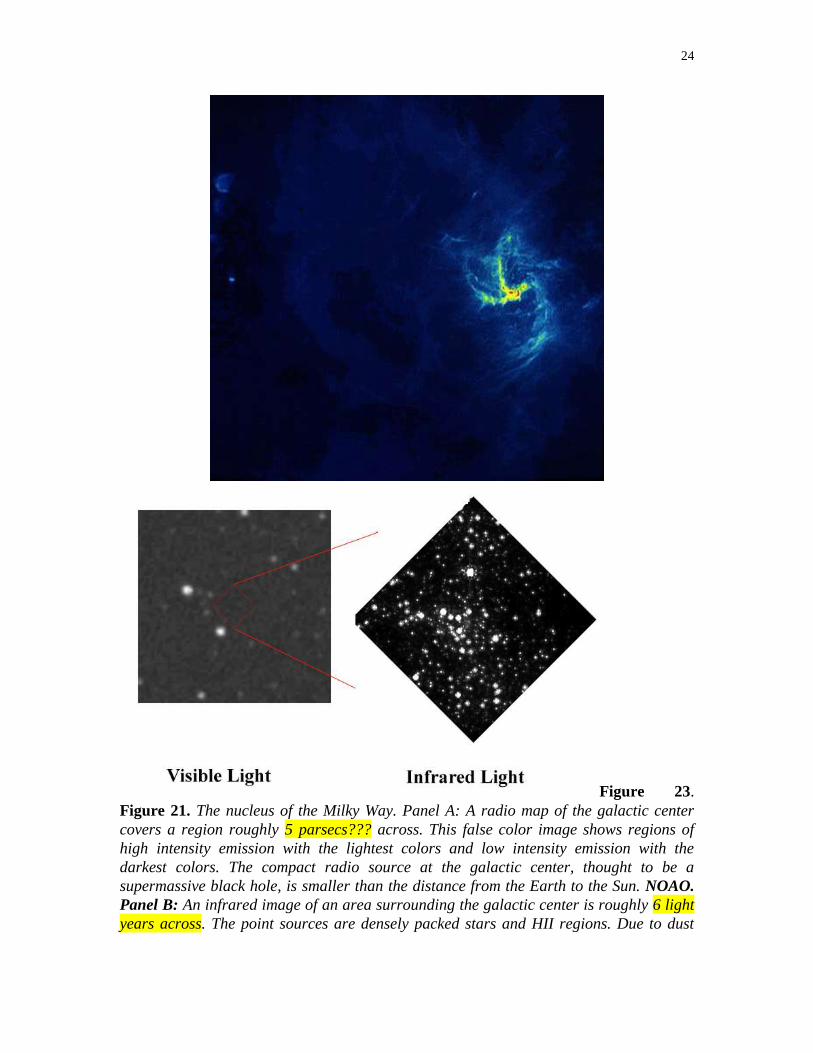
and radio radiation we can see an exposed galactic center (Figure 21).

24

Figure 23.

Figure 21. The nucleus of the Milky Way. Panel A: A radio map of the galactic center

covers a region roughly 5 parsecs??? across. This false color image shows regions of

high intensity emission with the lightest colors and low intensity emission with the

darkest colors. The compact radio source at the galactic center, thought to be a

supermassive black hole, is smaller than the distance from the Earth to the Sun. NOAO.

Panel B: An infrared image of an area surrounding the galactic center is roughly 6 light

years across. The point sources are densely packed stars and HII regions. Due to dust

25

obscuration, these objects cannot be seen in visible light. From

http://ircamera.as.arizona.edu/NatSci102/NatSci102/lectures/galcenter.htm.

Figure 22. Schematic of the Milky Way nucleus. Arny. Modify.

Strong infrared emission comes from a group of several powerful radio emitters at the

galactic center, called Sagittarius A (Figure 22). Sagittarius A is one of the brightest

sources of synchrotron emission in the sky. Synchrotron emission is the emission of

electromagnetic radiation from electrons spiraling in a magnetic field, the same kind of

emission that produces the Earth’s aurorae.

The most luminous of the Sagittarius A radio sources is called Sagittarius A*, thought to

be the nucleus of our galaxy. Two arms of hydrogen gas have been detected by 21-cm

emission that originate in the nucleus; one is approaching us at 53 km/s and another

receding at 135 km/s. The length and velocity of these arms indicate that they were

blown out of the galactic core about 10 million years ago.

In addition to these arms, there is a ring of gas orbiting the galactic center. Doppler shifts

of broadened neon gas indicate that gas is orbiting the nucleus at up to 200 km/s. From

this Kepler’s 3rd

law indicates 1 million solar masses of matter in a region smaller than a

few light-years across. Most think that this mass is contained in a supermassive black

hole with a hot accretion disk causing emission in the radio and infrared. This kind of

black hole-like activity is seen in other galaxy nuclei as well. Matter is expected to fall to

the center of the Galaxy as it collapses and forms stars, and would naturally form a

supermassive black hole at the Galaxy nucleus.

Webnote: The Galactic Center

http://ircamera.as.arizona.edu/NatSci102/NatSci102/lectures/galcenter.htm

26

Summary

The Milky Way, like other spiral galaxies, is a dense disk of stars, about 100,00 light

years in diameter, surrounded by a spherical halo of globular clusters. Luminous, blue

stars outline a spiral pattern in the disk. The Sun is embedded in such a spiral arm, about

two-thirds the distance from the center of the Galaxy to the edge of the disk. One of the

most useful methods of mapping the structure of the Milky Way uses the 21-cm emission

line of hydrogen, due to the spin-flip of the single hydrogen electron. The disk of the

Milky Way consists of stars and gas clouds independently orbiting the galactic center.

Use of Kepler’s 3rd

law allows us to estimate the mass of the Milky Way from

measurements of their velocities about the nucleus. There are two theories of spiral arm

formation in galaxies like the Milky Way. The first is the density wave theory, in which

spiral waves of mass density propagate through the disk, compressing gas clouds and

instigating star formation. The second is the self-propagating star formation theory in

which a high mass star evolves and supernovas; the resulting compression wave collapses

gas clouds and initiates star formation in them. The resulting pattern of star formation in

a rotating galaxy is spiral. The Milky Way and other spirals contain two populations of

stars, old Population II stars and younger Population I stars. Population I stars fill the

disk including the spiral arms. Population II stars are seen in the galaxy halo and central

bulge. The nucleus of the Milky Way is a source of energetic activity indicating the likely

existence of a black hole and high temperature accretion disk.

Key Words & Phrases

1. Density wave theory – a theory of spiral arm formation based on the idea of spiral

compression waves moving through the galaxy inducing star formation

2. Field star – a star which is not a member of a cluster or association

3. Flocculent spiral – a spiral galaxy which has short, patchy spiral arm segments

4. Grand-design spiral – a spiral galaxy which has long, distinct spiral arms

5. Interstellar medium – the space between stars in a galaxy, which is filled with gas

and dust

6. Milky Way – our own galaxy

7. Population I stars – the metal-rich population of stars, preferentially found in the

galactic disk

8. Population II stars – the old, metal-poor population of stars, found chiefly in the

galactic halo

9. RR Lyrae variable

10. Self-propagating star formation – a theory of spiral arm formation based on the

idea of a previous generation of star formation inducing a second wave of star

formation from supernova shock waves and intense radiation pressure. The resulting

regions of young stars are then stretched by differential rotation into spiral arm

segments.

27

11. Synchrotron emission - the emission of electromagnetic radiation from electrons

spiraling in a magnetic field, the same kind of emission that produces the Earth’s

aurorae

Review for Understanding

1. Why do we think that our galaxy is a spiral?

2. Sketch (a) a side view and (b) a top view of the Milky Way, showing the shapes and

relative sizes of the nucleus, disk, halo, and position of the Sun.

3. How do we know the size of the Galaxy? The location of the center?

4. How do we know the mass of the Galaxy?

5. What are the spiral arms of the Galaxy made of?

6. Why does the Galaxy have spiral arms?

Essay Questions

1. How do stars orbit the Galaxy?

28

_______________________________________________________________________

Chapter 22 – Normal Galaxies

It is not too much to say that the understanding of why there are these different kinds of

galaxy, of how galaxies originate, constitutes the biggest problem in present-day

astronomy. The properties of the individual stars that make up the galaxies form the

classical study of astrophysics, while the phenomenon of galaxy formation, touches on

cosmology. In fact, the study of galaxies forms a bridge between conventional astronomy

and astrophysics on the one hand, and cosmology on the other.

--Fred Hoyle, Galaxies, Nuclei, and Quasars, 1965

Chapter Preview

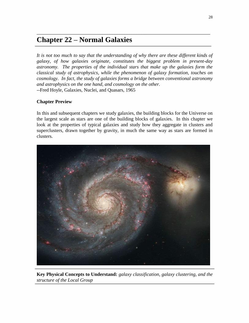
In this and subsequent chapters we study galaxies, the building blocks for the Universe on

the largest scale as stars are one of the building blocks of galaxies. In this chapter we

look at the properties of typical galaxies and study how they aggregate in clusters and

superclusters, drawn together by gravity, in much the same way as stars are formed in

clusters.

Key Physical Concepts to Understand: galaxy classification, galaxy clustering, and the

structure of the Local Group

29

I. Discovery of Galaxies

Until the early part of this century astronomers thought that the Milky Way galaxy was

the entire Universe. Indeed, only a handful of celestial bodies viewable with the unaided

eye are outside the Milky Way, including the Andromeda Galaxy and the Large and Small

Magellanic Clouds. It wasn’t until 300 hundred years after the invention of the telescope

that the location of galaxies, whether interior or exterior to the Milky Way, became a

controversial issue.

In 1755, the German philosopher Immanuel Kant proposed that there were groups of stars

beyond the Milky Way which he called “island universes”. The Irish astronomer William

Parsons, the 3rd

Earl of Rosse, used his wealth to indulge his hobby, building large

telescopes. In the 1840s, he built a 6-foot diameter 60-foot long telescope, the largest

telescope of the 19th

century, which he used to view and sketch many of the nebulae

discovered by William Herschel and his son, John Herschel. Parsons saw that many

nebulae had a definite spiral structure. He, like Kant, thought that he was observing

island universes, outside of the Milky Way, each composed of countless stars. This view

was not popular at the time; most astronomers thought that these spiral nebulae were local

and were more like the Orion nebula than an island universe. A significant number were

star clusters and gas clouds in the Milky Way. The location of spiral nebulae was a

matter of great controversy among astronomers until the 1920s.

In 1920, the National Academy of Science sponsored a debate in Washington D.C.

between the Harvard astronomer Harlow Shapley, who believed that the spiral nebulae

were local, and Heber Curtis of Lick Observatory in California, who was a proponent of

the idea that each spiral nebula was like our own Milky Way. No one really won the

debate, and the final answer had to wait another four years.

Figure 1. Henrietta Leavitt, the discoverer of Cepheid variables, working at the Harvard

College Observatory in 1916. P 406-25.12.

30

Figure 2. Edwin Hubble at the Mt. Palomar 48-inch telescope.

In 1912 Henrietta Leavitt had published her study of Cepheid variables in the Small

Magellanic Cloud in which she showed a relationship between the period of variation of

brightness in these stars and their luminosity (Chapter 24, Section IV) (Figure 1). Mt.

Wilson Observatory opened in 1923 featuring the largest telescope in the world, a 100-

inch reflector. Edwin Hubble, a Kentucky lawyer turned astronomer, was on the staff of

the new observatory (Figure 2). With the 100-inch telescope he photographed the

Andromeda galaxy, M31, and showed that he could resolve individual Cepheid variable

stars. In 1924, he used Leavitt’s study of Cepheids to determine the absolute luminosity

of the Cepheids in M31. He was able to use: (1) his photometric measurements of the

apparent brightness of Cepheids and (2) their deduced luminosity from Leavitt’s period-

luminosity relationship combined with (3) his photometric measurements of their periods

of oscillation to calculate their distance. Since all of the Cepheids that Hubble was

measuring were in M31 it could be assumed that they were all at the same distance.

Hubble determined that M31 was at a distance of 2.5 million light years. More modern

measurements show the distance to M31 as 2.2 million light years. Hubble demonstrated

once and for all that M31 is a separate system of stars from the Milky Way, and by

induction (Chapter 3, Section I), so are the other spiral nebulae.

II. Types of Galaxies

With modern telescopes and electronic cameras astronomers see billions of galaxies

outside the Milky Way galaxy and have found that most galaxies do not have spiral arms.

Galaxies have a variety of shapes and sizes. Edwin Hubble began cataloging them by

their appearance in the 1920s after his discovery that galaxies are not local. He classified

31

galaxies into three major types, spiral galaxies, elliptical galaxies, and irregular galaxies.

This classification scheme is still used by astronomers.

Figure 3. Color images of spiral galaxies of different types. Top row, left-to-right: Sc

face-on galaxy M101 and edge-on (a false-color image NGC 891 made from infrared

images at three wavelengths), NGC 1365 a barred Sc. Second Row: Sb galaxies M81 and

M31 (the Andromeda Galaxy). Last Row: Sa galaxies M65 and M104 (the Sombrero

Galaxy). APOD. SEDS.

32

Spiral galaxies. Spiral galaxies are much like the Milky Way in appearance (Figure 3).

They have disks, spiral arms of blue stars and glowing gas clouds, and spiral dust lanes as

well. When seen edge-on, spirals feature a dark band of dust splitting the disk through

the middle, like the jam in a stellar sandwich (Figure 3b). There are no one-armed spiral

galaxies; all spirals have at least two spiral arms. One-third of all spiral galaxies have a

bright bar of stars going through the nucleus. In barred spirals the arms appear to

originate at the ends of the bar, not at the galaxy nucleus. Most spiral galaxies have an

ellipsoidal nuclear bulge of stars. The nearest two spiral galaxies, and the best known,

are the Milky Way and the Andromeda galaxy, M31. (M31 stands for the 31st object in

the Messier catalogue of nebulae, published in 1784 by Charles Messier, a French

astronomer. Messier, a comet hunter, published positions of 103 bright, extended objects

that might be confused with comets.)

In both barred and unbarred spirals there is a sequence of morphological types, depending

on the size of the bulge, how tightly the spiral arms are wound, and the prominence of the

blue stars and emission nebulae that distinguish the arms. Spiral galaxies are divided into

three types, Sa, Sb, and Sc. Sa spirals have tightly wound spiral arms, and distinctive

bulges. Sb galaxies have less distinctive bulges and less tightly wound arms. Sc galaxies

have loosely wound arms and very small or nonexistent bulges. Barred galaxies are the

same, but with their characteristic central bars, giving rise to the classes SBa, SBb, and

SBc. The measured Doppler shifts from stars in spiral galaxies show that all spiral

galaxies are rotating with the tips of their arms trailing like enormous pinwheels.

Elliptical galaxies. Elliptical galaxies have a smooth distribution of stars in a spherical

or ellipsoidal volume, with no spiral arms (Figure 4). Elliptical galaxies dominate both

ends of galaxy sizes; they make up both the smallest and largest of galaxies. Giant

ellipticals can be as large as 20 times the diameter of the Milky Way. Dwarf ellipticals

are the smallest galaxies, containing only a million or so stars, no more massive than a

large globular cluster. Elliptical galaxies are classified according to their flatness, from

E0 to E7. E0 appear circular; E7 look the most elongated. The elliptical classification is

ambiguous since we only see an elliptical galaxy’s two-dimensional outline from the

Earth. A flat circular galaxy seen face-on would appear to be an E0; seen edge-on it

would be classified as an E7. The only unambiguous elliptical classification is E7; a flat-

appearing E7 must really be an E7. Ellipticals have a smooth distribution of reddish

stars, and little gas, dust, or young, blue stars. Dwarf ellipticals are so faint and diffuse

that they are hard to detect. There must be many more dwarf ellipticals in existence than

astronomers have detected and catalogued.

33

Figure 4. Four types of elliptical galaxies, classified according to their flatness. FMW

506-25.8. Image of a dwarf elliptical galaxy in the Local Group, Leo I. FMW 506-25.9.

S0 galaxies. S0 galaxies are a transitional type between ellipticals and spirals (Figure 5).

They have a disk and a prominent bulge, but no spiral arms.

Figure 5. Color images of lenticular (S0) galaxies. From Wikipedia.

Irregular galaxies. Irregular galaxies are rather amorphous galaxies, and are usually

small (Figure 6). Type I irregular galaxies show some evidence of spiral structure and

have regions of intense star formation. The closest and most well-know irregular galaxies

are the Magellanic clouds, prominent in skies of the Southern Hemisphere. Type II

irregulars have no symmetry, and many appear to be two colliding galaxies which have

been gravitationally deformed on merging.

34

Figure 6. Color images of the Large and Small Magellanic Clouds. The Magellanic

clouds are two of the closest galaxies to the Milky Way and can be seen in the sky of

Southern Hemisphere. Both are irregular galaxies. Panel A: The Large Magellanic

Cloud, at a distance of 160,000 light years. FMW 507-25.10 Panel B: The Small

Magellanic Cloud, 300,000 light years away. FMW 507-25.11.

Peculiar galaxies. Peculiar galaxies (not to be confused with irregular galaxies) defy

classification. One example is a classic spiral or elliptical galaxy that has had an

energetic event producing a jet or loop (Figure 7).

Hubble illustrated his galaxy classification scheme in the form of a tuning fork diagram,

with ellipticals at one end and irregulars at the other (Figure 8). The Hubble galaxy

classes make a convenient shorthand for describing the appearance of galaxies, but what

does it really mean? For a time it was thought that the Hubble scheme was an

evolutionary scheme, with the red elliptical galaxies being the oldest and the blue

irregulars the youngest. But galaxy spectra show that old stellar populations in spirals

(for example, the globular clusters in our own galaxy) are as old as the stars in elliptical

galaxies.

Figure 7. A peculiar galaxies, an elliptical galaxy with a jet emanating from its nucleus.

35

Table 22.1: Galaxy Characteristics

Spiral Galaxies Elliptical Galaxies Irregular Galaxies

Mass

(solar masses)

109-10

12 10

6-10

13 10

8-10

11

Luminosity

(solar

luminosities)

108-10

11 10

6-10

11 10

8-10

11

Diameter

(light years)

10-100 2-400 2-6

Stars Pop. II halo and

bulge

Pop. I disk

Pop. II Pop. I & Pop. II

mixed

Gas and Dust In the disk Very little In abundance

Location Preferentially in low

galaxy density regions

Dwarfs are omnipresent

Large ellipticals are

primarily in rich clusters

Preferentially in low

galaxy density regions

WebNote: A photographic atlas of peculiar galaxies

http://asterisk.apod.com/viewtopic.php?t=28896

Figure 8. The Hubble tuning fork diagram of galaxy classification. P 551-31.13.

36

III. Clusters of Galaxies

Galaxies do not appear randomly distributed in the Universe or on the sky (Figure 9).

Galaxies are seen to be gravitationally clumped into galaxy clusters, much as stars in our

own galaxy are clustered; even the clusters themselves appear grouped into superclusters.

In a cluster galaxies appear to orbit each other and occasionally to collide and merge.

Figure 9. The Perseus cluster of galaxies, 300 million light years away. Each of the

extended, fuzzy objects in this image is a galaxy. The other objects are foreground stars

in the Milky Way. APOD. ROE.

Clusters are classified as rich or poor according to the number of galaxies that they

contain. They are classified as being regular or irregular according to their shape.

Regular clusters appear as nearly spherical; irregular clusters contain rather random

distributions of galaxies.

37

Figure 10. The Local Group of galaxies, which includes the Milky Way and Andromeda.

38

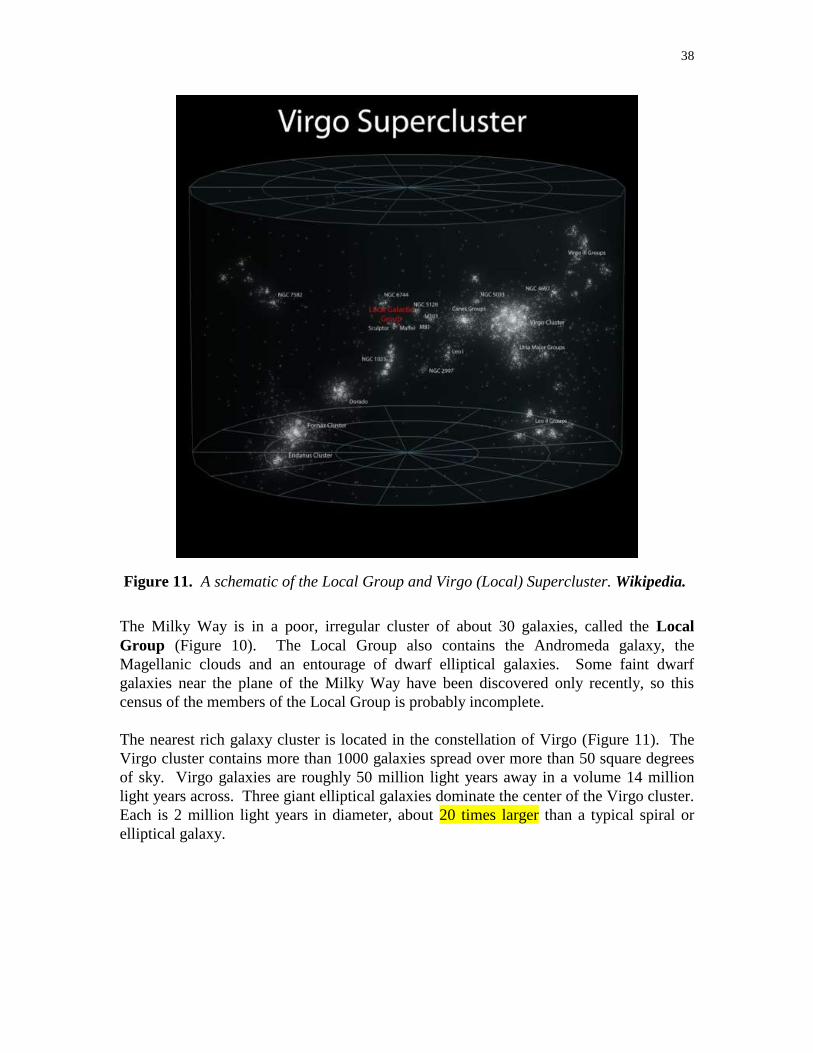
Figure 11. A schematic of the Local Group and Virgo (Local) Supercluster. Wikipedia.

The Milky Way is in a poor, irregular cluster of about 30 galaxies, called the Local

Group (Figure 10). The Local Group also contains the Andromeda galaxy, the

Magellanic clouds and an entourage of dwarf elliptical galaxies. Some faint dwarf

galaxies near the plane of the Milky Way have been discovered only recently, so this

census of the members of the Local Group is probably incomplete.

The nearest rich galaxy cluster is located in the constellation of Virgo (Figure 11). The

Virgo cluster contains more than 1000 galaxies spread over more than 50 square degrees

of sky. Virgo galaxies are roughly 50 million light years away in a volume 14 million

light years across. Three giant elliptical galaxies dominate the center of the Virgo cluster.

Each is 2 million light years in diameter, about 20 times larger than a typical spiral or

elliptical galaxy.

39

Figure 12. An image of the center of the Virgo cluster of galaxies showing two giant

elliptical galaxies. The Virgo cluster is the nearest rich cluster of galaxies to the Milky

Way. It contains hundreds of galaxies at a distance of about 50 million light years. FMW

541-27.4.

An example of a rich, regular galaxy cluster is the Coma cluster, some 300 million light

years away (Figure 13). Over 1000 Coma galaxies are visible, and possibly thousands of

dwarf ellipticals are not. Two giant elliptical galaxies are seen reigning in the center of

the Coma cluster.

Figure 13. The Coma cluster. APOD.

Way which prohibits us from seeing galaxies near the plane of our own galaxy. Notice the

clumps and voids in this distribution of galaxies. FMW 543-27.7.

Superclusters may contain dozens of clusters over a volume tens of millions of light-

years across (Figure 14). Superclusters are separated by gaps, typically spherical 100s of

millions of light-years in diameter. Galaxies appear concentrated on surfaces of spherical

40

bubbles. It is not know why galaxies appear to form on surfaces, but it is certainly a clue

to the conditions under which they formed, the conditions at the birth of the Universe.

Figure 14. The clustering and superclustering of galaxies on the sky. Wikipedia.

Summary

In the early part of this century it was thought that observed galaxies were located inside

the boundary of the Milky Way. With modern telescopes astronomers see billions of

galaxies filling the Universe, all outside of the Milky Way, each containing millions or

billions of individual stars. Galaxies can be classified according to their Hubble class as

spiral, elliptical, S0, irregular, or peculiar. Galaxies are clumped by gravity into clusters.

Our own galaxy is in the Local Group, an irregularly shaped cluster of about 30 galaxies,

41

including Andromeda and the Magellanic Clouds. Rich galaxy clusters can contain more

than 1000 galaxies. Even galaxy clusters are clumped into galaxy superclusters.

Key Words & Phrases

1. Elliptical galaxy – a spheroid galaxy with no spiral arms

2. Induction

3. Irregular cluster – a cluster of galaxies with an irregular and non-spherical

distribution of galaxies

4. Irregular galaxy – a usually small galaxy with an amorphous, irregular shape

5. Local Group – the galaxy cluster containing the Milky Way, Andromeda, the Large

Magellanic Cloud, the Small Magellanic Cloud, and approximately 30 other members

6. Peculiar galaxy – a galaxy that doesn’t fall cleanly into the other Hubble galaxy

classifications

7. Poor cluster – a galaxy cluster with a relatively small number of members

8. Rich cluster – a galaxy cluster with a large number of members

9. Regular cluster – a cluster of galaxies with a roughly spherical distribution

10. S0 galaxy – a galaxy that contains a disk of stars with a smooth distribution of stars

and no spiral arms

11. Spiral galaxy - a galaxy that contains a disk of stars exhibiting at least two spiral

arms

Review for Understanding

1. How do we know that other galaxies are indeed extragalactic?

2. How do astronomers classify galaxies? What are the characteristics of each major

type? Which type is most common?

3. How do galaxies cluster? What types of clusters of galaxies are there?

4. What are the brightest galaxies in the Local Group?

Essay Questions

1. How would we classify the Milky Way if it had formed all of its stars before it had a

chance to go through disk collapse? Why?

2. Why can’t galaxies evolve from elliptical to spiral or from spiral to elliptical on the

Hubble tuning fork diagram?

42

________________________________________________________________________

Chapter 23 – How Big is Our Universe? ________________________________________________________________________

The contemplation of things as they are, without error or confusion, without substitution

or imposture, is itself a nobler thing than a whole harvest of invention.

--Francis Bacon

In the space of one hundred and seventy-six years the Lower Mississippi has shortened

itself two hundred and forty-two miles. That is an average of a trifle over one mile and a

third per year. Therefore, any calm person, who is not blind or idiotic, can see that in the

old Oolitic Silurian Period, just a million years ago next November, the Lower

Mississippi River was upward of one million three hundred thousand miles long, and

stuck out over the Gulf of Mexico like a fishing-rod. And by the same token any person

can see that seven hundred and forty-two years from now the Lower Mississippi will be

only a mile and three-quarters long, and Cairo and New Orleans will have joined their

streets together, and be plodding comfortably along under a single mayor and a mutual

board of aldermen. There is something fascination about science. One gets such

wholesale returns of conjecture out of such trifling investment of fact.

--Mark Twain, Life on the Mississippi (1875)

Chapter Preview

In this chapter we will attempt to answer the question, “How big is our Universe?”

Measuring the distances to astronomical objects is one of the most difficult, mundane,

and surprisingly fruitful enterprises of the astronomer. It leads naturally to the discovery

of the answers to questions regarding the size of our Universe, and in the 20th

century has

surprised astronomers with measurements that tell us much more about our Universe. As

seen everywhere in the scientific enterprise, measurements that answer one question

usually lead to many more.

Key Physical Concepts to Understand: standard candle and standard meter stick

methods for distance determination, variable stars, and the Hubble relation

I. Introduction

One of the most fundamental yet difficult measurements in astronomy is the measurement

of the distance to a distant object. Without distance determinations we are only able to

view our Universe in two dimensions, as it appears projected onto the sky. In order to

construct a conceptual 3-dimensional model of our galaxy, our Local Group, the local

supercluster, or the Universe as a whole, it is essential that we are able to measure, or at

the very least estimate, the distances to stars and galaxies.

43

There are four basic types of techniques that are currently used to determine the distances

to astronomical objects: radar ranging, parallax, standard candle techniques, and

standard meter stick techniques. The first two are quite specific and are limited to

relatively nearby objects; the latter are categories that encompass a variety of related

methods.

I. Standard Candle Techniques

A standard candle technique is any distance measurement or estimation method that

depends on the inverse square law of light: objects of known luminosity have a

predictable brightness when they are placed at a given distance from an observer. This

method is one that people use at night when driving a car. If we see the headlights of an

oncoming car, we can estimate its distance by assuming that car headlights have a single

luminosity (Figure 1). This assumption is not strictly true, different headlights will have

different luminosities depending on their model, age, the voltage fed to them, and just

random headlight-to-headlight variations. However, most headlights have luminosities

within a certain range, and that range is small enough to allow us to make crude distance

estimations, good enough to allow us to determine whether or not it is safe to pass the car

in front of us. Judging distance from headlight brightness is just one example of a

standard candle technique.

Figure 1. Photo of cars on a freeway at night.

44

Mathematical Illustration of the Standard Candle Technique

Given two main sequence stars of the same spectral type: Star A is 10 light-years away.

Star B is at an unknown distance but appears 100 times fainter than Star A. How far

away is Star B?

The brightness of objects, whether they are candles, headlamps, or stars, falls with the

square of the distance (as given by the inverse square law of light, Chapter 5, Section VI).

Stated in the form of a mathematical equation:

Brightness = constant / Distance2

For Star A and Star B we may write:

Brightness of A = constant / (Distance of A)2 ,

and Brightness of B = constant / (Distance of B)2.

Dividing these two equations, we can determine the ratio of distances from the ratio of

brightnesses, or vice versa:

BA/BB = DB2/DA

2,

where BA and BB are the brightnesses of Stars A & B, and DA and DB are their distances.

In our case we know that BA is 100 times BB and that DA is 10 light years, so that:

100 = DB2 / (10 light years)

2, or rearranging, DB

2 = (10 light years)

2 x 100.

DB = square root((10 light years)2 x 100) = 100 light years.

The distance to Star B is 10 light years.

Table 25.1: Standard Candle Distance Determination Methods

Technique Range of Use

Spectroscopic Parallax 1 million parsecs

to edge of the Milky Way

Variable Stars 20 million parsecs

most distant stars in nearby galaxies

Supernovae 100s of millions of parsecs

to distant galaxies

Galaxy Luminosity 300 million parsecs

to distant galaxies

45

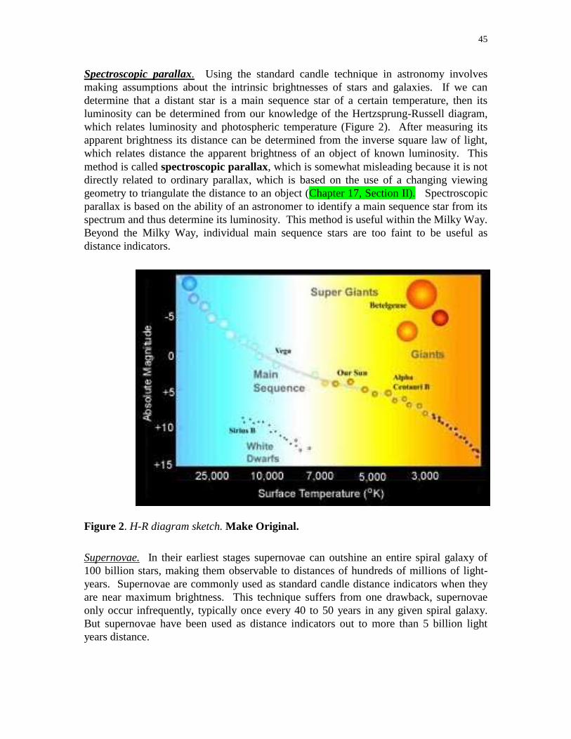
Spectroscopic parallax. Using the standard candle technique in astronomy involves

making assumptions about the intrinsic brightnesses of stars and galaxies. If we can

determine that a distant star is a main sequence star of a certain temperature, then its

luminosity can be determined from our knowledge of the Hertzsprung-Russell diagram,

which relates luminosity and photospheric temperature (Figure 2). After measuring its

apparent brightness its distance can be determined from the inverse square law of light,

which relates distance the apparent brightness of an object of known luminosity. This

method is called spectroscopic parallax, which is somewhat misleading because it is not

directly related to ordinary parallax, which is based on the use of a changing viewing

geometry to triangulate the distance to an object (Chapter 17, Section II). Spectroscopic

parallax is based on the ability of an astronomer to identify a main sequence star from its

spectrum and thus determine its luminosity. This method is useful within the Milky Way.

Beyond the Milky Way, individual main sequence stars are too faint to be useful as

distance indicators.

Figure 2. H-R diagram sketch. Make Original.

Supernovae. In their earliest stages supernovae can outshine an entire spiral galaxy of

100 billion stars, making them observable to distances of hundreds of millions of light-

years. Supernovae are commonly used as standard candle distance indicators when they

are near maximum brightness. This technique suffers from one drawback, supernovae

only occur infrequently, typically once every 40 to 50 years in any given spiral galaxy.

But supernovae have been used as distance indicators out to more than 5 billion light

years distance.

46

Sc Galaxies. Although galaxies as a whole vary widely in luminosity, individual galaxy

classes have a reasonably small luminosity variation. Elliptical galaxies and irregular

galaxies in particular have wide luminosity ranges. Sc galaxies are used in determining

the distance to distant galaxy clusters, where most other techniques lack sensitivity.

II. The Distance Determination Ladder

As shown in Figure 3, astronomical distance determination techniques form a distance

determination ladder. Each method depends on a method used for determining distances

to more nearby celestial objects. The Sun is 8 light minutes away. The next nearest star

is 4 light years distant. The most distant quasars are as far away as 13 billion light years.

We can’t use a single method for distance determination. Radar is the most precise

distance determination technique, but can only be used to find the distances to planets.

Knowing the distance from the Earth to the Sun, from radar ranging, we can determine

the distance to nearby stars from the use of parallax, the amount of apparent shift that is

seen for an object in the sky as the Earth orbits the Sun. In order to determine the

distance that an object has from its parallax, we must already know the size of the Earth’s

orbit. The size of the Earth’s orbit is calculated by measuring the distance between the

Earth and a number of other planets over a period of years.

Figure 3. The cosmic distance ladder. This chart shows a variety of methods of

measuring the distances to celestial objects and the distances over which these methods

are appropriate. The measurement errors, measured as a percentage, are larger for more

distant objects. P 563-31.34.

Once the parallax method has been calibrated it is in turn used to calibrate the method of

spectroscopic parallax. Distances are determined to nearby stars of known spectral type

using trigonometric parallax. After the luminosity of a number of stars of each spectral

47

type has been determined, they can be used as standard candles. Each of the distance

determination methods is useful over a limited range of distance. Larger and/or brighter

objects must be found for use as standard candles or standard meter sticks for larger

distances. Errors accumulate with each method used, so that by the time distance

determinations are being made to distant galaxies, the accumulated error can be quite

large. At great distances, in order to avoid the error associated with an individual

measurement it is often desirable to measure the distances to many galaxies in a single

cluster, all at the same red shift. Then all of the galaxies can be attributed the same

distance, the mean of all the measures.

III. Standard Meter Stick Techniques

A standard meter stick technique is any distance determination technique that uses the

apparent size of an object of known size to determine its distance. A meter stick held

perpendicular to the line of sight occupies an angle of 11 degrees at a distance of five

meters. When moved to a distance of 10 meters it will occupy an angle of only 5.5

Degrees. The angular size of an object decreases in proportion to its distance. (For

additional examples see Chapter 2, Section IV.) When driving we can and do estimate

the distance to cars and people by how large they appear. In doing this we assume that

cars and people come in reasonably standard sized packages. We also estimate the

distance to a faraway building by its apparent height and the distance to an intersection in

the highway by the apparent width of the highway at the point of intersection or the

distance to a stand of trees by the width of nearby railroad tracks (Figure 4). Any distance

determination/estimation technique is based on the assumption that objects of an

identifiable type (e.g. cars, people, and roads) come in identical or at least similar sizes.

Stars at any distance beyond the Sun are too small to use as standard meter sticks, but HII

regions, the giant gas clouds ionized by O and B stars, and galaxies themselves have been

used as standard meter sticks. Parallax is now a viable technique for the telescopic

measurement of distances out to 300 light-years. The European satellite Hipparchos,

named after the Greek astronomer Hipparchus, extended that distance by making parallax

measurements of 100,000 stars out a distance of 3000 light-years.

48

Figure 4. Standard meter stick sketch. Original.

Table 2.2: Standard Meter Stick Distance Determination Methods

Technique Range of Use

HII Region Diameter Nearby galaxies

Galaxy Diameter To distant galaxies

IV. Variable Stars

Two of the most accurate and most frequently used astronomical standard candles are the

Cepheid and RR Lyrae variable stars (Table 23.1). Both are stars in the post-main

sequence stages of evolution. After core fusion of hydrogen to helium, post main

sequence stars change in luminosity and temperature, resulting in a changing position on

the H-R diagram. During its post main sequence evolution a star’s adjustments in

49

pressure and temperature can result in its instability for a time interval, resulting in a

periodically varying luminosity over short periods of time, possibly days. Stars in a

region of the H-R diagram above the main sequence, called the instability strip, are

known to pulsate (Figures 5 and 6).

Figure 5. The instability strip, that shaded region in the HR diagram where stellar

instability is manifested by variable stars. From http://institute-of-brilliant-

failures.com/section3.htm

50

Table 23.1: Characteristics of Cepheid and RR Lyrae Variables

Cepheids RR Lyrae variables

Mass

(suns)

Luminosity

(suns)

100-10,000 100

Period 1-150 days 0.3-0.9 days

Low-mass stars, after their post-helium flash, undergo a luminosity and photospheric

temperature change that takes them through the lower end of the instability strip. These

stars become RR Lyrae variables, named after their prototype in the constellation Lyra.

RR Lyrae variables all pulsate with periods less than one day.

Figure 6. Variable star light curves. Variations in a Cepheid variable star (delta

Cepheus) and RR Lyrae. From spiff.rit.edu and

51

www.astro.sunysb.edu/metchev/PHY515/cepheidpl.html

High-mass stars undergo a luminosity and photospheric temperature change that takes

them through the upper end of the instability strip. These pulsating stars are called

Cepheid variables named after the first discovered of their class in the constellation

Cepheus. Their sharp increase and gradual decrease in brightness distinguish them as

Cepheid variables (Figure 6).

What causes the periodic pulsation of stars in the instability strip? Spectra of RR

Lyrae and Cepheid variables show a varying Doppler shift of their absorption lines

synchronized with their changing brightness. This indicates that these stars are expanding

and contracting, oscillating in size, brightness and photospheric temperature. The

atmosphere of these variable stars is analogous to a weight on a spring (Figure 7). A

mass hanging on a stationary spring has its weight balanced by the tension force produced

in the spring pulling in the direction opposing gravity. Gravity pulls down and the spring

pulls up. Consequently the weight doesn’t move. If we pluck the mass downward and

release it the spring goes into an oscillation, periodically moving up and down. When the

mass is on the lowest excursion of its travel, the tension of the spring exceeds gravity and

the mass is pulled upward. As the mass travels through its original position of stability,

the forces of gravity and spring tension are equal so there is no net force on the mass. But

it is now moving with a significant velocity upward, so that it just keeps on moving.

After it passes through the equilibrium position the gravitational force on the mass is

larger than the spring tension, so the mass decelerates. Finally at its maximum excursion

upward the mass has decelerated to a stop. But it can’t remain there, for the gravitational

force exceeds the force of spring tension. In this way the mass will oscillate until

frictional energy losses kill the oscillation.

Figure 7. Weight on a spring.

In a Cepheid or RR Lyrae variable there is a similar situation. Just substitute pressure for

spring tension. As a star evolves and becomes unstable, atmospheric layers can expand

and contract. Once this begins an oscillation may set in. As the atmosphere reaches its

maximum compression, the force from gas pressure exceeds gravity and the atmosphere

will expand. Once set into motion the atmosphere will expand beyond the point at which

gas pressure and gravity are balanced. The atmosphere will continue to expand and cool,

decelerating all the while. The atmosphere will decelerate until it stops, reaching its

maximum excursion outward, and its minimum temperature and luminosity. At this point

gravity exceeds the force of gas pressure and the star will begin to contract, heat, and gain

in luminosity. Pulsations can become so violent that the star sheds its outer layer.

A precise relationship between the period and luminosity of Cepheid variables was

discovered by Harvard astronomer Henrietta Leavitt for Cepheid variables in the Small

Magellanic cloud in 1912 (Figures 8 and 9). In 1924 Hubble used this work to determine

the distance to the Andromeda galaxy and ended the debate about whether galaxies were

internal or external to the Milky Way. Because Cepheid variables are roughly 10,000

52

times the luminosity of the Sun, they are used to find the distances to galaxies out to

millions of light years. Hubble then used this period-luminosity relationship for

determining the distances to more distant galaxies.

Figure 8. Cepheid variables. Hubble Space Telescope images of a Cepheid variable in

M100. This color image is a Hubble Telescope Image of M100. The insets show the

variation of a single Cepheid variable in M100 over a one-month period. HST.

53

Figure 9. Period-luminosity relationship for Cepheids and RR Lyrae stars. This enables

astronomers to determine distances to these starts by 1) measuring their period, 2) using

that to calculate their luminosity, and 3) using their measured apparent brightness to

determine their distance. From http://zebu.uoregon.edu/~soper/MilkyWay/cepheid.html

RR Lyrae stars are low-mass Population II stars commonly found in globular clusters.

RR Lyrae variables also have a period-luminosity law (Figure 9). Because they are much

fainter than Cepheid variables, with luminosities in the range of hundreds of solar

luminosities, they are not useful for determining distances to other galaxies. They are of

great use in determining the structure of our own galaxy. In 1915, Harlow Shapley used

directions to Milky Way globular clusters along with distances measured by this period-

luminosity relationship to model the three-dimensional distribution of globular clusters in

the Milky Way. He found that they form a spherical system 100,000 light years in

diameter centered on a point in Sagittarius (Chapter 21, Figure 5). He assumed that these

outlined the true extent of the volume of the Milky Way and found that the Sun is not at

the center of the galaxy.

V. The Hubble Relation

After Hubble determined that Andromeda and, by inference, other galaxies were outside

the Milky Way, V.M. Slipher of Lowell Observatory measured the velocities of 40

galaxies from the Doppler shifts of their absorption lines (Figure 10). These galaxies had

large red shifts indicating velocities up to 1,800 km/s away from the Milky Way; none

had blue shifted spectra, which would indicate velocities toward the Milky Way. In 1929

Hubble published a comparison of the velocities of these galaxies and their distance as

estimated from photometry of Cepheid variables found in them. A high degree of

correlation was found between distance and velocity; the red shift of a galaxy was found

to be proportional to its distance (Figure 11), except for variations at small distances

caused by local effects such as the motion of galaxies in the Local Group toward the

Milky Way and Andromeda. This relationship is called the Hubble law and can be

expressed as:

54

Equation 25.1: velocity = H distance,

where H is a constant of proportionality called the Hubble constant.

Figure 10. The change in the wavelength of a spectral line, Δλ, is the difference between

the wavelength measured when the object is moving and the wavelength measured if the

object were at rest. The bottom spectrum shown below is for hydrogen in the lab (where

the speed of the object is v=0). The top spectrum is a representation of hydrogen lines in

a galaxy that is moving at four tenths of the speed of light away from us. The lowest

wavelength violet line is shifted redward until it appears in the orange part of the

spectrum.

55

Figure 11. The Hubble relation from his original work. Upper Panel. On the left are

elliptical galaxies in four galaxy clusters shown to the same scale. On the right are

spectra of these galaxies showing their red shifts. A laboratory comparison spectrum is

shown above and below the spectrum of each galaxy. The H and K lines of ionized

calcium are seen in each galaxy spectrum; the yellow arrows show how far each set of

galaxy lines has been red shifted. The velocity of each galaxy is shown below its

spectrum. Its distance, in megaparsecs, is shown next to the image of each galaxy. Panel

B: The Hubble diagram galaxies including those shown in Panel A. From

http://outreach.atnf.csiro.au/education/senior/cosmicengine/hubble.html

56

How do we account for the Hubble law? It is obvious that it is not somehow due to the

random motions of galaxies or simply an effect of their gravitational attraction to one

another, for nearly all galaxies are found to be moving away from the Milky Way. This

relationship would not be expected to occur in a static, unchanging Universe, but could be

expected to occur in an expanding one, in which all of space and the galaxies contained in

it are moving apart. This leads to a large number of questions. If the Universe is

expanding and we see all galaxies moving away from the Milky Way, is the Milky

Way at the center of the Universe? Is there any confirming evidence for such an

expansion? What caused the expansion? We will study the theories of the Universe

that physicists and astronomers have put forth to explain the Hubble law in Chapter 26

and look at the evidence that supports or denies these theories.

Summary

There are four basic types of techniques that are currently used to determine the distances

to astronomical objects: radar ranging, parallax, standard candle techniques, and standard

meter stick techniques. The first two are limited to relatively nearby objects. A standard

candle technique is any distance measurement or estimation method that depends on the

inverse square law of light; objects of known luminosity have a predictable brightness

when they are placed at a given distance from an observer. Standard candle methods

include spectroscopic parallax, variable stars, supernovae, and galaxy luminosity. A

standard meter stick technique is any distance determination technique that uses the

apparent size of an object of known size to determine its distance. Standard meter stick

methods include HII region and galaxy diameter measurements.

Two of the most accurate standard candles are Cepheid and RR Lyrae variable stars.

Both are post main sequence stars in the instability strip of the H-R diagram. These stars

vary in brightness as their atmosphere alternately expands and contracts. Their use as

standard candles is predicated on the relationship between period and luminosity for each

type. By plotting the distance vs. red shift of forty galaxies Edwin Hubble determined

that the Universe must be expanding in such a way that the observed velocity of a galaxy

is proportional to its distance. This is the Hubble law.

Key Words & Phrases

1. Cepheid variable

2. Hubble constant – the constant of proportionality in the Hubble law

3. Hubble law – the law which says that the cosmological expansion velocity of a

galaxy is proportional to its distance

4. Instability strip – the region on the H-R diagram which is occupied by variable stars

5. Standard candle technique – any astronomical distance determination technique

based on the inverse square law of light

57

6. Standard meter stick technique – any astronomical distance determination

technique based on the concept that the apparent size of an object is inversely

proportional to its distance

7. Spectroscopic parallax – the method of astronomical distance determination based

on the use of spectroscopic classification of a star to infer its luminosity, followed by

using its measured brightness to determine its distance

Review for Understanding

1. How do we interpret the red shifts of galaxies? What does it tell us?

Essay Questions

1.

58

_______________________________________________________________________

Chapter 24 – Active Galaxies: the Energy Problem _______________________________________________________________________

The real voyage of discovery lies not in seeking new landscapes but in having new eyes.

--Marcel Proust

The sciences do not try to explain, they hardly even try to interpret, they mainly make

models. By a model is meant a mathematical construct which, with the addition of certain

verbal interpretations, describes observed phenomena. The justification of such a

mathematical construct is solely and precisely that it is expected to work.

--John von Neumann

Chapter Preview

It takes one billion years for light to travel from a galaxy one billion light years distant to

the Earth. By photographing a galaxy at a distance of one billion light years we obtain a

picture of it as it was one billion years ago, not as it is now. As we look farther and

farther out into space we look further back in time. By taking snap-shots of galaxies at

increasing distances we can look at the evolutionary paths that galaxies have taken over

time, not for any individual galaxy, but for galaxies in general. When we do this we see

that in epochs past galaxies were not the same as they are now, but were significantly

more luminous. Some exhibited violently explosive events in their nuclei, so energetic

that they nearly defy explanation. In this chapter we will examine these active galaxies

and review the current theories of their central energy sources.

Key Physical Concepts to Understand: non-thermal emission of radiation, properties

of radio galaxies, Seyfert galaxies, BL Lacertae objects, and quasars, determination of

the maximum size of a radiation source from its variability, models of the energy

source(s) for active galaxies

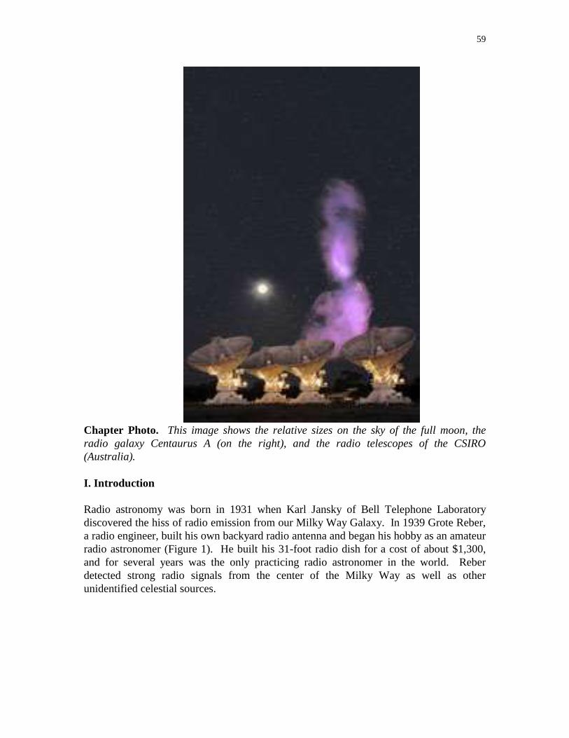
59

Chapter Photo. This image shows the relative sizes on the sky of the full moon, the

radio galaxy Centaurus A (on the right), and the radio telescopes of the CSIRO

(Australia).

I. Introduction

Radio astronomy was born in 1931 when Karl Jansky of Bell Telephone Laboratory

discovered the hiss of radio emission from our Milky Way Galaxy. In 1939 Grote Reber,

a radio engineer, built his own backyard radio antenna and began his hobby as an amateur

radio astronomer (Figure 1). He built his 31-foot radio dish for a cost of about $1,300,

and for several years was the only practicing radio astronomer in the world. Reber

detected strong radio signals from the center of the Milky Way as well as other

unidentified celestial sources.

60

Figure 1. Photo of Grote Reber’s radio telescope, in his backyard in Wheaton, IL.

Early radio astronomy began to flourish in England and Australia shortly after World War

II. Hundreds of radio sources were discovered, many of which were found to correspond

to optically visible counterparts. Some were associated with supernova remnants and

peculiar galaxies. Some radio-emitting galaxies manifested evidence of explosive

violence, such as extremely high luminosities and the ejection of large masses of gas at

high velocity (Figure 2). It was previously thought that galaxies were basically

quiescent, although every one hundred years or so an individual star in a galaxy might

supernova, as a collection of billions of stars, a galaxy would remain unchanged for

billions of years. With the era of radio astronomy began discoveries of galaxy luminosity

variability over short time periods, violent events in galaxy nuclei, and galaxies of

implausibly high luminosities. We call these active galaxies. The discovery of active

galaxies ushered in a new era of extragalactic research.

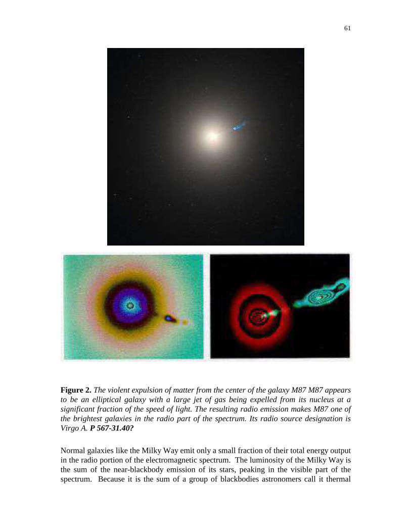
61

Figure 2. The violent expulsion of matter from the center of the galaxy M87 M87 appears

to be an elliptical galaxy with a large jet of gas being expelled from its nucleus at a

significant fraction of the speed of light. The resulting radio emission makes M87 one of

the brightest galaxies in the radio part of the spectrum. Its radio source designation is

Virgo A. P 567-31.40?

Normal galaxies like the Milky Way emit only a small fraction of their total energy output

in the radio portion of the electromagnetic spectrum. The luminosity of the Milky Way is

the sum of the near-blackbody emission of its stars, peaking in the visible part of the

spectrum. Because it is the sum of a group of blackbodies astronomers call it thermal

62

emission (Figure 3). Emission that does not approximate a blackbody or a group of

blackbodies is called non-thermal emission. Radio-emitting active galaxies are mostly

non-thermal in their electromagnetic spectra, with a brightness that remains constant or

even increases towards longer wavelengths (Figure 3). Non-thermal emission is usually

associated with the radiation from fast electrons gripped in spiral trajectories by a strong

magnetic field (Figure 4). This emission is called synchrotron emission because it is

observed in high energy particle accelerators of the same name. Synchrotron emission

occurs near the Earth’s magnetic poles in aurorae when solar particles spiral along the

Earth’s magnetic field. High luminosity non-thermal emission is a signature

characteristic of active galaxies.

Figure 3. Non-thermal (non-blackbody) emission from a quasar has a distinctly different

spectrum from thermal (blackbody) emission. Shown are two spectra, one a

representation of the type of emission that one would see from a quasar exhibiting

emission from high energy electrons moving through a magnetic field (synchrotron

emission, as seen in Figure 4), the other blackbody emission, an approximation of what

one would expect from a star. Attribution?

63

Figure 4. Electrons spiraling around lines of magnetic force give rise to the synchrotron

emission of electromagnetic radiation. P 523-30.6.

Let’s imagine a cube 300 million light-years on a side, centered on the Milky Way

(Figure 5). Inside the imaginary 300 million light-year cube galaxies are usually normal

spiral and elliptical galaxies with thermal emission spectra. However, outside this cube

we see many galaxies that do not fit this profile because they are active galaxies; they are

highly luminous, their luminosity varies with a time-scale of days to years, and they

exhibit a non-thermal emission spectrum with unusually strong radio emission. Many of

these active galaxies exhibit most of their luminosity from an almost unbelievably small

central region. Active galaxies are commonly classified into a number of groups

according to their characteristics: radio galaxies, Seyfert galaxies, BL Lacertae objects,

and quasars.

How are the distances to these galaxies determined? It is generally assumed that the

measured red shifts of galaxies are a result of the expansion of the Universe; their

distances are determined from their measured red shifts and the Hubble relation. In the

next three sections we will look sequentially at nearby active galaxies, moderate distance

active galaxies, and distant active galaxies.

II. Nearby Radio Galaxies

The Milky Way, like any normal (non-active) galaxy is radio quiet. Its thermal emission

peaks in the visible and decreases steadily toward longer wavelengths. As a result it

emits only roughly 0.1% of its luminosity in the radio portion of the spectrum. Nearby

radio loud galaxies can be divided into two types: core-halo radio galaxies and double-

lobed radio galaxies.

64

A. Core-Halo Radio Galaxy

Core-halo galaxies are elliptical in shape with emission from a small central core, perhaps

1 light year across. The core has a luminosity as high as 1050

ergs/s, a million times

greater than the total luminosity of the Milky Way. Weak radio emission can often be

detected from the 100,000 light year diameter halo, roughly the size of the Milky Way.

Most core-halo galaxies are faint in the visible portion of the spectrum.

M87 is a typical core-halo galaxy only 50 million light years distant (Figure 2). M87

would be classified as an elliptical galaxy but for a thin jet of gas emanating from its core;

as a result it is classified as a peculiar galaxy. M87 is roughly 100,000 light years across,

as is the Milky Way. The gas jet is 5,000 light years long travelling at 25,000 km/s

(nearly one-tenth the speed of light) as measured from the Doppler shift of the emission

lines originating in the gas.

Characteristics of Core-halo galaxies include:

A small non-thermal core (less than several light years across)

Highly luminous non-thermal emission ( a million times the luminosity of the Milky

Way)

Often associated with weak elliptical galaxies

High velocity ejection of gas from the nucleus (up to a significant fraction of the

speed of light.)

B. Double-Lobed Radio Galaxy

A typical example of a double-lobed radio galaxy is Centaurus A, an elliptical galaxy 15

million light years distant (Figure 5). Centaurus A is 100,000 light years across and

would be classified as an elliptical galaxy if not for the chaotic dust lane that bisects it;

the dust may have resulted from an explosion in its nucleus. As a result it is classified as

a peculiar galaxy. Radio emission is only weakly detected from the optical counterpart of

this galaxy. Most all of the radio emission occurs from its extended lobes. Each lobe is

about 400,000 light years across, much bigger than a typical galaxy. If a line were drawn

connecting the two lobes, the visible galaxy would be precisely in line with the radio

lobes and halfway between them. Centaurus A is 3 million light years across from end to

end, as large as our Local Group of galaxies is. Some double-lobed radio galaxies are

even larger, up to 10 million light years end-to-end (Figure 6), representing the largest

single galaxies observed. A second smaller and weaker set of lobes, each 50,000 light-

years in diameter, is seen interior to the large lobes in Centaurus A.

Characteristics of double-lobed radio galaxies:

No core radiation in the radio (an optical counterpart is often seen precisely midway

between the radio lobes).

The galaxies are enormous. (The lobes are up to 10 million light years across.)

Luminosities up to 1052

ergs/s (100 million times the luminosity of the Milky Way),

almost all in the radio.

65

Figure 5. The double-lobed radio Galaxy Centaurus A. Panel A: In visible light. Panel

B: near infrared, showing a galaxy that Cen A absorbed a half-billion years ago. Panel

C: A far infrared image, showing thermal emission from dust. Panel D: radio emission

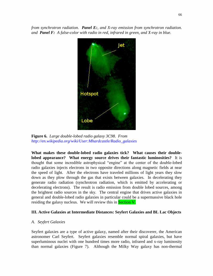
66

from synchrotron radiation. Panel E:, and X-ray emission from synchrotron radiation.

and Panel F: A false-color with radio in red, infrared in green, and X-ray in blue.

Figure 6. Large double-lobed radio galaxy 3C98. From

http://en.wikipedia.org/wiki/User:Mhardcastle/Radio_galaxies

What makes these double-lobed radio galaxies tick? What causes their double-

lobed appearance? What energy source drives their fantastic luminosities? It is

thought that some incredible astrophysical “engine” at the center of the double-lobed

radio galaxies injects electrons in two opposite directions along magnetic fields at near

the speed of light. After the electrons have traveled millions of light years they slow

down as they plow through the gas that exists between galaxies. In decelerating they

generate radio radiation (synchrotron radiation, which is emitted by accelerating or

decelerating electrons). The result is radio emission from double lobed sources, among

the brightest radio sources in the sky. The central engine that drives active galaxies in

general and double-lobed radio galaxies in particular could be a supermassive black hole

residing the galaxy nucleus. We will review this in Section V.

III. Active Galaxies at Intermediate Distances: Seyfert Galaxies and BL Lac Objects

A. Seyfert Galaxies

Seyfert galaxies are a type of active galaxy, named after their discoverer, the American

astronomer Carl Seyfert. Seyfert galaxies resemble normal spiral galaxies, but have

superluminous nuclei with one hundred times more radio, infrared and x-ray luminosity

than normal galaxies (Figure 7). Although the Milky Way galaxy has non-thermal

67

emission originating in its nucleus, it is only a small fraction of its total energy output,

roughly 0.1%. With a core luminosity of 1046

ergs/s, Seyfert nuclei can be a million

times more luminous than the center of our own galaxy. Doppler velocity measurements

from spectroscopy of Seyfert nuclei reveal clouds of hot gas ejected at high velocities,

1,000 km/s. This gas has similar emission lines as the center of the Milky Way. The

Seyfert galaxy phenomenon may represent a few percent of all spiral galaxies. Seyfert

nuclei are variable, the luminosity changing by a factor of 2 within a year. High-

resolution radio maps confirm that this variability originates from an incredibly small

region at the galaxy center, not much larger than the Oort comet cloud surrounding our

Solar System. Astronomers suspect that violent explosions are the culprits that cause

Seyfert nuclei variability, high-intensity bursts of energy emanating from the compact

nucleus. Similar events are seen in the Milky Way, but Seyfert events are literally one

million times more dramatic.

Characteristics of Seyfert galaxies:

3-5 billion light years distant

a typical spiral with an active nucleus.

nuclear gases moving at 1,000 km/sec

a nucleus one million times brighter than the Milky Way nucleus, 100 times brighter

than the entire Milky Way

radio and infrared radiation is strong, as is X-ray emission

variable on a time scale of a year

Is a Seyfert galaxy a phase in every spiral galaxy’s evolution or a classification of a

small percentage of galaxies? Seyfert galaxies represent 2-5% of all galaxies seen at

near to moderate distances. Does this mean that only a small percentage of all spiral

galaxies go through this phase? No. When shopping at the mall you might notice that

only a small percentage of women are obviously pregnant. This does not mean that only

a small percentage of women ever bear children, it just means that the latter stages of

pregnancy are short compared to the mean lifetime of a woman. The Seyfert galaxy

phase might be a relatively short phase in the life of a spiral galaxy when its nucleus

becomes extremely active. The same principle may apply to all types of active galaxies.

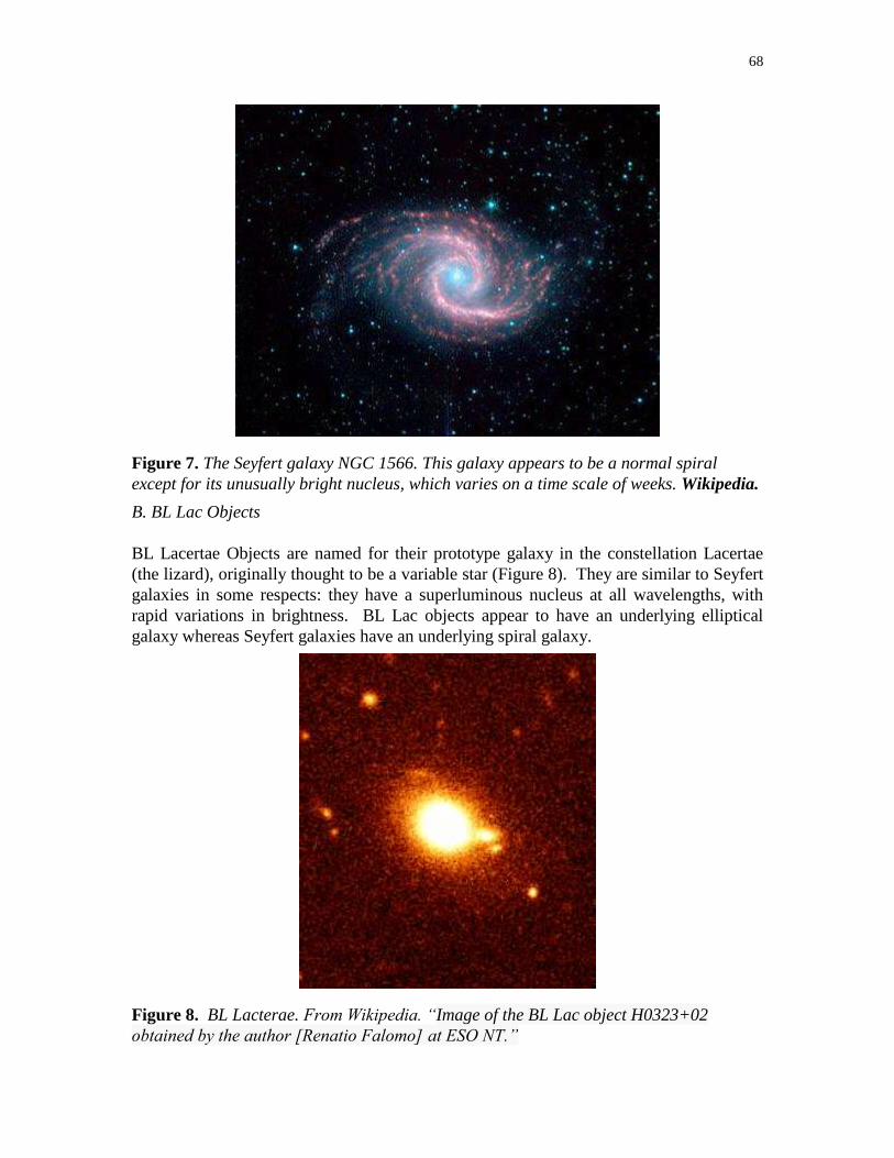
68

Figure 7. The Seyfert galaxy NGC 1566. This galaxy appears to be a normal spiral

except for its unusually bright nucleus, which varies on a time scale of weeks. Wikipedia.

B. BL Lac Objects

BL Lacertae Objects are named for their prototype galaxy in the constellation Lacertae

(the lizard), originally thought to be a variable star (Figure 8). They are similar to Seyfert

galaxies in some respects: they have a superluminous nucleus at all wavelengths, with

rapid variations in brightness. BL Lac objects appear to have an underlying elliptical

galaxy whereas Seyfert galaxies have an underlying spiral galaxy.

Figure 8. BL Lacterae. From Wikipedia. “Image of the BL Lac object H0323+02

obtained by the author [Renatio Falomo] at ESO NT.”

69

IV. Quasi-Stellar Radio Sources

In the 1960s dozens of radio sources were identified with optical galaxies; many were

associated with elliptical galaxies. One of these was 3C 48, the 48th

radio source in the

3rd

Cambridge catalog of radio sources. 3C 48 didn’t look extended like a galaxy but

appeared point-like, as a star. Many astronomers thought that it was a radio-emitting star.

Other radio sources were also discovered that were later identified with objects that

appeared to be unusually blue, faint stars on visible wavelength photographs. These were

later called quasi-stellar radio sources, or quasars for short (Figure 9). Optical

spectroscopy revealed emission lines at wavelengths that did not correspond to known

atoms. In 1963, Martin Schmidt of Mount Wilson studied four emission lines in a radio

source called 3C 273. He found these lines made physical sense if he assumed that they

came from four hydrogen lines red shifted at 14.5% of the speed of light. Now all

quasars can be explained as emission from gas of ordinary composition at unusually high

velocities, some at more than 90% of the speed of light. It was discovered that not all

high red shifted point-like galaxies are radio sources, but the name stuck. All high red

shift quasi-stellar galaxies are now called quasars, radio loud or not. There are currently

approximately 8,000 galaxies classified as quasars, approximately one out of every 1,000

galaxies. Again, the question is “Is a quasar a short phase through which every

galaxy passes, or is it a rare type of galaxy?”

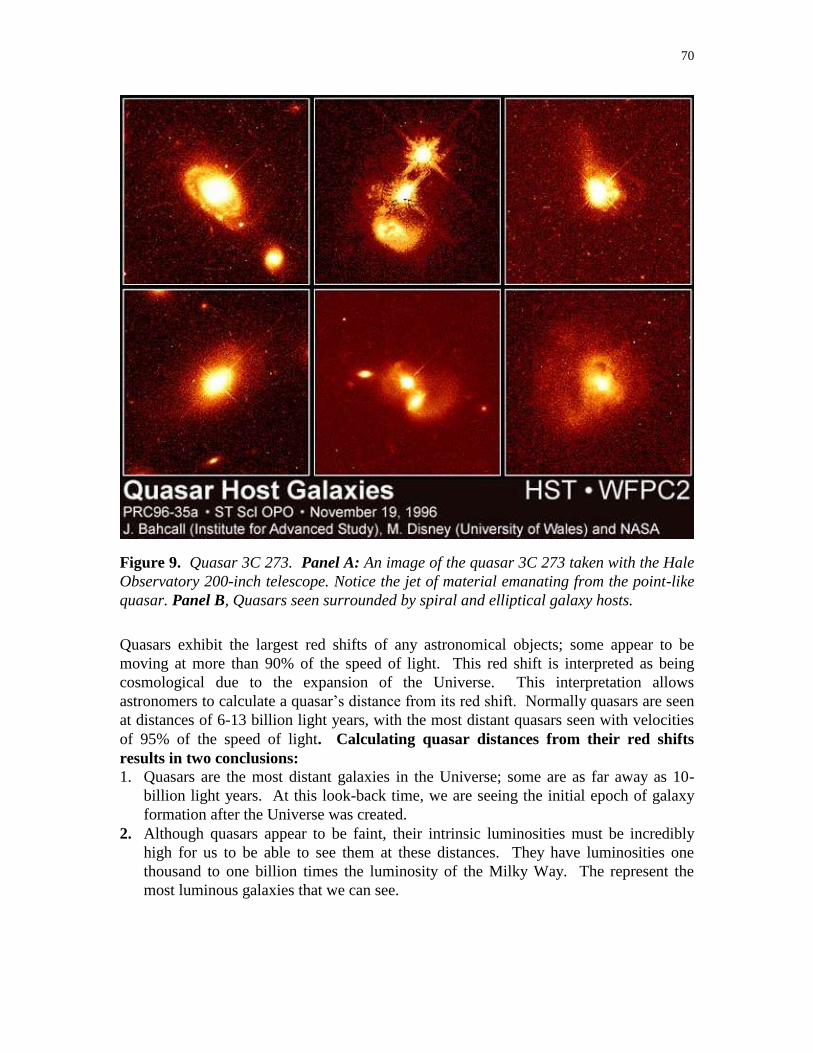
70

Figure 9. Quasar 3C 273. Panel A: An image of the quasar 3C 273 taken with the Hale

Observatory 200-inch telescope. Notice the jet of material emanating from the point-like

quasar. Panel B, Quasars seen surrounded by spiral and elliptical galaxy hosts.

Quasars exhibit the largest red shifts of any astronomical objects; some appear to be

moving at more than 90% of the speed of light. This red shift is interpreted as being

cosmological due to the expansion of the Universe. This interpretation allows

astronomers to calculate a quasar’s distance from its red shift. Normally quasars are seen

at distances of 6-13 billion light years, with the most distant quasars seen with velocities

of 95% of the speed of light. Calculating quasar distances from their red shifts

results in two conclusions:

1. Quasars are the most distant galaxies in the Universe; some are as far away as 10-

billion light years. At this look-back time, we are seeing the initial epoch of galaxy

formation after the Universe was created.

2. Although quasars appear to be faint, their intrinsic luminosities must be incredibly

high for us to be able to see them at these distances. They have luminosities one

thousand to one billion times the luminosity of the Milky Way. The represent the

most luminous galaxies that we can see.

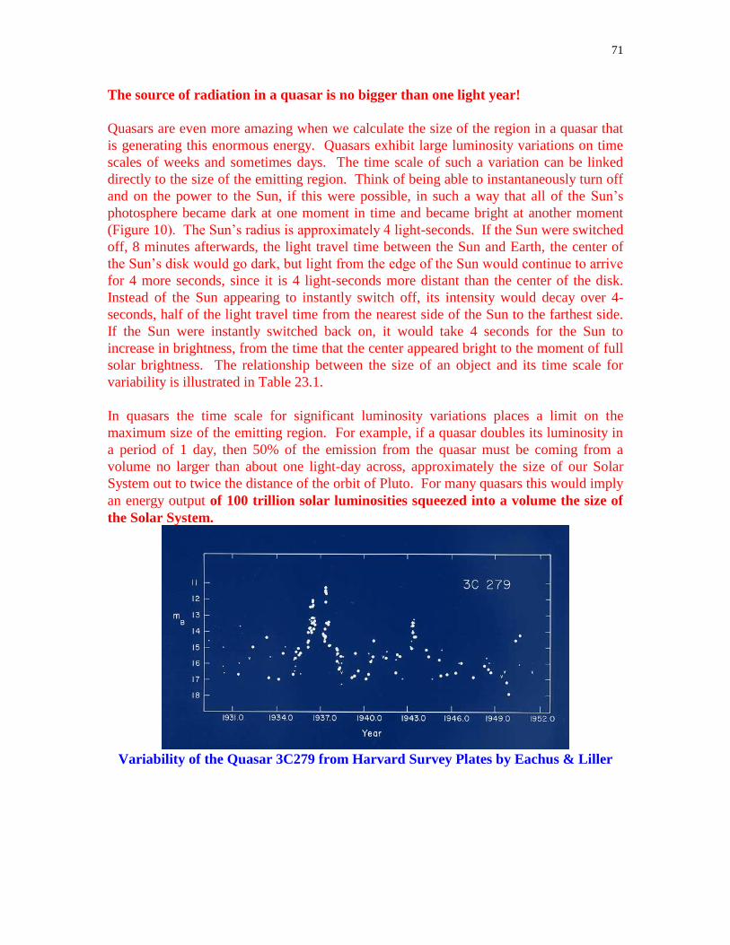
71

The source of radiation in a quasar is no bigger than one light year!

Quasars are even more amazing when we calculate the size of the region in a quasar that

is generating this enormous energy. Quasars exhibit large luminosity variations on time

scales of weeks and sometimes days. The time scale of such a variation can be linked

directly to the size of the emitting region. Think of being able to instantaneously turn off

and on the power to the Sun, if this were possible, in such a way that all of the Sun’s

photosphere became dark at one moment in time and became bright at another moment

(Figure 10). The Sun’s radius is approximately 4 light-seconds. If the Sun were switched

off, 8 minutes afterwards, the light travel time between the Sun and Earth, the center of

the Sun’s disk would go dark, but light from the edge of the Sun would continue to arrive

for 4 more seconds, since it is 4 light-seconds more distant than the center of the disk.

Instead of the Sun appearing to instantly switch off, its intensity would decay over 4-

seconds, half of the light travel time from the nearest side of the Sun to the farthest side.

If the Sun were instantly switched back on, it would take 4 seconds for the Sun to

increase in brightness, from the time that the center appeared bright to the moment of full

solar brightness. The relationship between the size of an object and its time scale for

variability is illustrated in Table 23.1.

In quasars the time scale for significant luminosity variations places a limit on the

maximum size of the emitting region. For example, if a quasar doubles its luminosity in

a period of 1 day, then 50% of the emission from the quasar must be coming from a

volume no larger than about one light-day across, approximately the size of our Solar

System out to twice the distance of the orbit of Pluto. For many quasars this would imply

an energy output of 100 trillion solar luminosities squeezed into a volume the size of

the Solar System.

Variability of the Quasar 3C279 from Harvard Survey Plates by Eachus & Liller

72

Figure 10. Variability of quasars relates to the size of the energy source. If a 1-light week

radius source and a 1 light-year radius source are turned on abruptly, it takes 1 week for

the small object to appear to come up to full intensity and 1 year for the larger object.

Similarly, if both are turned off abruptly, the larger object experiences 1 year of

decreasing intensity, the smaller object 1 week. From

http://casswww.ucsd.edu/archive/public/tutorial/Quasars.html

Table 23.1: Estimating the Size of an Object from its Variability Time Scale

Variability Time Scale

Maximum Size of

Emitting Region (km)

Object of

Similar Size

0.01 seconds 3000 Moon

1 second 3.0 105 Moon’s Orbit

5 seconds 1.5 106 Sun

8.3 minutes 1.5 108 Earth’s Orbit

1 hour 1.8 109 Jupiter’s Orbit

1 day 2.6 1010

1 week 1.8 1011

1 year 9.5 1012

Oort comet cloud

73

Figure 11. Gravitational lensing of a quasar. This peculiar object, called an Einstein

cross, provides verification of the General Theory of Relativity and the great distance of

quasars. The four bright objects are actually four copies of a single quasar, 8 billion

light years away, lensed by the surrounding fuzz, a foreground elliptical galaxy at a

distance of 400 million light years. FMW 532-26.20a? APOD.

In the years after the discovery of quasars, astronomers were not entirely happy with the

idea that there were galaxies whose energy sources were a billion times more luminous

than the whole of the Milky Way. After all, there were no satisfactory models for this

luminosity. Alternative models were suggested that placed quasars nearby, in the

neighborhood of the Milky Way. This would make it easy to explain their apparent

brightness. One suggestion had them as objects being ejected from the nucleus of our

Milky Way. Another attributed their enormous red shifts as gravitational red shifts of

local objects. Observations in the last ten years have proved beyond a shadow of a doubt

that quasars are not local objects, and in fact are at the distances suggested by their red

shifts. This evidence includes gravitational lensing, a general relativistic effect, of a

quasar by a more nearby galaxy, resulting in multiple images of the quasar (Figure 11)

and the detection of faint galaxies in the same cluster as “normal” galaxies, all at the

same red-shift. High sensitivity images of quasars in many cases show an extended

nebulosity, reminiscent of the outer portion of a typical faint galaxy.

One of the most distant quasars is the radio source 3C275.1, with a red shift

corresponding to a distance of 7 billion light years. Figure 12 shows that this quasar is

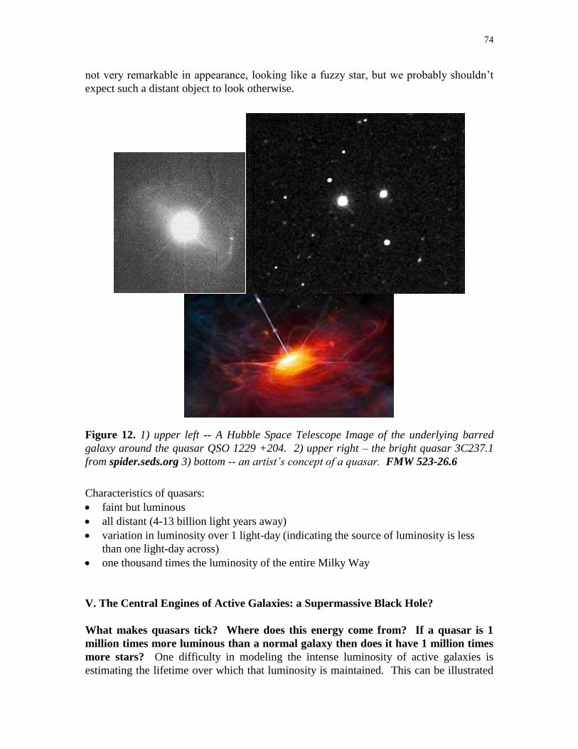
74

not very remarkable in appearance, looking like a fuzzy star, but we probably shouldn’t

expect such a distant object to look otherwise.

Figure 12. 1) upper left -- A Hubble Space Telescope Image of the underlying barred

galaxy around the quasar QSO 1229 +204. 2) upper right – the bright quasar 3C237.1

from spider.seds.org 3) bottom -- an artist’s concept of a quasar. FMW 523-26.6

Characteristics of quasars:

faint but luminous

all distant (4-13 billion light years away)

variation in luminosity over 1 light-day (indicating the source of luminosity is less

than one light-day across)

one thousand times the luminosity of the entire Milky Way

V. The Central Engines of Active Galaxies: a Supermassive Black Hole?

What makes quasars tick? Where does this energy come from? If a quasar is 1

million times more luminous than a normal galaxy then does it have 1 million times

more stars? One difficulty in modeling the intense luminosity of active galaxies is

estimating the lifetime over which that luminosity is maintained. This can be illustrated

75

by using a supernova as an example. A supernova with a peak luminosity of 1044

ergs/sec

can outshine an entire galaxy for a time scale of a year or so (roughly 107 seconds). But

its total energy output is equal to its luminosity (the amount of energy radiated per unit

time) times its lifetime. A supernova has a very intense, but very short lifetime. Using

equation 23.1 one can calculate the total amount of energy that it will radiate:

1044

ergs x 107 seconds = 10

51 ergs. This is only about ten times the amount of energy

radiated by the Sun over its lifetime, because the Sun will have a much greater longevity

than a supernova.

A high luminosity quasar has an energy output of 1052

ergs/s. To power it with

conventional one solar mass stars would require 1019

stars, equivalent to 100 billion

Milky Way galaxies, all packed into a region the size of the Solar System. No objects in

the Universe with anywhere close to this mass range are thought to exist. Stars are not

the most efficient way of generating energy since only 0.7% of the mass of hydrogen is

converted to energy when it fuses into helium, and only the inner ~10% of a one solar

mass star fuses hydrogen, for an overall efficiency of less than 0.1%. But the Sun

produces energy for 10 billion years. We don’t really know how long an active galaxy

remains active. We must compare the total amount of energy generated by stars like the

Sun with the total amount of energy expected to be generated over the lifetime of an

active galaxy. This total energy is given by equation 23.1. Comparisons of the total

energy output of the Sun, a 1 megaton nuclear bomb, and the Milky Way are given below:

Equation 23.1: Energy = Luminosity Lifetime

Nuclear Explosion (1 megaton)

Luminosity = 1023

ergs/sec

10-6

sec duration

= 1017

ergs (for comparison 107 ergs/sec = 1 watt)

Sun

Luminosity = 1033

ergs/sec

1017

sec lifetime

= 1050

ergs

Milky Way

Luminosity = 1011

stars 1033

ergs/sec/star = 1044

ergs/sec

1017

sec lifetime

= 1061

ergs

\

76

Table 23.1: Energy Output of Normal & Active Galaxies

Object Luminosity

(ergs/s)

Total Energy Over

Object’s Lifetime (ergs)

Nuclear Bomb 1023

1017

Sun 1033

1050

Supernova 1048

1054

Galactic Center 1040

1057

Milky Way Galaxy 1044

1062

Luminous Galaxy 1045

1063

Seyfert Galaxy 1046

unknown

Radio Galaxy 1046

-1052

unknown

Quasar 1046

-1053

unknown

Black hole candidates have been found at the centers of the nearby galaxies M31

(Andromeda), M32, M104, and M87, as well as our own Milky Way. Spectroscopic red

shift measurements of the core of M31, for example, show that stars within 50 light years

of the center are orbiting at speeds which from Kepler’s 3rd

law indicate 50 million solar

masses inside this radius (Figure 13). Such a large mass density would suggest the

presence of a supermassive black hole.

Figure 13. X-ray emission from a black hole accretion disk (bright blue in the X-ray

image) at the center of M31. NASA.

77

Recent Hubble Space Telescope images show M87 (Figure 14) to be a double-lobed

elliptical galaxy with a bright disk at its center, trailing spiral arms of matter from an

exceptionally bright nucleus. From Doppler measurements of material orbiting the

nucleus of M87 it appears the nucleus is dominated by a 6.6 billion solar mass black hole

and its accretion disk.

It is not unexpected that supermassive black holes would be common at the centers of

galaxy nuclei. Although no one has indisputably identified even a single nearby black

hole, evidence for their existence is strong (Chapter 20, Section IV). And while a 10

solar mass black hole is unbelievable dense: 1014

g/cm3, the densities of black holes drop

with increasing mass. A 1 billion solar mass black hole would only have a density of 2%

of that of water. Moreover it is logical to expect that during the collapse of a galaxy-

forming cloud of gas and dust an enormous amount of matter would eventually gravitate

(literally) to the center of mass of a galaxy, eventually achieving a high enough density to

form a supermassive black hole.

Figure 14. Evidence of a black hole at the center of the galaxy M87. To the left are

Doppler-shifted emission lines from the opposite sides of the disk at the core of M87. The

large Doppler shifts indicate that a disk of dust and gas is rotating at a velocity of 550

km/s, indicating that gas is orbiting a supermassive object. FMW 527-26.13.

Black holes, if common at galaxy centers, could explain active galaxies. As in accretion

disks around lower mass black holes (Chapter 20, Section IV), infalling matter is

78

expected to form a bottleneck near the black hole event horizon, forming a spinning disk

of dust and gas (Figure 15). As matter spirals towards the black hole its density increases.

The orbital velocity of matter increases as one approaches the event horizon. Friction

occurs between particles as they collide with each other at high velocity. This friction

heats the accretion disk, which radiates energy throughout the electromagnetic spectrum.

This conversion of gravitational potential energy to light is much more efficient than the

production of energy by nuclear fusion. The luminosity produced by infalling mass

converted to energy can account for the luminosity of a quasar with only about 30

solar masses of infalling material per year.

Figure 15. A painting of a black hole and its accretion disk, with two beams of matter

being ejected from a region just outside the Schwarzschild radius. FMW 530-26.16.

Not all of the infalling matter would move through the event horizon. Ultra-high

temperatures in the inner part of the accretion disk create an intense pressure that sends an

expanding gas through the only path that is not blocked by infalling matter, up through

the poles of the accretion disk, forming opposite jets of high velocity particles. Similar to

the pulsar model, two beams of accelerating particles are expelled that will produce

intense synchrotron radiation when they are slowed.

Why is matter ejected in narrow jets? It is thought that ejected mass is forced into

narrow beams by the infalling material which spirals into the black hole in an accretion

disk. The expelled material might also be focused by a magnetic field, so that charged

particles follow the polar magnetic field lines, as has been modeled for pulsars (Chapter

19, Section VI).

79

What evidence is there of an accretion disk in a galaxy nucleus? Hubble Space

Telescope images of galaxy nuclei show evidence of intense central emission in M51 as

well as the galaxies M32, M87, and M104, mentioned above. M51 (Figure 16) shows an

edge-on dust disk that bisects lobes of visible and radio emission. The disk is seen to be

about 100 light years in diameter.

Figure 16. Hubble image of the core of M51, with the X marking the central black hole

and the thick bar in the X indicating an accretion disk. NASA.

How can the supermassive black hole accretion disk explain active galaxies? Nearby

radio galaxies are seen either as double-lobed sources or core-halo sources. The

difference might simply be an effect of viewing geometry. A radio source seen with its

accretion disk edge-on would exhibit two lobes of radiation from the material exiting the

twin poles of the supermassive black hole (Figure 17). A radio source seen face-on

would appear as a core-halo source as we would view only the end of a single high-

energy jet.

80

Figure 17. Unification by viewing angle. From bottom to top:down the jet - Blazar, at an

angle to the jet -Quasar/Seyfert 1 Galaxy, at 90 degrees from the jet - Radio

galaxy / Seyfert 2 Galaxy[13]

What about Seyfert galaxies, BL Lac Objects, and quasars? The difference

between active galaxies of different types may be evolutionary. Quasars are seen only

at great distances, Seyfert galaxies and BL Lac Objects are seen primarily at intermediate

distances, and “normal” galaxies and radio galaxies dominate space within several

hundred million light years. This would seem to indicate that in the initial epoch of

galaxy formation, galaxy nuclei looked like quasars, perhaps due to the infall of relatively

large amounts of material into galaxies’ central black hole. The net result was a super-

luminous core. As galaxies evolved over billions of years this infall rate would be

expected to level off and slow down, producing less luminous cores. When the core is

seen at the center of a spiral galaxy we might have a Seyfert galaxy, when seen at the

center of an underlying elliptical galaxy we might have a BL Lacertae object. When

galaxies continue to evolve and the black hole mass infall rate continues to decline we

might expect to see active galaxy cores of more limited luminosities, ordinary radio

galaxies and typical galaxies like the Milky Way. This scenario is a popular but

speculative hand-waving model of active galaxies. Real physical models await more data

and much more computer modeling by theorists.

81

WebVideo: The Active Galaxy Seen from Different Points of View

http://www.youtube.com/watch?v=6ZQz5HYIAYU

Summary

Active galaxies are galaxies that are associated with variability over short time periods,

violent events in their nuclei, high luminosity, and non-thermal, or non-blackbody,

emission. The Milky Way galaxy is relatively quiet at radio wavelengths. Radio loud

galaxies can be divided into two types: core-halo radio galaxies and double-lobed radio

galaxies. Many radio galaxies are seen relatively nearby. Core-halo radio galaxies are

typically elliptical galaxies with a compact radio-emitting core. Double lobed radio

galaxies consist of a pair of enormous and high radio luminosity lobes with an optically

visible galaxy typically found almost precisely midway between the lobes. In both cases

the radio emission is produced by high velocity electrons spiraling along a magnetic field.

At greater distances we find Seyfert galaxies and BL Lac objects, both superluminous

galaxies. Seyfert galaxies are spirals whereas BL Lac objects have an underlying

elliptical galaxy. At even greater distances, as far away as 10 billion light years are the

most active, most luminous galaxies, quasars. Quasars are seen at the look-back time

corresponding to the initial epoch of galaxy formation in the Universe. They represent

the most luminous galaxies that we can see.

The size of the energy source powering a variable galaxy can be estimated from its period

of variability. Active galaxies in general and quasars in particular present a problem in

modeling such a large source of energy in such a small volume. The central engines of

active galaxies are thought to be supermassive black holes with hot accretion disks

producing narrow jets of high velocity particles.

Key Words & Phrases

1. active galaxy – any galaxy which shows abnormally high luminosity, the appearance

of past episodes of violent activity, a highly non-thermal emission spectrum, or

significant variability of luminosity

2. BL Lacertae object – an active elliptical galaxy with a superluminous nucleus and

variability on the time scale of a year

3. Core-halo radio galaxy – a radio galaxy with intense radio emission from a small

core and weak or nonexistent radio emission from the surrounding galaxy

4. Double-lobed radio galaxy – a radio galaxy with two enormous radio lobes and a

visible galaxy found midway in between

5. Non-thermal emission – an emission spectrum that deviates a great deal from a

blackbody spectrum or the sum of a series of blackbody spectra

6. Quasar – a high-red shift active galaxy with a stellar appearance

7. Radio galaxy – a galaxy that emits an unusually large amount of energy in the radio

portion of the electromagnetic spectrum

82

8. Seyfert galaxy – an active spiral galaxy with a superluminous nucleus, variability on

the time scale of a year, and broad nuclear emission lines indicating high-velocity gas

motions

Review for Understanding

1. What are quasars? How does their observed variability make it more difficult to

explain their brightness?

2. If only a small percentage of galaxies are observed to be undergoing explosive

phenomena in their nuclei, does this mean that the average galaxy, like our own, does

not ever undergo this type of event? Why or why not?

Essay Questions

1. Starting with the size of the Earth’s orbit, outline all the steps one has to go through to

find the distance to a quasar of known red shift.

2. A typical supernova has 109 times the luminosity of the Sun at maximum brightness.

An O-star has a luminosity of about 105 times that of the Sun. Discuss whether or not

it is realistic to explain the luminosity of the most luminous quasars as (a) a large

number of supernovae at the center of a galaxy, or (b) an intense burst of star

formation at the center of a galaxy.

Figure Captions

Figure 5. Schematic showing a galaxy evolution with look-back time. Original.

Figure 6. M87, a typical core-halo galaxy. P 567-31.40

Figure 11. Panel A: An image of the quasar 3C 273 taken with the Hale Observatory

200-inch telescope. Notice the jet of material emanating from the point-like quasar. P

580-32.1. Panel B: The red shift in the spectrum of 3C 273. The lower spectrum is the

spectrum of hydrogen and helium in a calibration source at the telescope. The upper

spectrum is that of the quasar, taken through the same instrument. Three hydrogen

Balmer lines are labeled on both spectra. Note how far to the red (right) the quasar’s

hydrogen lines have been displaced. P 581-32.3 Panel C: 3C 273 in a cluster of galaxies

at the same red shift. The bright object marked “Q” is the quasar. The numbered objects

are galaxies with the same red shift as the quasar. Note how much brighter the quasar is

than the other galaxies. P 590-32.14.

.

83

_____________________________________________________________________

Chapter 25 – Origin and Evolution of Galaxies ________________________________________________________________________

We have found that, as Newton first conjectured, a chaotic mass of gas of approximately

uniform density and of very great extent would be dynamically unstable: nuclei would

tend to form in it, around which the whole of the matter would ultimately condense … We

may conjecture, although it is improbable that we shall ever be able to prove, that the

spiral nebulae were formed in this way. Any currents in the primaeval chaotic medium

would persist as rotations of the nebulae, and as these would be rotating with different

speeds, they might be expected to show all the various types of configurations.

--James Jeans, Astronomy and Cosmogony, 1929

Chapter Preview

In this chapter we continue our examination of the five great questions of origin: How did

the solar system form? How are stars born? How are galaxies made? How did the

Universe originate? How did life on Earth begin? As we have seen before, the common

thread in the attempted answers to these questions is the interaction between gravity and

centrifugal force.

In this chapter we explore theories of galaxies, including our own Milky Way and the 100

billion stars that make up a substantial fraction of its mass. We examine the evidence that

the Milky Way formed billions of years ago, having condensed from a giant cloud of gas,

formed in the early evolution of the Universe. The scenario is a familiar one, and in

many ways it parallels the birth of our Solar System.

84

Chapter Photo. Colliding galaxies (Arp 302) approaching each other, shown in an X-

ray/visible composite image. From http://chandra.harvard.edu/photo/2011/vv340/

Key Physical Concepts to Understand: the formation of galaxies from the collapse of

giant gas clouds, the effect of spin and star formation rate on galaxy class, galactic

cannibalism

I. Introduction

One of the gaps in modern astronomy is the lack of a complete theory of galaxy

formation. No one really knows why galaxies are formed as they are with the masses and

shapes that they have. Astronomers generally believe that galaxies formed from the

gravitational collapse of giant clouds of gas, with masses of hundreds of billions of suns,

early in the history of the Universe. Much of this belief is based on theoretical models

and the observed fragmentation and collapse of clouds of gas and dust on a much smaller

scale: star formation in giant molecular clouds in the Milky Way. Indeed, as we examine

the evidence supporting a collapsing cloud model for galaxy formation we will reach

back to themes that we visited in previous chapters dealing with formation of the Solar

System, stars, and star clusters. Formation of condensed objects in a hierarchy of scales

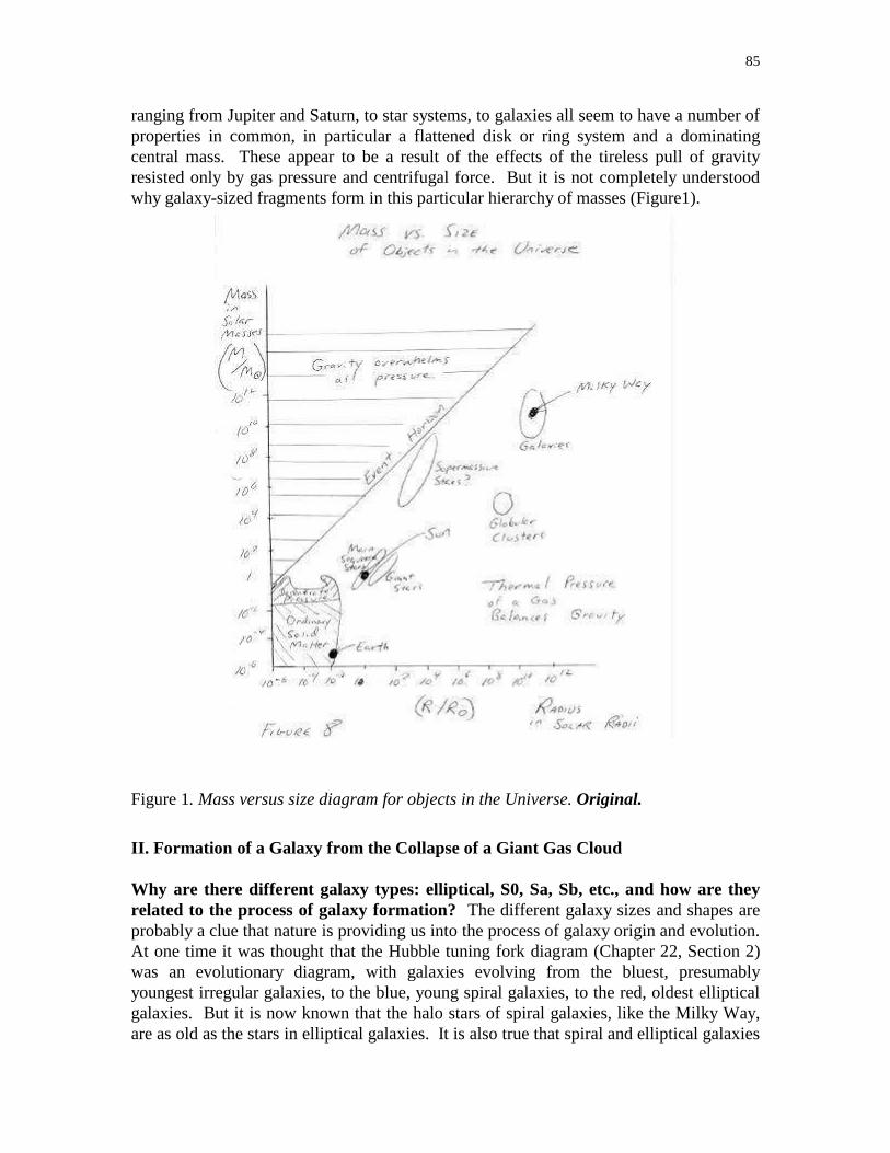
85

ranging from Jupiter and Saturn, to star systems, to galaxies all seem to have a number of

properties in common, in particular a flattened disk or ring system and a dominating

central mass. These appear to be a result of the effects of the tireless pull of gravity

resisted only by gas pressure and centrifugal force. But it is not completely understood

why galaxy-sized fragments form in this particular hierarchy of masses (Figure1).

Figure 1. Mass versus size diagram for objects in the Universe. Original.

II. Formation of a Galaxy from the Collapse of a Giant Gas Cloud

Why are there different galaxy types: elliptical, S0, Sa, Sb, etc., and how are they

related to the process of galaxy formation? The different galaxy sizes and shapes are

probably a clue that nature is providing us into the process of galaxy origin and evolution.

At one time it was thought that the Hubble tuning fork diagram (Chapter 22, Section 2)

was an evolutionary diagram, with galaxies evolving from the bluest, presumably

youngest irregular galaxies, to the blue, young spiral galaxies, to the red, oldest elliptical

galaxies. But it is now known that the halo stars of spiral galaxies, like the Milky Way,

are as old as the stars in elliptical galaxies. It is also true that spiral and elliptical galaxies

86

have differing angular momenta, making it improbable that one could evolve into the

other (Figure 2).

Figure 2. Angular momentum of galaxies versus type. Pearson.

If galaxies all evolved from clouds of gas under the same rules of physics, it might be

supposed that somehow the initial conditions or properties a gas cloud would determine

the eventual galaxy classification some ten billion years or so later. So the relevant

question might be: “How are galaxy types connected to the initial conditions of the

protogalactic gas cloud?” In particular it might be supposed that the balance

between gravity and spin would dominate the formation of a galaxy from a

collapsing gas cloud. Some of the initial conditions that we should look at are gas cloud

mass, density, and rate of spin.

Consider that a spinning cloud of gas will eventually collapse into a spinning disk, on a

galactic scale as on the scale of a star system. One of the most important parameters

in galaxy formation is the time it takes for stars to form, the star formation rate, vs.

the time it takes for a galaxy to collapse to a disk. It is important to note that in a

collapsing cloud, once a star is formed from a cloud fragment having a certain velocity,

this velocity will be frozen into the resulting star. Stars formed with orbits in the outer

87

reaches of the collapsing cloud will maintain these orbits in spite of cloud’s gas

collapsing to the cloud core. In essence, the collapsing gas will leave a generation of stars

behind it. In the collapsing cloud, gravity is balanced by angular momentum, or spin, and

gas pressure. Because the cloud is supported by spin only in directions perpendicular to

the spin axis, it will tend to collapse to a disk. If star formation occurs quickly, before

disk collapse, the galaxy will retain a roughly spherical shape. If it occurs slowly,

stars will form in the gas after it has collapsed into a disk, resulting in a spiral

galaxy.

The rate at which stars form probably depends on the density of gas in the collapsing

cloud at the time when galaxy formation commences. If a protogalactic cloud is dense, it

probably forms stars early, before disk collapse, and an elliptical galaxy results. If a

protogalactic cloud is sparse, the gas probably collapses while spinning up as angular

momentum is conserved (see also Chapter?) and most stars are formed subsequent to disk

collapse. Galaxy type is probably related to the local environmental conditions at the

time the galaxy formed: the density of the gas, and the amount of turbulence which

controls the size of protogalaxy fragments, their spin rate, and their density. Regions in

the Universe where gas density was low, such as in our Local Group, would tend to form

spiral galaxies, places where gas density was high, such as in rich galaxy clusters, would

tend to form elliptical galaxies with greater frequency. Indeed this is what is generally

observed.

III. Galaxy Formation in Two Waves: Star Populations

From Chapter 21, Section ? we found that the Milky Way can be grouped into two stellar

populations, representing two waves or generations of star formation: Population I stars,

the more recently formed, higher mass, generally bluer population of stars in the galactic

disk and Population II stars, the older, lower mass, redder population found concentrated

in the galactic halo. The nucleus and nuclear bulge contains stars of intermediate age

(Figure 3).

88

Figure 3. Population I and Population II stars in the Milky Way. Population I stars orbit

the center of the Galaxy in near circular orbits. Population II stars maintain a swarm of

elliptical and randomly inclined orbits. Modify. Hartmann and Impey.

Open Star Clusters

Located in the spiral arms of a galaxy

Small, typically composed of 1,000 solar masses of stars

Overall color ranges from blue to red

Ages range from young to old (10 billion years old is considered old)

Associated with clouds of dust and gas

Globular Star Clusters

In the halo of the Milky Way and other galaxies

Contain a large number of stars, typically 100,000 solar masses

Always red

All old (roughly 10 billion years old)

Have insignificant amounts of dust and gas

Elliptical galaxies contain almost exclusively Population II stars while spiral galaxies,

such as the Milky Way, contain both Population I and Population II components. (Figure

4.)

IV. Evidence for the Gravitational Collapse of Galaxy-Forming Gas Clouds

There is no single universally accepted theory of galaxy formation. But the most

generally accepted framework of how galaxies were formed is summarized in the

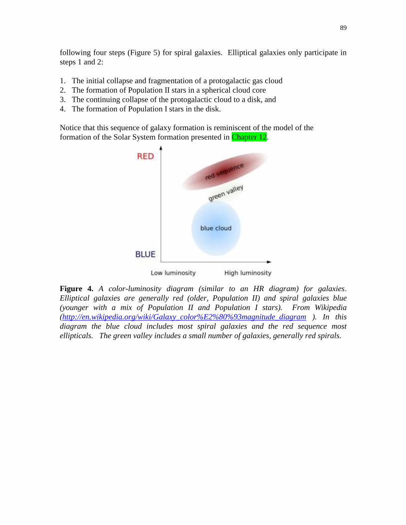
89

following four steps (Figure 5) for spiral galaxies. Elliptical galaxies only participate in

steps 1 and 2:

1. The initial collapse and fragmentation of a protogalactic gas cloud

2. The formation of Population II stars in a spherical cloud core

3. The continuing collapse of the protogalactic cloud to a disk, and

4. The formation of Population I stars in the disk.

Notice that this sequence of galaxy formation is reminiscent of the model of the

formation of the Solar System formation presented in Chapter 12.

Figure 4. A color-luminosity diagram (similar to an HR diagram) for galaxies.

Elliptical galaxies are generally red (older, Population II) and spiral galaxies blue

(younger with a mix of Population II and Population I stars). From Wikipedia

(http://en.wikipedia.org/wiki/Galaxy_color%E2%80%93magnitude_diagram ). In this

diagram the blue cloud includes most spiral galaxies and the red sequence most

ellipticals. The green valley includes a small number of galaxies, generally red spirals.

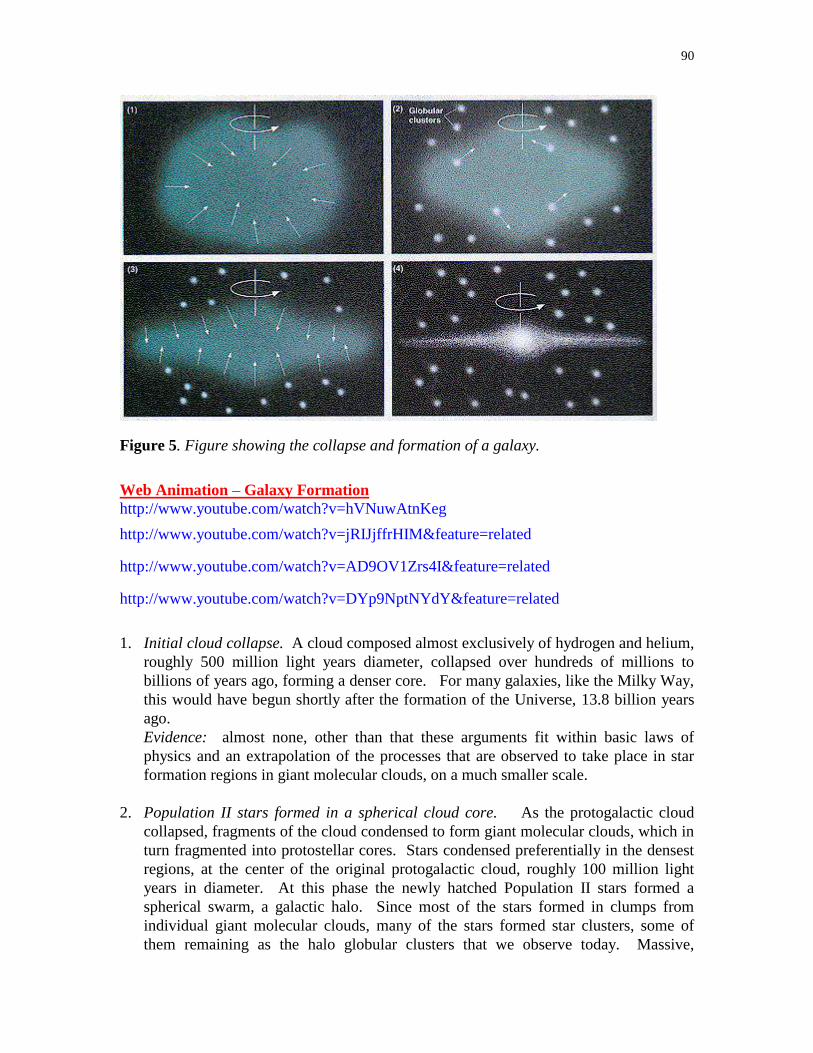
90

Figure 5. Figure showing the collapse and formation of a galaxy.

Web Animation – Galaxy Formation

http://www.youtube.com/watch?v=hVNuwAtnKeg

http://www.youtube.com/watch?v=jRIJjffrHIM&feature=related

http://www.youtube.com/watch?v=AD9OV1Zrs4I&feature=related

http://www.youtube.com/watch?v=DYp9NptNYdY&feature=related

1. Initial cloud collapse. A cloud composed almost exclusively of hydrogen and helium,

roughly 500 million light years diameter, collapsed over hundreds of millions to

billions of years ago, forming a denser core. For many galaxies, like the Milky Way,

this would have begun shortly after the formation of the Universe, 13.8 billion years

ago.

Evidence: almost none, other than that these arguments fit within basic laws of

physics and an extrapolation of the processes that are observed to take place in star

formation regions in giant molecular clouds, on a much smaller scale.

2. Population II stars formed in a spherical cloud core. As the protogalactic cloud

collapsed, fragments of the cloud condensed to form giant molecular clouds, which in

turn fragmented into protostellar cores. Stars condensed preferentially in the densest

regions, at the center of the original protogalactic cloud, roughly 100 million light

years in diameter. At this phase the newly hatched Population II stars formed a

spherical swarm, a galactic halo. Since most of the stars formed in clumps from

individual giant molecular clouds, many of the stars formed star clusters, some of

them remaining as the halo globular clusters that we observe today. Massive,

91

luminous stars aged quickly, over only millions of years, and evolved off the main

sequence. As these high mass stars exploded in supernovae they seeded the galaxy

with heavier elements and dust. As these massive blue stars died, the galaxy became

redder.

Evidence: this scenario is consistent with galaxy halo stars being red, heavy element

poor, and old. Halo stars are found above and below the disks of spiral galaxies.

Globular cluster H-R diagrams are consistent with computer models of stellar

evolution of an ancient generation of stars.

3. Disk collapse. Although the halo stars are orbiting the nucleus, the gas falls toward

the galaxy core inhibited only by gas pressure and angular momentum. As it falls, its

spin rate increases as it conserves angular momentum, as the ice skater pulling in his

or her arms increases their spin rate.

Evidence: little gas or dust is found in spiral galaxy halos or the nuclear bulge.

4. Gas and dust clouds are produced by self-gravitation. Population I stars formed

from the time of disk collapse until the present. Most recent star formation in spiral

galaxies has occurred along spiral arms. As the collapse of a spherical gas cloud

forms a spinning lens-shaped disk, the cloud becomes more enriched with metals

from dying Population II stars. Eventually the spin of the galaxy disk halts the

complete collapse of the cloud to the galaxy nucleus. Instead, gas, dust, and newly

forming stars are captured in a rotating disk. The newly-forming disk stars,

Population I stars, are enriched in heavy elements with gas recycled from the older

generation, Population II stars.

Evidence: this scenario is consistent with spiral galaxy disk stars being bluer, heavy

element enriched, and younger than the halo stars. The open clusters found in the

disks of galaxies have H-R diagrams that are consistent with computer models of

stellar evolution of stars formed after the halo stars formed. The most massive, blue

stars are found along spiral arms with the hydrogen clouds that these stars illuminate

and ionize.

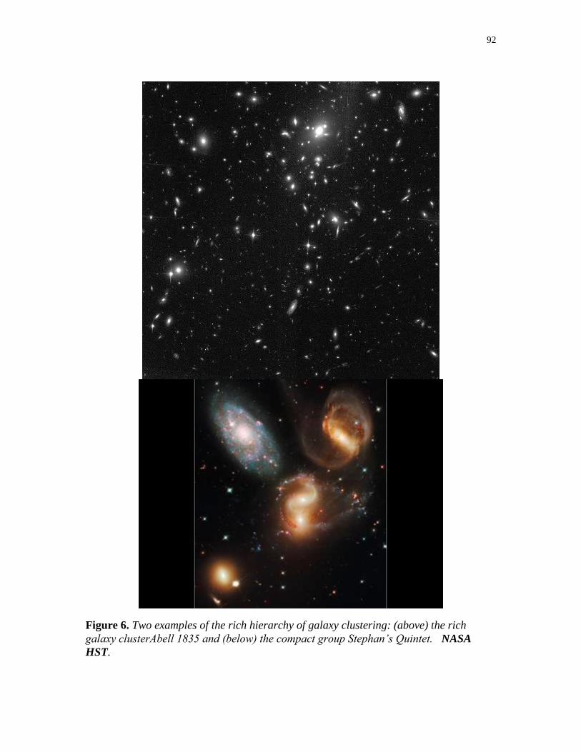
92

Figure 6. Two examples of the rich hierarchy of galaxy clustering: (above) the rich

galaxy clusterAbell 1835 and (below) the compact group Stephan’s Quintet. NASA

HST.

93

Other questions:

1) Why do objects have the mass hierarchy that they do? The British mathematician

and physicist James Jeans suggested a hierarchy of fragmentation, large objects

fragment into smaller ones that in turn fragment. The hierarchy spans galaxy

superclusters, clusters of galaxies, star clusters, and stars (Figure 6). More recently,

David Layzer of Harvard has supplemented this idea with the notion that as massive

clouds of gas collapse and fragment into smaller clouds, at each turn the forming

objects cluster. At one end, as stars form out of a giant molecular cloud they cluster

into one or more star clusters. One can visualize a similar clustering on the most

massive scales. As a proto-supercluster mass fragments and forms cluster clouds,

these clouds would eventually organize into one or more developing superclusters of

galaxies. We see the fragmentation and gravitational organization continue even

down to planets and planetary satellites.

2) Where did all the dust and gas go in elliptical galaxies? Elliptical galaxies are

devoid of gas and dust. One would not expect star formation to be perfectly efficient

at consuming all of the dust and gas in a galaxy over a period of 10 billion years.

Evolving stars should be continuously putting gas and dust back into the interstellar

medium via stellar winds and other mechanisms (Chapter 19, Section III). One can

infer that gas and dust are being continually removed from elliptical galaxies. If so,

what is the mechanism for this removal?

3) Why is the star-formation rate so high in the Milky Way and other spiral

galaxies? The Milky Way could not have sustained its current star formation rate

throughout its entire 10 billion-year life. Is the star-formation rate sporadic, or is gas

in the disk somehow being replenished?

These last two questions suggest that the unseen environment of a galaxy may place a

large role in its evolution. The collisions between galaxies are thought to be one strong

influence.

V. Galactic Cannibalism

The Milky Way and Andromeda are 100,000 light years in diameter and 20 times farther

apart, or 2 million light years. In rich galaxy clusters thousands of galaxies can be packed

much more tightly (Figure 7). Galaxies in the Local Group move with random velocities

of roughly 60 km/s with respect to one another. The Milky Way and Andromeda galaxies

are on a collision course and are expected to collide in about four billion years. Such

events may be crucial to our understanding of galaxy evolution. Dramatic as it may seem,

as galaxies containing tens of billions of stars collide, the vast separation between stars in

a galaxy would make the actual impact between two stars in such a collision rare. Other

effects are more important in galaxy collisions. Giant clouds of dust and gas in two

colliding galaxies would slam into each other at velocities of 100s of kilometers per

second, stopping them immediately in their tracks with their energy of motion heating the

two clouds and exciting or even ionizing the gas. A high-velocity collision can strip the

dust and gas right out of two colliding galaxies.

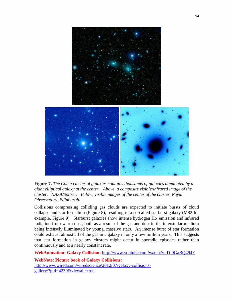
94

Figure 7. The Coma cluster of galaxies contains thousands of galaxies dominated by a

giant elliptical galaxy at the center. Above, a composite visible/infrared image of the

cluster. NASA/Spitzer. Below, visible images of the center of the cluster. Royal

Observatory, Edinburgh.

Collisions compressing colliding gas clouds are expected to initiate bursts of cloud

collapse and star formation (Figure 8), resulting in a so-called starburst galaxy (M82 for

example, Figure 9). Starburst galaxies show intense hydrogen H emission and infrared

radiation from warm dust, both as a result of the gas and dust in the interstellar medium

being intensely illuminated by young, massive stars. An intense burst of star formation

could exhaust almost all of the gas in a galaxy in only a few million years. This suggests

that star formation in galaxy clusters might occur in sporadic episodes rather than

continuously and at a nearly constant rate.

WebAnimation: Galaxy Collision: http://www.youtube.com/watch?v=D-0GaBQ494E

WebNote: Picture book of Galaxy Collisions:

http://www.wired.com/wiredscience/2012/07/galaxy-collisions-

gallery/?pid=4239&viewall=true

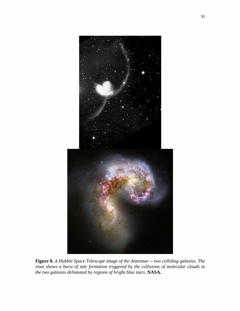
95

Figure 8. A Hubble Space Telescope image of the Antennae -- two colliding galaxies. The

inset shows a burst of star formation triggered by the collisions of molecular clouds in

the two galaxies delineated by regions of bright blue stars. NASA.

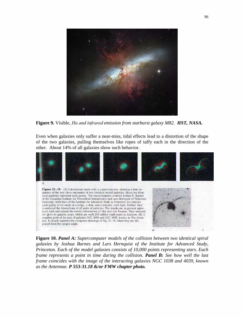
96

Figure 9. Visible, Hα and infrared emission from starburst galaxy M82. HST, NASA.

Even when galaxies only suffer a near-miss, tidal effects lead to a distortion of the shape

of the two galaxies, pulling themselves like ropes of taffy each in the direction of the

other. About 14% of all galaxies show such behavior.

Figure 10. Panel A: Supercomputer models of the collision between two identical spiral

galaxies by Joshua Barnes and Lars Hernquist of the Institute for Advanced Study,

Princeton. Each of the model galaxies consists of 10,000 points representing stars. Each

frame represents a point in time during the collision. Panel B: See how well the last

frame coincides with the image of the interacting galaxies NGC 1038 and 4039, known

as the Antennae. P 553-31.18 &/or FMW chapter photo.

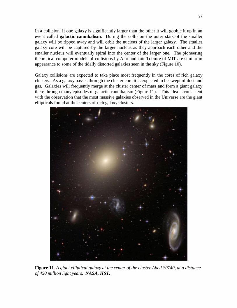
97

In a collision, if one galaxy is significantly larger than the other it will gobble it up in an

event called galactic cannibalism. During the collision the outer stars of the smaller

galaxy will be ripped away and will orbit the nucleus of the larger galaxy. The smaller

galaxy core will be captured by the larger nucleus as they approach each other and the

smaller nucleus will eventually spiral into the center of the larger one. The pioneering

theoretical computer models of collisions by Alar and Juir Toomre of MIT are similar in

appearance to some of the tidally distorted galaxies seen in the sky (Figure 10).

Galaxy collisions are expected to take place most frequently in the cores of rich galaxy

clusters. As a galaxy passes through the cluster core it is expected to be swept of dust and

gas. Galaxies will frequently merge at the cluster center of mass and form a giant galaxy

there through many episodes of galactic cannibalism (Figure 11). This idea is consistent

with the observation that the most massive galaxies observed in the Universe are the giant

ellipticals found at the centers of rich galaxy clusters.

Figure 11. A giant elliptical galaxy at the center of the cluster Abell S0740, at a distance

of 450 million light years. NASA, HST.

98

Summary

No one really knows how galaxies formed as they are with the masses and shapes that

they have. Astronomers generally believe that galaxies formed from the gravitational

collapse of giant clouds of gas, with masses of 100s of billions of suns, early in the

history of the Universe. Much of this model is based on theoretical results and the

observed fragmentation and collapse of much smaller clouds of gas and dust in the Milky

Way. One idea is that if star formation in a collapsing protogalaxy occurs quickly, before

disk collapse, the galaxy will retain a roughly spherical shape. If it occurs slowly, stars

will collapse into a disk, resulting in a spiral galaxy. A galaxy’s type is probably also

related to its environment, including its frequency of collisions with other galaxies.

We can divide galaxy formation into four phases: 1. the initial collapse and fragmentation

of a protogalactic cloud, 2. the formation of Population II stars in a spherical cloud core

3. the continuing collapse of the protogalactic cloud to a disk, and 4. the formation of

Population I stars in the disk.

Key Words & Phrases

1. galactic cannibalism – the collision of two galaxies where one galaxy gobbles up all

of the mass of the other

Review for Understanding

1.

Essay Questions

1. Why is it scientifically important for astronomers to be able to distinguish between

Population I and Population II stars?

Figure Captions

99

________________________________________________________________________

Chapter 26 – Observational Evidence for the Big Bang ________________________________________________________________________

Under heaven and Earth there is more than one can imagine.

--Shakespeare

What is inconceivable about the universe is that it is at all conceivable.

--Einstein

Chapter Preview

Some of the most interesting and fundamental questions in astronomy deal with the

Universe as a whole. How big is it? How old is it? How did it originate? How is it

evolving? It is mind-boggling that by measuring distances and properties of faraway

galaxies that we can use this information to build theories of the origin of our Universe,

the totality of all matter, radiation, and space that can be probed. What is even more

incredible is that these theories are testable. In this chapter we will examine the Big Bang

theory of the Universe, the theory that explains the observed velocity-distance

relationship for galaxies as the result of a Universe that formed some in a creation event.

An infinitesimally small and infinitely hot Universe expanded after this Big Bang. We

can still see the cosmic fireball radiation from this creation event 15 billion years ago.

100

Chapter Photo. An artist’s view of the formation of early universe with space populated

by protogalaxies and bubbles formed by the explosions of supernovae sending shock

waves out into the interstellar medium. Scaller, STSci.

Key Physical Concepts to Understand: General Relativity and cosmology, an

expanding Universe, determination of the age of the Universe, the steady state

cosmology, cosmic background radiation

I. Introduction

Never has so much been made from so little. From Slipher’s red shift measurements of

forty galaxies came the Hubble law describing the relationship between galaxy distance

and velocity measurements. From this small amount of data it was inferred that the

Universe has expanded and continues to expand from the creation event. A model of this

Big Bang has led for the first time to answers to some of the philosophical and previously

unanswerable fundamental questions of the origin and evolution of the Universe: What is

the global structure of the Universe? Is it evolving? Is it finite or infinite?

Newton believed the Universe to be infinite. He understandably looked at the Universe

through the perspective a scientist primarily concerned with gravity. If the Universe were

finite, why wouldn’t gravity cause it to collapse? He inferred that the matter in the

101

Universe must be distributed in infinite extent, so that the gravitational pull on any one

point would be zero, or equal in all directions. Gravity does indeed dominate the

structure of the Universe, and his concern with the collapse of the Universe was

prophetic.

One of the oldest and simplest cosmological tests is Olbers’ paradox. Olbers’ paradox

is misnamed, for it began as a question first posed by Edmund Halley in 1720, although it

is generally attributed to the German astronomer Wilhelm Olbers who lived a century

later. Olbers’ Paradox: In an infinite universe filled with stars, every line of sight

will eventually intercept the photosphere of a star. The result is that the entire sky

should be bright with the surface brightness of the average star. Why then is the

sky dark at night?

WebAnimation: Olber’s Paradox

http://upload.wikimedia.org/wikipedia/commons/d/d2/Olber%27s_Paradox_-

_All_Points.gif

Several solutions have been proposed to Olbers’ paradox over the years. One is that

interstellar dust serves to obscure distant stars, so that only stars that are relatively nearby

can be seen. The problem with this explanation is that any visible energy that is absorbed

by dust is eventually re-radiated in the infrared part of the spectrum. The sky is no more

intensely bright in the infrared than it is in the visible.

A more plausible explanation is that the Universe is not infinite but is only filled with

stars up to a finite distance. We know now that the Universe is not only finite in size, but

that the light from distant objects is red shifted. At great distances the light from galaxies

and the stars contained in them recede at velocities near the speed of light, reducing their

energy, as received by us, considerably.

II. General Relativity and Cosmology

Einstein’s theory of General Relativity (Chapter 20) was developed at a time when most

scientists considered the Universe to be static, or unchanging, at least as a whole. In 1917

Einstein applied his General Theory of Relativity to the Universe as a whole, and found

that to maintain a static Universe he needed to add a “cosmological constant”, or fudge

factor, to his equations, depending on one’s point of view.

102

Figure 1. The evolution of the size of the Universe for closed, open, and boundary Big

Bang Universes. If the Universe is open, it will increase in size forever. If it is closed its

expansion velocity is decelerating causing it to eventually reverse its expansion,

becoming smaller. An oscillating Universe is a special type of closed Universe that

repeats this cycle of expansion and contraction. In the case of a boundary Universe the

expansion continues forever but at an ever-decreasing rate. P 632-33.3.

In, 1919 the Dutch physicist W. de Sitter obtained a solution to Einstein’s cosmological

equations, without a cosmological constant, for the extreme case of a Universe with no

matter. In this solution, any particles introduced into this Universe would move apart

with velocities that would increase with time. In 1922 the Russian mathematician A.

Friedmann obtained the solutions to Einstein’s equations for matter-filled Universes, also

without a cosmological constant. The results were three classes of solutions: open, flat,

and closed Universes. We will assume that in each case the Universe begins as an

expansion from a singularity, which you can think of as a point. The open Universe is

characterized by an unbounded expansion from a point that continues forever (Figures 1

& 2). A closed Universe expands from a singularity, reaches a maximum size, and then

collapses into a singularity again. The flat Universe is the boundary between an open

Universe and a closed one. In a flat Universe, expansion proceeds from a singularity with

the expansion rate slowly at a decreasing rate, as the Universe forever approaches a fixed

size.

103

Figure 3. Snapshots of the Universe taken at several epochs after the Big Bang show the

formation of galaxies and the expansion of space.

Web Animation: Birth of the Universe

http://www.youtube.com/watch?v=NEZWtrvxyow&feature=related

http://www.youtube.com/watch?v=7WiBET8H3x0&feature=related

http://www.youtube.com/watch?v=uD8uFCQkpDE&feature=related

http://www.youtube.com/watch?v=gr8zLAxPs-A&feature=related

http://www.youtube.com/watch?v=_l0yxRRCrfk&feature=related

III. Galaxy Red Shifts and the Expansion of the Universe

The discovery by Hubble in 1929 that galaxies are moving away from each other with a

velocity in proportion to their distance (according to the Hubble law, velocity = H

distance, where H is the Hubble constant) was one of the major scientific discoveries of

the 20th

century. The Hubble law provided hard experimental verification to the Einstein

model of the Universe, without the cosmological constant. Einstein later confessed that

the addition of a cosmological constant to his equations was the biggest mistake of his

career. The distance red shift relationship also confirmed the Friedmann models of the

Universe.

Subsequent measurements have shown that all distant galaxies are moving away

from us and that the Hubble law is the same in all directions. Does this mean that

104

all galaxies in the Universe are expanding with the Milky Way at the center? There

has been a constant historical tendency for humans to regard the Earth as the center of the

Universe, or the Sun as the center of the Milky Way, or now, the Milky Way as the center

of the Universe. This assumption was found to be in error in the first two cases, and we

will soon see it is not true in the third case either.

A. Raisin Bread Model of the Universe - an Ant’s Perspective

Figure 4. Panel A: A raisin bread model of the Universe. In a loaf of rising raisin bread

as in a Big Bang Universe, an ant standing on any raisin would see all the other raisins

moving away such that the farther the distant raisin, the faster the ant sees it move. FMW

515-25.18 Modified. Panel B: Hubble law for raisins. Original.

To see how an expanding Universe would look from anywhere in the Universe, we’ll

model it in more familiar terms. Imagine the Universe as a loaf of rising raisin bread with

raisins dotting the interior of the bread with a uniform spacing (Figure 4). We’ll consider

raisins to be galaxy analogs. But wait! On one raisin is attached an unsuspecting ant,

munching away with little concern. We are that ant. We will assume that the bread is

expanding at a uniform rate. Initially the raisins are spaced 1 centimeter apart. As the

bread rises the spacing changes, to 2 cm in 15 minutes, 3 cm in 30 minutes and so on. If

we look at the raisins along one line of sight we can measure their distance and the rate at

which they recede (Table 26.1). Using the data in Table 26.1 we can plot the velocity vs.

distance for raisins along this same line of sight. The result is a Hubble law for raisin

bread (with apologies to Edwin Hubble). Notice that we have assumed nothing about the

position of our raisin in the bread or the direction of the line of sight. The Hubble law is

valid for any direction in the raisin bread and from the viewpoint of any raisin. It is not

correct to infer from the observations that one is sitting on some central or preferred raisin

in the bread. Our raisin has no philosophical significance.

WebAnimation: Expanding Raisin Bread

http://en.wikipedia.org/wiki/File:Raisinbread.gif

105

Table 26.1: The Raisin Bread Recipe for an Expanding Universe

Raisin Time = 0 1 hour 2 hours 3 hours 4 hour

#1 position 1 cm 2 cm 3 cm 4 cm 5 cm

velocity 1 cm/hr

#2 position 2 cm 4 cm 6 cm 8 cm 10 cm

velocity 2 cm/hr

#3 position 3 cm 6 cm 9 cm 12 cm 15 cm

velocity 3 cm/hr

B. The Improved Balloon Model of the Universe – a Finite but Unbounded Universe

The curvature of space-time produces a finite but unbounded expanding Universe that

cannot be adequately illustrated with the raisin bread analogy. We will upgrade our

model to a more sophisticated balloon model of the Universe to take into account the

curvature of space.

As three-dimensional creatures there is no adequate way to visualize the curvature of a

three dimensional space. It can be conceptually illustrated by the consideration of the

curvature of a two dimensional space. Imagine that we live as paper-thin two

dimensional creatures that work and live in a two-dimensional surface, able to think in

terms of North and South but unable to conceive of up or down. On a local scale our

Universe seems flat and extends without limit in all directions. On a universal scale the

Universe is spherical and can be modeled as the surface of a balloon. Our Universe is

also an expanding one, the sphere, or balloon surface, growing in diameter at a constant

rate as it is being blown up (Figure 5).

To us the inside and outside of our spherical surface have no significance. As we begin

to explore our Universe we can leave our residences and walk in a straight line,

eventually to return to the exact spot from which we started. This occurs because we live

in a curved space, unbounded but of finite extent.

As the balloon expands we can measure the distances and velocities between points on

the surface of a balloon as we could in the rising raisin bread. The velocities correspond

to the cosmological red shifts that we see in our own Universe. The results are the same

as those in Table 26.1 and result in a Hubble law for an expanding two-dimensional space

(Figure 5).

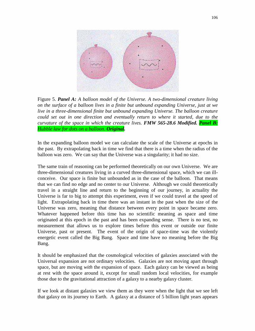
106

Figure 5. Panel A: A balloon model of the Universe. A two-dimensional creature living

on the surface of a balloon lives in a finite but unbound expanding Universe, just at we

live in a three-dimensional finite but unbound expanding Universe. The balloon creature

could set out in one direction and eventually return to where it started, due to the

curvature of the space in which the creature lives. FMW 565-28.6 Modified. Panel B:

Hubble law for dots on a balloon. Original.

In the expanding balloon model we can calculate the scale of the Universe at epochs in

the past. By extrapolating back in time we find that there is a time when the radius of the

balloon was zero. We can say that the Universe was a singularity; it had no size.

The same train of reasoning can be performed theoretically on our own Universe. We are

three-dimensional creatures living in a curved three-dimensional space, which we can ill-

conceive. Our space is finite but unbounded as in the case of the balloon. That means

that we can find no edge and no center to our Universe. Although we could theoretically

travel in a straight line and return to the beginning of our journey, in actuality the

Universe is far to big to attempt this experiment, even if we could travel at the speed of

light. Extrapolating back in time there was an instant in the past when the size of the

Universe was zero, meaning that distance between every point in space became zero.

Whatever happened before this time has no scientific meaning as space and time

originated at this epoch in the past and has been expanding sense. There is no test, no

measurement that allows us to explore times before this event or outside our finite

Universe, past or present. The event of the origin of space-time was the violently

energetic event called the Big Bang. Space and time have no meaning before the Big

Bang.

It should be emphasized that the cosmological velocities of galaxies associated with the

Universal expansion are not ordinary velocities. Galaxies are not moving apart through

space, but are moving with the expansion of space. Each galaxy can be viewed as being

at rest with the space around it, except for small random local velocities, for example

those due to the gravitational attraction of a galaxy to a nearby galaxy cluster.

If we look at distant galaxies we view them as they were when the light that we see left

that galaxy on its journey to Earth. A galaxy at a distance of 5 billion light years appears

107

as it did 5 billion years ago. Nonetheless, observers on all galaxies in the Universe could

agree on a universal time scale, say number of years after the Big Bang. Each observer in

the Universe would see a similar local Universe at any given epoch of cosmic universal

time, but would view earlier epochs when looking out at distant galaxies, as a result of the

finite velocity of light. Aliens on other galaxies might now being viewing the Milky Way

as a quasar because they are viewing the Milky Way as it looked billions of years ago.

The fact that we can only see distant stars and galaxies as far as the look-back time

corresponding to the age of the Universe is the resolution to Olbers’ paradox; the

Universe is not infinite.

IV. Age of the Universe

In the 1940s, American Physicist George Gamow proposed that the Universe began in an

explosion, which we now call the Big Bang. When did the Big Bang occur? A simple

calculation gives us an estimate of the length of time that has passed since the Big Bang.

If we reverse the cosmological expansion by going back in time, the galaxies were closer

together in the past; at times near the time of the Big Bang all matter, all points in space,

were in the same neighborhood. At the time of the Big Bang, there was zero distance

between any two points. The age of the Universe can be calculated by assuming that the

distance between any two points in the expanding Universe is equal to the age of the

expansion times the relative expansion velocity between the two points. We can use the

distance between a distant galaxy and the Milky Way and the velocity that the distant

galaxy has been receding to calculate the age of the Universe:

Equation 26.1: Age of the Universe = galaxy distance/galaxy velocity.

But rearranging the Hubble law gives us, H = galaxy velocity/galaxy distance.

Combining Equation 26.1 with the Hubble law produces the following:

Equation 26.2: Age of the Universe = 1/H.

With the currently accepted Hubble constant of 75 km/s/megaparsec we compute an age

of 13 billion years. It is comforting that this age is longer than the age of the Solar

System and the modeled ages of the oldest stars in the Milky Way. If it were otherwise

there would be a contradiction.

Math box: Let’s estimate the age of the Universe from H.

If the age of the Universe is 1/H and H = 75 km/s/megaparsec, then we can determine the

age by the following:

1 megaparsec = 3 1019

km, so

age of the Universe = 1/H = 1 / 75 km/s/ 3 1019

km = 4 1017

seconds

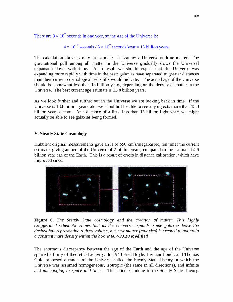
108

There are 3 107 seconds in one year, so the age of the Universe is:

4 1017

seconds / 3 107 seconds/year = 13 billion years.

The calculation above is only an estimate. It assumes a Universe with no matter. The

gravitational pull among all matter in the Universe gradually slows the Universal

expansion down with time. As a result we should expect that the Universe was

expanding more rapidly with time in the past; galaxies have separated to greater distances

than their current cosmological red shifts would indicate. The actual age of the Universe

should be somewhat less than 13 billion years, depending on the density of matter in the

Universe. The best current age estimate is 13.8 billion years.

As we look further and further out in the Universe we are looking back in time. If the

Universe is 13.8 billion years old, we shouldn’t be able to see any objects more than 13.8

billion years distant. At a distance of a little less than 15 billion light years we might

actually be able to see galaxies being formed.

V. Steady State Cosmology

Hubble’s original measurements gave an H of 550 km/s/megaparsec, ten times the current

estimate, giving an age of the Universe of 2 billion years, compared to the estimated 4.6

billion year age of the Earth. This is a result of errors in distance calibration, which have

improved since.

Figure 6. The Steady State cosmology and the creation of matter. This highly

exaggerated schematic shows that as the Universe expands, some galaxies leave the

dashed box representing a fixed volume, but new matter (galaxies) is created to maintain

a constant mass density within the box. P 607-33.10 Modified.

The enormous discrepancy between the age of the Earth and the age of the Universe

spurred a flurry of theoretical activity. In 1948 Fred Hoyle, Herman Bondi, and Thomas

Gold proposed a model of the Universe called the Steady State Theory in which the

Universe was assumed homogeneous, isotropic (the same in all directions), and infinite

and unchanging in space and time. The latter is unique to the Steady State Theory.

109

Galaxies would recede from each other with apparent velocities in proportion to their

distance, obeying Hubble’s law. Essentially, the Steady State Universe is an infinite

Universe that expands. Ordinarily this expansion would cause a decreasing density of

matter in the Universe. In order to maintain an unchanging Universe, the density of

matter should be constant. It was proposed by Hoyle, Bondi, and Gold that matter would

need to be created continuously throughout the Universe to maintain a constant density

(Figure 6). Although this theory seems unsettling, it can be argued that it is no more

settling than the sudden creation of the Universe in the Big Bang. The direct creation of

matter in the Steady State Theory only amounted to about 1 atom per cubic meter every

billion years or so, so that it would be undetectable. The debate between the Big Bang

and Steady State theories lasted until 1964.

VI. Cosmic Background Radiation

After World War II American physicist Ralph Alpher and Russian-American physicist

George Gamow proposed that the Universe immediately after the Big Bang was

incredibly hot, filled with high intensity high energy photons called the cosmic

background radiation. As the universe expanded the cosmic background radiation cooled

as the radiation was red shifted (Figure 7).

Figure 7. Figure showing blackbodies at various red shifts corresponding to cosmic

background radiation. Original.

In 1964 Arno Penzias and Robert Wilson, Bell Telephone Laboratory physicists, built a

microwave antenna to relay phone calls from Earth-orbiting satellites. They detected a

signal emanating from the sky in all directions. They initially discounted this to noise.

After laboriously trying to eliminate this noise from their antenna, a colleague informed

them of the previous predictions of the cosmic background radiation by Alpher and

Gamow. Penzias and Wilson are credited with the first detection of the cosmic

background radiation. This detection of cosmic fireball radiation was the first

experimental verification of the Big Bang independent of the velocity red shift

relation.

110

More recent and precise measurements of the cosmic background show that it has a

blackbody spectrum with a temperature of 2.73 degrees. It is commonly referred to as the

3-degree background radiation.

After the Big Bang, the matter and radiation in the Universe cooled as the Universe

expanded. In the Alpher and Gamow theory, about 700,000 years after the Big Bang the

Universe would cool to about 4,000 K, cool enough for electrons to combine with

individual protons forming hydrogen atoms. Individual charged electrons and protons are

relatively opaque to electromagnetic radiation. When electrons and protons combine to

form uncharged hydrogen atoms they become quite transparent to most electromagnetic

radiation. When the Universe was opaque, in the first 700,000 years after the Big Bang,

frequent interactions between light and matter, in which photons scattered off of electrons

and protons, forced matter and radiation to be confined to the same volumes of space. As

matter cooled and formed uncharged hydrogen atoms, light and matter were free to go

their own ways, and matter, no longer pushed around by light as in some cosmic blender,

was free to collapse into condensations. When light and matter uncoupled, theory

predicts that radiation would have had a blackbody spectrum of 3,000 – 4,000 K.

Figure 8. Panel A: A COBE (Cosmic Background Explorer) cosmic background

spectrum compared to a 2.73 K blackbody. FMW 575-28.15 or P 612-33.16. Panel B:

The COBE satellite. P 612-33.15.

The cosmic background radiation filled all of space. When we observe the cosmic

background radiation today we are looking a radiation coming from a distance

corresponding to the look-back time of the age of the Universe minus 700,000 years, just

as when we look at a galaxy at a distance of 5 billion light years we are looking back 5

billion years in time. The only difference is that a galaxy is seen only in one direction in

space, the cosmic background radiation comes from all directions because it fills space.

The 4,000 K background radiation should experience the same kind of cosmological red

shift that galaxies do. The radiation we observe 700,000 years after Big Bang would be

red shifted by 1,000, from the visible to a wavelength of about a millimeter, from 4,000 K

111

to nearly 3 K. It was this millimeter wavelength radiation that was detected by Penzias

and Wilson, and for which they won the 1978 Nobel Prize in physics.

Figure 9. A COBE map of the Universe showing the anisotropy of the cosmic

background. FMW chapter cover or APOD, NASA.

The Cosmic Background Explorer satellite, COBE, was launched in 1989 to map the

cosmic background radiation (Figure 8). COBE has shown that the cosmic background is

isotropic with the exception of an additional red shift in one direction due to the velocity

of the Earth about the Sun, the Sun about the center of the Milky Way, and the Milky

Way through the Universe. The entire Milky Way appears to be moving 600 km/s

relative to the neighboring Universe as the Milky Way and Local Group appear to be

pulled towards four nearby clusters and a massive supercluster (Figure 9).

In the next chapter we will also see that the abundances of lithium and helium in stars

agree with the predictions of the Big Bang theory.

112

Summary

The Theory of General Relativity was developed by Einstein in 1917 and used by de

Sitter in 1919 and Friedmann in 1922 to show that the natural state of the Universe is one

of the expansion of space. This was confirmed by Hubble in 1929 who discovered that

galaxies are moving away from each other with a velocity in proportion to their distance.

The age of the Universe can be calculated by assuming that the distance between any two

points in the expanding Universe is equal to the age of the expansion times the relative

expansion velocity between the two points. The current estimated age of the Universe is

15 billion years.

In 1948 Hoyle, Bondi, and Gold proposed the Steady State Cosmology in which the

Universe was assumed to be infinite and expanding, obeying the Hubble law. To

maintain a constant density of the Universe this required the continuous creation of

matter.

Supporting proof of the Big Bang Cosmology came with the discovery of the cosmic

background radiation, a 2.73 K background radiation that fills all of space. This fossil

radiation from the Big Bang was predicted by the model of Alpher and Gamow, which

assumed an initial Universe that was infinitely hot and infinitesimally small at the

moment of creation.

Key Words & Phrases

1. cosmological constant – the constant added to Einstein’s General Theory of

Relativity to keep the Universe from expanding

2. Olbers’ paradox – The paradox which says that in an infinite, unchanging Universe

filled with stars, the sky should appear bright at night

3. Singularity

4. 3-degree background radiation – cosmic fireball radiation from the Big Bang that

has been red shifted so that it has an intensity distribution with wavelength like a

2.73-degree blackbody

Review for Understanding

1. What is the difference between 1/H and the actual age of the Universe (for the

moment of the Big Bang)? Which is greater?

2. List observational evidence in favor of and against each of the following: (a) the Big

Bang Theory, and (b) the Steady State Theory.

3. What is Olbers’ paradox? What does it tell us?

113

4. What is the Steady State Cosmology? How do we know it is incorrect?

Essay Questions

1. If you were located in a galaxy near the boundary of our observable Universe, would

the galaxies in the direction of the Milky Way appear to be approaching or receding

from you? Explain.

Figure Captions

Figure 6. Drawing of look-back time and galaxy evolution. Original.

114

________________________________________________________________________

Chapter 27 – Origin and Evolution of the Universe ________________________________________________________________________

Nature is an infinite sphere, whose center is everywhere and whose circumference is

nowhere.

--Pascal (1670)

God writes straight with curves.

--Freemason philosopher (1782)

Truth in science can be defined as the working hypothesis best suited to open the way to

the next better one.

--Konrad Lorenz

Chapter Preview

In this chapter we will look in more detail at the early stages after the Big Bang, including

the creation of matter and of four separate forces in nature: gravity, the electrical force,

the strong force, and the weak force. The Big Bang theory predicts that the creation of

the light elements, hydrogen, helium, and lithium, occurred during the first three or four

minutes after the birth of our Universe. These elements were essentially produced by the

transformation of light into matter. The character of our Universe was formed during the

initial few seconds of its life. The study of this period weds cosmology, the study of the

Universe as a whole, with high-energy nuclear physics, the study of the most elementary

building blocks of matter.

Key Physical Concepts to Understand: creation of matter, decoupling of matter and

radiation, Grand Unified Theory of forces, pair production, inflation, critical density,

dark matter, determination of the deceleration of the Universe

I. Introduction

In the previous chapter the Big Bang theory of the Universe was introduced. The Big

Bang theory originated with the discovery by Hubble of the expansion of the Universe

and the theoretical models by Einstein, de Sitter, and Friedmann of an expanding

Universe. This work spurred the work of Alpher and Gamow, the theory that predicted

the formation of matter in a cooling Universe, later verified by the discovery of the

microwave background by Penzias and Wilson. Additional verification of Alpher and

Gamow’s theory is the measured composition of the oldest stellar populations in galaxies,

75% hydrogen and 25% helium. In this chapter we will examine in more detail the theory

of the origin and evolution of matter and radiation as well as forces in the current, more

refined models of modern cosmology (Figure 1).

115

Figure 1. A detailed timeline of the history of the Universe. FMW 626-34.13.

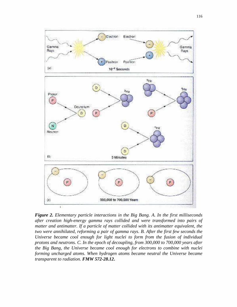
116

Figure 2. Elementary particle interactions in the Big Bang. A. In the first milliseconds

after creation high-energy gamma rays collided and were transformed into pairs of

matter and antimatter. If a particle of matter collided with its antimatter equivalent, the

two were annihilated, reforming a pair of gamma rays. B. After the first few seconds the

Universe became cool enough for light nuclei to form from the fusion of individual

protons and neutrons. C. In the epoch of decoupling, from 300,000 to 700,000 years after

the Big Bang, the Universe became cool enough for electrons to combine with nuclei

forming uncharged atoms. When hydrogen atoms became neutral the Universe became

transparent to radiation. FMW 572-28.12.

117

II. Thermonuclear Detonation first 3 minutes

Web Animation: The First Three Minutes

The First Few Seconds. The currently accepted scenario for the Big Bang Universe is

that the Universe was created in a singular event approximately 13 billion years ago. The

Universe was created as an infinitesimal but expanding space filled with energy. During

the first few seconds in the life of our Universe the temperature of matter and photons

was billions of Kelvins, so hot that neutrons and protons could not be bound together for

more than a moment before they would be smashed apart by colliding particles or blown

apart by super-energetic gamma rays (Figure 2). The Universe during the first seconds

was an ocean of gamma ray photons, electrons, protons, neutrinos and other elementary

particles. Photons were more common than particles by a billion to one, resulting in what

physicists call a radiation-dominated Universe. The state of matter was controlled by the

existence of high-energy photons. At this point the entire Universe was no larger than the

Sun.

The First Few Minutes. After a minute the temperature of the Universe was roughly 1

billion K, cool enough for the strong force to hold particles together against the

absorption of radiation and high-velocity collisions with other particles. Neutrons and

protons combined to form a single nucleus, deuterium (heavy hydrogen, with a nucleus

of one proton and one neutron). Deuterium nuclei were able to capture additional

particles, forming tritium (another hydrogen isotope with a nucleus of one proton and

two neutrons), helium-3 (two protons and 1 neutron), and helium-4 (ordinary helium with

two protons and two neutrons). Nearly all of the nucleus-building that would occur in the

early Universe happened during the first four minutes or so. The gross composition of

early Universe was frozen at 75% helium and 25% hydrogen, by mass. In the next 30

minutes, trace amounts of lithium-7 (3 protons, 4 neutrons) and beryllium-7 (4 protons, 3

neutrons) formed+, then nuclear reactions halted, as the Universe was too cool and thin to

support the high-velocity collisions that are required to fuse nuclei from constituent

particles. All of the heavier elements, such as carbon and oxygen, were produced later in

the interiors of stars.

Is this theory matched by observations? Although helium is produced from the fusion

of hydrogen in main sequence stars, spectroscopy of the oldest stars in our galaxy and in

the oldest and most unevolved nearby galaxies show a helium abundance of 25% by mass

with little variation. The Big Bang theory predicts that helium is 100 million times more

common than lithium. This is also supported by observations.

Deuterium production is sensitive to the density of the Universe at the time that it formed,

since it is easily created and destroyed by collisions with other particles. A predicted

deuterium abundance of one in 50,000 atoms is hard to detect. Deuterium is also easily

destroyed in stellar interiors. The result is that it is difficult to use deuterium to confirm

or deny the Big Bang theory.

118

III. The Radiation Era – the First 300,000 Years

Radiation dominated the expanding Universe for thousands of years with little qualitative

change. The sea of electrons and nuclei was far too hot for electrical attraction to bind

electrons to nuclei. As the Universe expanded, the radiation temperature dropped as the

wavelength of photons was stretched to longer and longer wavelengths. At an age of one

year, the temperature of the Universe was several million Kelvins and it was filled with

X-ray radiation. At an age of several thousand years the temperature cooled to 100,000 K

and contained primarily ultraviolet radiation.

IV. Decoupling of Matter and Radiation

300,000 years after the Big Bang, the temperature of the Universe had fallen to 3,000 to

4,000 K, with cosmic background photons red shifted into the visible part of the

electromagnetic spectrum. The universe was opaque prior to this time, with radiation

easily absorbed by unattached electrons and protons, charged particles acting as little

absorbing antennae. The temperature at earlier epochs was high enough to keep electrons

and protons from combining to form hydrogen atoms. As the Universe cooled and

electrons and protons combined to form uncharged atoms, the Universe suddenly became

transparent to light. Electrically neutral hydrogen atoms are transparent to light except at

those few discrete wavelengths where absorption lines exist.

What do we see when we look as far out into space as we can, with large telescopes?

As we look out in distance we look back in time. What is the earliest epoch that can be

detected? We can see the cosmic fireball radiation as it was at the time 300,000 years

after the Big Bang when the Universe became transparent. At this time radiation

separated from matter and was free to travel in one direction at the speed of light. Prior to

this time the Universe was an expanding opaque fog of absorbing particles that hid itself

from view. When looking back in time we can only “see” the radiation leaving this fog

behind, the rest is forever hidden from view.

Since the time when hydrogen atoms formed and matter and radiation decoupled, the

Universe has grown a thousand times bigger and the cosmic background radiation has

cooled by a factor of 1,000 (or alternatively, the cosmic background has been red shifted

by a factor of 1,000). Photons from the cosmic fireball have red shifted to the microwave

portion of the electromagnetic spectrum as its blackbody temperature has cooled from

3000 K to 3 K. The Universe has become matter dominated, although number of cosmic

background photons remains the same. The total energy wrapped up in these photons has

appeared to steadily decrease as they have become more and more red shifted.

V. The Formation of Matter and GUT

119

In the contemporary Universe there are four known forces: gravity, electrical force, and

the strong and weak nuclear forces. Gravity holds the Universe together on a large scale,

decelerating the expansion of the Universe as a whole and collecting matter into galaxy

clusters, galaxies, stars, and planets. The electrical force attracts particles of opposite

charge, binding atoms together as a family of protons and their orbiting electrons. Over

large distances electrical forces are usually insignificant as equal numbers of protons and

electrons in a given region will cancel each other’s charge, producing the same

cumulative effect as no charge. This doesn’t happen for gravity, which does not come in

two flavors, so it’s effects simply accumulate and are seen on the largest scales. The

strong force operates only in the close confines of the atomic nucleus, binding neutrons

and protons into separate and distinct elements. The effects of the weak nuclear force are

only evident in some kinds of reactions where an unstable nucleus decays. Both the weak

and strong forces are only effective over distances of 10-15

m or less.

Figure 3. Quarks make up protons and neutrons. A schematic. P 623-34.7.

Protons and neutrons are themselves composed of more elementary building blocks, or

sub-particles, called quarks (Figure 3). The proton, for example, is composed of three

quarks, two up quarks and one down quark (the up and down have no real significance,

they are simply a whimsical naming convention). The neutron is composed of two down

quarks and one up quark. The weak forces act whenever one quark changes such as when

a neutron forms a proton.

Experimental examination of the reactions that occurred in the Universe within the first

second of its birth requires the largest nuclear accelerators, which can collide particles at

velocities near the speed of light. At these velocities it is seen that the four known forces

begin to act in the same way. For example, a series of experiments at the European

CERN accelerator in the 1980s showed that at the highest particle energies the weak and

nuclear forces had the same strength. It has been proposed in theory, generally referred to

as the Grand Unified Theory, or simply GUT, that all four forces would have the same

strength at the ultra-high particle energies in the early Big Bang, which cannot be

replicated on Earth (Figure 4).

120

Figure 4. A timeline of the evolution of four forces in the period immediately after the

creatio4 of the Universe. At the high energies corresponding to times immediately after

the Big Bang the four known forces were indistinguishable. As the Universe cooled four

forces with separate and distinguishable characteristics evolved. From

http://hyperphysics.phy-astr.gsu.edu.

At times ranging from t = 0 to10-43

seconds after the Big Bang, the so-called Planck

time, named after the father of quantum theory, Max Planck, it is theorized that there was

only one unified force. At t = 10-32

s and a Universe temperature of 1032

K, gravity

separated into a force distinct from the other three: a combined electrical-strong-weak

force. At 10-35

s and a temperature of 1027

K the strong nuclear force separated from the

electro-weak force and appeared as separate and distinct. At t=10-35

to 10-24

s an abrupt

expansion of the Universe, called inflation, occurred, and the size of the Universe

expanded by 1050

in size. We will study inflation in more detail in the next section. At

t=10-12

s and 1015

K the electromagnetic force and weak force separated; the Universe had

four independent forces for the first time. Prior to t=10-6

s and 1013

K the Universe was

too hot for protons and neutrons to exist; matter existed only as individual quarks. After

this epoch the Universe was cool enough for quarks to stick together in individual protons

and neutrons.

During the 1st second both matter and antimatter could be created. What is antimatter?

For each elementary particle there is an equivalent anti-particle. For the proton there is a

corresponding anti-proton, a particle with the same mass as the proton but negative

charge. Corresponding to the electron, is the positron, an oppositely charged, same mass

antimatter equivalent. For the neutron there is the anti-neutron; neither has charge.

121

Antimatter is seen in the laboratory in experiments that produce high-energy gamma rays.

As two gamma rays of the right energy collide they produce a particle and its anti-

particle, transforming energy, in the form of two gamma-ray photons, into matter, a pair

of elementary particles, electron-positron, proton-antiproton, etc. This process is called

pair production (Figure 2). If a particle and its antiparticle collide, the two will

annihilate each other, forming high-energy photons; the result is the conversion of matter

back into energy.

At times earlier than 1 second, pair production occurred frequently producing matter and

anti-matter in nearly equal amounts. After t=1 s, pair production ceased as the Universe

cooled to a temperature where their was little if no production of gamma-rays of high

enough energy to support the process. If both matter and antimatter were produced in

equal numbers in the early Universe, why aren’t they found in equal numbers now?

Why does the Universe appear to be exclusively matter? There is no evidence of

patches of antimatter bordering on regions of ordinary matter with a boundary layer

separating the two where annihilation is producing large numbers of gamma ray photons.

Physicists expect that in pair production the number or particles formed was slightly

larger than the number of anti-particles, by, say, one part in a billion. After pair

production and matter/anti-matter annihilation ceased, the Universe then contained

exclusively the extra matter leftover from the annihilation process.

After the first second, protons, neutrons, and electrons collided and fused forming nuclei.

During the first three minutes they were broken apart by high-energy collisions and

absorption of gamma rays. After the first three minutes the abundances were frozen in

and no further fusion occurred. The Universe was too cool for collisions or radiation to

break the bonds formed by the strong force.

For the first 300,000 years relatively high-energy photons kept neutral atoms from

forming. After the radiation-dominated era, the Mixmaster of the Universe, photons,

which had previously pushed matter around and kept the Universe somewhat

homogenous, found matter to be transparent. The matter in the Universe was no longer

continuously mixed and gravity took over, causing the clumping of matter into

superclusters, clusters, galaxies, star clusters, stars, and planets. Clumps of matter formed

from rapidly cooling and thinning matter.

V. Inflation

The near-isotropy of the cosmic fireball radiation creates a problem for the Big Bang

theory. With a current diameter of 30 billion light years, why do opposite sides of

the Universe have almost exactly the same temperature? Since the Big Bang they

have evolved independently and in isolation to each other. Scientists expected

temperature differences on the sky as to vary from place to place as they evolved along

slightly different paths.

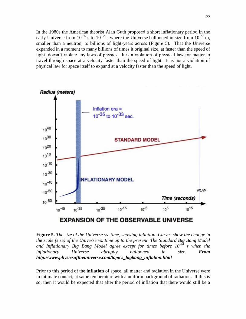
122

In the 1980s the American theorist Alan Guth proposed a short inflationary period in the

early Universe from 10-35

s to 10-33

s where the Universe ballooned in size from 10-27

m,

smaller than a neutron, to billions of light-years across (Figure 5). That the Universe

expanded in a moment to many billions of times it original size, at faster than the speed of

light, doesn’t violate any laws of physics. It is a violation of physical law for matter to

travel through space at a velocity faster than the speed of light. It is not a violation of

physical law for space itself to expand at a velocity faster than the speed of light.

Figure 5. The size of the Universe vs. time, showing inflation. Curves show the change in

the scale (size) of the Universe vs. time up to the present. The Standard Big Bang Model

and Inflationary Big Bang Model agree except for times before 10-30

s when the

inflationary Universe abruptly ballooned in size. From

http://www.physicsoftheuniverse.com/topics_bigbang_inflation.html

Prior to this period of the inflation of space, all matter and radiation in the Universe were

in intimate contact, at same temperature with a uniform background of radiation. If this is

so, then it would be expected that after the period of inflation that there would still be a

123

uniform background of radiation characterized by a single temperature. This corresponds

to the uniform cosmic background seen by COBE.

VI. Quasars and Determining the Future of the Universe

In the Friedmann models of the Universe, the Universe is modeled as expanding but

decelerating due to presence of matter in it. It is crudely analogous to a baseball thrown

high in the air (Figure 6). After leaving the pitcher’s hand the baseball heads skyward.

As it travels upward its velocity slows due to its gravitational attraction to the Earth; it is

decelerating. The deceleration will eventually cause the ball to stop climbing in altitude;

it then reverses direction and heads to Earth, accelerating to a an ultimate collision with

the ground. A Universe filled with matter also feels the effects of gravity, which can

slow, and possibly stop and reverse its expansion. Under what conditions would the

expansion stop or reverse? What is future of the universal expansion? This depends

on density of matter in the Universe

If the density of matter in the Universe is low enough, below some density that

cosmologists call the critical density, the Universe is gravitationally unbound and it will

expand forever (Figure 6). If the Universe has a mass density greater than the critical

density then it is gravitationally bound. It will continue to expand for some time,

although at a decelerating rate. Eventually the expansion will halt and reverse itself. The

Universe would then become smaller and smaller, at an accelerating rate, like the baseball

falling to earth. Eventually the Universe would be expected to collapse to an

infinitesimal size in a Big Crunch.

124

Figure 6. Size of the Universe vs. time for density less than (open), equal to (flat), or

greater than (closed) the critical density. From abyss.uoregon.edu

What is the observed mass density of the Universe? Is it larger or smaller than the

critical density? The critical density of the Universe depends on the current expansion

rate. For an assumed expansion rate of 75 km/s/megaparsec it is roughly 14 hydrogen

atoms per cubic meter! This is an incredibly low density, far better than any vacuum that

can be achieved in a laboratory on Earth, much less dense than any space in the Milky

Way. But incredibly we don’t know with any accuracy whether the actual density of the

Universe is greater or less than this estimated critical density.

Astronomers can crudely estimate the mass density of the Universe by counting galaxies

in space and estimating the amount of mass wrapped up in each galaxy from it

luminosity. These estimates give us a mass density of about 2% of the critical density.

Unfortunately, this is far from a reliable estimate and it depends on a number of

assumptions. First it depends on a reliable determination of the mass/luminosity ratio for

galaxies. Second, counting the number density of galaxies in 3-dimensional space from

their observation on a 2-dimensional sky necessitates the determination of their distance.

If distance indicators are not accurate, and their accuracy is in question, then the resulting

number density measurements are uncertain. Third, counting galaxies in our corner of the

Universe to make a determination of the number density of galaxies in the Universe as a

125

whole is shaky. There is a non-uniform and somewhat uncertain distribution of galaxies

in the Universe due to galaxy clustering and super-clustering. Finally, we are not

necessarily making a complete census of all the matter in the Universe; we might not be

seeing all of the faint galaxies or all of the matter in the Universe. It is quite possible that

the matter in the Universe has been underestimated by a factor of 100, and that we live in

a bounded Universe.

One possibility is that the Universe is filled with unseen, unaccounted for matter that is

commonly called dark matter. One example indicating a significant possibility of the

existence of dark matter is the Coma Cluster of galaxies. The Coma Cluster has a

population of thousands galaxies, with a total mass of approximately 30,000 billion solar

masses, estimated from the expected mass/luminosity ratio for galaxies. The Coma

Cluster is spherical in shape, and is therefore expected to be gravitationally bound (Figure

7). The velocities of many of the Coma galaxies have been measured from the Doppler

shifts of their spectra and used to model the gravitational behavior of a gravitationally

bound cluster. This model shows that Coma’s mass must be 100 times greater than the

mass estimated from the mass/luminosity ratio. Where is this unseen, under-luminous

mass? It could be in dead stars (white dwarfs, neutron stars, or black holes), or in a thin

gas that fills the space between the Coma galaxies. It could also be contained in particles

that are not easily detected, such as neutrinos. One of the most important problems in

modern astronomy is to find a way to measure this dark matter directly. Without

accounting for it, it is not possible to reliably measure the density of the Universe.

Figure 7. The Coma cluster. APOD, ROE.

Is there another way of determining whether or not we live in a bound or unbound

Universe? One way is to try to measure the rate of deceleration of the universal

expansion directly. If the Universe is decelerating, its expansion rate in the past must

have been higher than it is now. Scientists can once again use the concept of look-back

time to their advantage, trying to directly measure the rate of expansion in epochs past. In

order to accomplish this feat, the Hubble law needs to be measured to large distances, to

126

many billions of light years. Figure 8 shows how the deceleration of the Universal

expansion would be evident in a curved velocity/distance relationship for galaxies.

Illustrated is the relationship for bound, unbound, and boundary (where the actual density

is equal to the critical density) Universes. Unfortunately the differences in the

velocity/distance relationship for these three cases is immeasurably small except at large

red shifts. In order to determine the type of Universe in which we live, bound or

unbound, it is necessary to measure distances and red shifts for distant galaxies, further

than 1 billion light years away. This is a tall order that hasn’t been filled yet. The

problems of making accurate deceleration estimates are some of the same problems with

making accurate mass density estimates. First, to precisely determine the galaxy

velocity/distance relationship, accurate distance determinations must be made for the

most distant galaxies. This is difficult, to say the least, and distance determinations

become more difficult with increasing distance. Second, as we look to increasing look-

back times, we see evolutionary effects. Galaxies several billion years ago were probably

more luminous, and therefore appear closer than they are if we use their expected

luminosity as a distance indicator (a standard candle method). The most distant galaxies,

quasars, would be the most effective galaxies to use for a deceleration determination, but

they are also the most poorly understood. While their red shifts can easily be measured,

their distances cannot be reliably determined.

Figure 8. A Hubble diagram for open, closed, and boundary Universes. The dots show

individual galaxy measurements of red shift and distance. The lines show models

corresponding to open, closed, and boundary Universes. The points do not conclusively

differentiate among the three scenarios. P 605-33.6, modified.

The Inflationary Big Bang theory is testable in that it predicts that the Universe is flat, on

the boundary between bound and unbound: i.e. that it will expand forever, but at a

decreasing rate, with the size of the Universe approaching a finite size. It will live

forever, individual stars will not. When we can accurately determine whether the

Universe is bounded, unbound, or flat, we can test the Inflationary Big Bang theory.

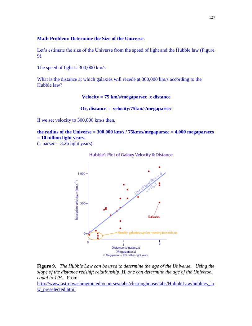
127

Math Problem: Determine the Size of the Universe.

Let’s estimate the size of the Universe from the speed of light and the Hubble law (Figure

9).

The speed of light is 300,000 km/s.

What is the distance at which galaxies will recede at 300,000 km/s according to the

Hubble law?

Velocity = 75 km/s/megaparsec x distance

Or, distance = velocity/75km/s/megaparsec

If we set velocity to 300,000 km/s then,

the radius of the Universe = 300,000 km/s / 75km/s/megaparsec = 4,000 megaparsecs

= 10 billion light years.

(1 parsec = 3.26 light years)

Figure 9. The Hubble Law can be used to determine the age of the Universe. Using the

slope of the distance redshift relationship, H, one can determine the age of the Universe,

equal to 1/H. From

http://www.astro.washington.edu/courses/labs/clearinghouse/labs/HubbleLaw/hubbles_la

w_preselected.html

128

It is possible to view the Universe as a potential black hole. Remember that a black hole

is simply a region with enough density to curve space sufficiently to prevent any light or

matter from leaving the confines of the black hole. But this is exactly how we are talking

about our expanding Universe if it exceeds its critical density, the curvature of all space

would be high enough to contain all light and matter. Using the approximation of 10

billion light years for the size of the Universe, one can use this as the Schwarzschild

radius of the Universe to calculate what density the Universe must exceed to be a black

hole. It turns out that this is the same as the critical density for a bound Universe, and is

10-30

grams per cubic centimeter or roughly three hydrogen atoms per cubic meter. But

wait one minute! If we are in a black hole why aren’t we crushed into some singularity?

If the Universe has a density greater than the critical density it will eventually contract

upon itself, forming a singularity. But this will take an enormous length of time, perhaps

100s of billions of years. If the mass density of the Universe exceeds its critical density,

we know that the Universe cannot ever expand outside its Schwarzschild radius. We may

be living inside a black hole Universe which itself contains black holes.

WebVideo: Recent Results from WMAP

http://www.youtube.com/watch?v=a7hizlLWZrY

Summary

In the infinitesimal slice of time after the Big Bang, from t = 0 to 10-43

seconds, there was

only a single unified force. At t = 10-12

seconds, this single force had separated into the

four known forces: gravity, electrical force, strong force, and weak force. Prior to 10-6

s

matter existed only as individual quarks; subsequently the Universe was cool enough for

quarks to stick together as individual protons and neutrons. During the 1st second, matter

and antimatter were created from high-energy gamma rays in nearly equal amounts.

During the first 3 minutes atomic nuclei were formed, including hydrogen, helium, and

lithium. For the first 300,000 years the Universe was dominated by radiation and was

opaque to light. Subsequently the Universe cooled enough to form neutral atomic

hydrogen (a proton orbited by an electron) which is transparent to light. After this

decoupling of matter and radiation, matter was clumped by gravity.

The near-isotropy of the cosmic fireball radiation is explained by a sudden inflation in the

size of the Universe between 10-35

s and 10-33

s.

The future of the Universe is determined by whether or not the Universe exceeds the

critical mass density. If its density is smaller, then we live in an open Universe. If its

density is larger, we live in a closed Universe. We do not know whether the measured

mass density of the Universe is smaller or larger than this critical density. One test that

can be made is to examine the Hubble law for curvature at high red shifts. The distance

determination of high red shift galaxies is not yet accurate enough to make a reliable

determination.

129

Key Words & Phrases

1. antimatter – each particle of matter has an antimatter equivalent, when the two

collide they annihilate each other producing energy

2. critical density – a mass density of the Universe, above which the Universe is open,

below which it is closed

3. dark matter – unknown matter that makes up to 90% of a galaxies mass

4. deuterium – hydrogen with a nucleus of one proton and one neutron

5. inflation – the abrupt increase in size of the Universe at the beginning of the Big

Bang

6. Grand Unified Theory – a unified force theory in which under conditions of high-

temperature all four forces are indistinguishable and behave as one

7. Pair production – the production of a particle of matter and its corresponding

antimatter particle from the collision of two high-energy gamma ray photons

8. Planck time – the time interval immediately after the Big Bang, during which there

was only one force

9. Tritium – a hydrogen atom with one proton and two neutrons

Review for Understanding

1. How does the distance-red shift relation tell us whether the Universe is open or

closed?

2. How is matter thought to have been formed in the Big Bang? How has this been

tested?

3. Discuss the critical density of the Universe. Is it exceeded?

Essay Questions

1. If the Universe is open, what will eventually happen to the cosmic background

radiation? If it is closed, what will happen to it?

2. Why is determining the abundance of helium and lithium in older stars so important?

3. How can the Universe be compared with a black hole?

4. Our Solar System contains significant quantities of heavy elements. If the Universe

were formed in a Big Bang, which produced only hydrogen and helium, what can we

conclude about the age and history of the Solar System? Is the Solar System as old

as the Universe?

Figure 5. A baseball thrown high in the air is analogous to a bound Universe. Original.

130

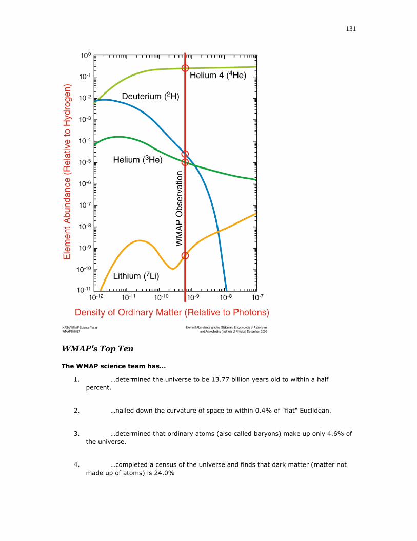
131

WMAP's Top Ten

The WMAP science team has…

1. …determined the universe to be 13.77 billion years old to within a half

percent.

2. …nailed down the curvature of space to within 0.4% of "flat" Euclidean.

3. …determined that ordinary atoms (also called baryons) make up only 4.6% of

the universe.

4. …completed a census of the universe and finds that dark matter (matter not

made up of atoms) is 24.0%

132

5. …determined that dark energy, in the form of a cosmological constant, makes

up 71.4% of the universe, causing the expansion rate of the universe to speed

up. - "Lingering doubts about the existence of dark energy and the

composition of the universe dissolved when the WMAP satellite took the most

detailed picture ever of the cosmic microwave background (CMB)." -

http://map.gsfc.nasa.gov/media/ContentMedia/A2218.jpg

133

________________________________________________________________________

Chapter 28 – Origin and Evolution of Life: on Earth

and Elsewhere ________________________________________________________________________

We shall not cease from exploration.

And the end of all our exploring.

Will be to arrive where we started.

And know the place for the first time.

-- T.S. Eliot

To see a world in a grain of sand,

And heaven in a wild flower:

Hold infinity in the palm of your hand,

And eternity in an hour.

--Blake, Auguries of Innocence (1757-1827)

Chapter Preview

In the first 27 chapters of this text we have reviewed the arguments for humans not

occupying a central place in the Universe. Historically, scientists discovered that the

Earth is not at the center of the Solar System, the Sun is not at the center of the Milky

Way, and the Milky Way is not at the center of the Universe, any more than any other

galaxy. We now need to ask ourselves the question, “Are we the only example of

intelligent life in our galaxy?” One of the most risky but potentially rewarding studies in

modern science is the search for extraterrestrial intelligence and the attempted

communication with other life forms. This is an area of study bordering on biology and

astronomy. In this chapter we will briefly review the origin and evolution of life on Earth

and evaluate the chances for the existence of intelligent life elsewhere in the Milky Way.

Key Physical Concepts to Understand: definition of life, evolution of primitive life on

Earth, the Drake equation, SETI

I. Introduction

Humans have had a tendency to feel that the Earth is a special place in the Universe,

perhaps for no good reason, from ancient times until the present. From the time of the

Copernican revolution in 1510, when the Earth was displaced by the Sun as the center of

the Solar System, humans have become increasingly aware that we are not in a revered

place. Now scientists have come to understand that man has no central role in the

134

Universe. This is called the Principle of Mediocrity, a principle that was resisted by

entrenched theology in the time of Copernicus. But more recent philosophical/physical

inquiry suprisingly leads counter to the Principle of Mediocrity and has resulted in the

following Anthropic Principle: Without intelligent life, the Universe is meaningless,

for there is no one to study or contemplate its existence. This is not a mere

unsupported philosophical statement. Recent physical/cosmological coincidences have

been pointed out by a number of physicists (WebEssay: The Anthropic Principle),

including Brandon Carter, John Wheeler, Richard Gott, and Robert Dicke. The existence

of life in our Universe appears to be the result of a delicate balance in the strength of

gravity, the strong force, and the expansion rate of the Universe. A slight change in any

one of these physical parameters would eliminate any chance of life in our Universe. The

fact that we are alive in the 20th

century constrains some of the most basic physical laws.

There is a deep connection between particle physics, cosmology, and the origin of life.

One of the most fundamental questions in science is: “Are we unique and alone, or are we

the result of the natural and relentless evolution of countless life-forms in a fertile

Universe?” In this chapter we will all too briefly examine the probability for intelligent

life elsewhere in our galaxy. First we must agree on a basic definition for life. Then we

must examine the scarce clues that nature has provided us to estimate the probability of

finding life elsewhere.

WebVideo: Why are we here?

http://www.youtube.com/watch?v=EUe_Vfi5IL0&feature=related

II. What is Life?

What is life? Oddly enough, there is no clear, widely agreed upon definition of life. We

know it when we see it, but how do we make the classification? One way of constructing

a definition is to make a list of properties of life and then review it to determine how

adequately one can use these properties to define it.

The Russian philosopher Alexander Koyre observed: “What is life? – this question

concerns us all and is one of the most important in cosmology. We divide the world into

living and nonliving things but still have no widely accepted meaning of the word life.

Complex organisms are composed of cells, which are composed of molecules, which are

composed of atoms; and it is not clear at what level of complexity life first emerges. The

cell is a miracle of the physical world and required billions of years to evolve; dare we

exclude it assert that it is nonliving, and claim that life is manifest only in complex multi-

cellular organisms?

“Living organisms feed, grow, move, reproduce, and behave in response to their

environment. Many things admittedly non-living exhibit similar properties. An

automobile moves and consumes food; a crystal grows; a candle flame needs

nourishment, reacts to its environment, and self-reproduces with sometimes alarming

consequences. Manmade automatons are extremely intricate, and computers now play

chess with each other. With so many nonliving things mimicking the characteristics

135

usually ascribed to organisms, it is difficult to pinpoint exactly what defines life. Are we

to believe that self-reproduction and evolution are the hallmarks of life? According to

biochemistry, self-reproduction is possible in highly organized chemical systems, and

according to biology, evolution operates automatically by means of natural selection.

The physical world, it seems, has an astonishing power for creating organized

complexity, and there is nothing of a physical nature that sets life apart from the rest of

the physical world.”

Life on Earth is based on complex carbon molecules, which can form gigantic molecules

containing millions of atoms. No other element comes close to forming molecules with

the diversity and complexity that carbon can form. The carbon compounds containing

one or more carbon-hydrogen bonds are called organic molecules, even if they are not

found in living organisms. Other important elements in the compounds found in living

systems are nitrogen, oxygen, sulfur, and phosphorus; all are formed via fusion in stellar

cores. Life, or at least life as we know it on Earth, is based on complex self-reproducing

organic molecules, DNA in particular (Figure 1). DNA is a long chain-like molecule that

can split and then each half can attract new atoms so it can rebuild the whole, thus

reproducing itself. DNA stores information in terms of molecular sequences on its chain

structure, genetic information used to construct a complete organism. Although the DNA

in an oak tree, a toad, and a person are so similar that they indicate a common ancestry,

yet the detailed differences in the DNA structure make an oak tree different from a

person.

Figure 1. Model of the structure of DNA.

Amino acids are relatively simple organic molecules, which form a basic building block

to build protein molecules, which link in different shapes and structures (Figure 2).

Proteins are used in living organisms to build cell walls, and as enzymes to catalyze

chemical reactions necessary for life. Cells are in turn organized into entire organisms.

136

Figure 2. Schematic of amino acids and proteins.

Our first clue in being able to estimate (or guess) the probability of finding intelligent life

elsewhere in the Universe…

Clue A: The characteristics of the simplest forms of life on Earth.

III. The Miller-Urey Experiment

Is there evidence that the biochemical processes that occurred in the evolution on

Earth occur naturally, that is could they occur again, even on another planet? In the

1950s, American chemists Stanley Miller and Harold Urey performed a chemical

simulation of the primitive Earth (Figure 3). They constructed a closed container in the

laboratory, which contained hydrogen, methane, and ammonia gases, along with water,

which they thought best represented the composition of the Earth’s oceans and

atmosphere. Through this mixture Miller and Urey passed electrical sparks, analogous to

the lightning that must have zapped the early Earth. After several days Miller and Urey

stopped their experiment and analyzed their container. They found an organic muck rich

in amino acids. This experiment has been repeated many times using different

137

compounds to represent the early atmosphere and different energy sources, ultraviolet

radiation for example; amino acids are always created.

Figure 3. A schematic diagram of the Miller Urey experiment. In the 1950s this

experiment showed that amino acids, one of the chemical building blocks of life, could

easily be produced in an environment similar to the primitive Earth. FMW 589-E.4

Modified.

It should be emphasized that neither Miller and Urey nor anyone since has created life in

a test tube. The significance of their experiment is that they showed how a simple

chemical building block for life could be expected to naturally evolve in the environment

provided by the primitive Earth. How life evolved from amino acids to single-celled

organisms is still a mystery.

Clue B: The natural process of formation of amino acids on Earth.

Chapter ?? Section ?? discussed the discovery of amino acids in meteorites found on the

Earth. Sri Lankan meteorite chemist Cyril Ponnamperuma discovered all of the basic

molecules coding genetic information in DNA in a single carbonaceous chondrite, but no

life. This provides a vivid illustration that the amino acid building blocks used by all

organisms on Earth are even synthesized in interstellar space. Emission from molecules

of the amino acid glycine floating free in interstellar space have even been detected by

radio astronomers. Amino acid molecules have also been found on some primitive

meteorites. The Miller Urey experiment gives us a tantalizing hint that live could easily

138

have evolved elsewhere in the Universe, given a physically and chemically friendly

environment.

Clue C: The discovery of organic compounds in space.

V. What Conditions are Necessary for Life?

We know that the Earth has the conditions necessary for life, and from that we can make

some assumptions. Life on Earth is dependent on the existence of liquid water, solar

energy that keeps a stable temperature that is neither so cold nor so hot that water can’t

exist on the surface in liquid form. It also required that the temperature of the

environment remains stable long enough, billions of years, for life to evolve. In other

words, it is generally accepted that the formation of life on a planet requires a stable

temperate climate – not so cold that water is frozen or so hot that liquid water doesn’t

exist. In addition a planet support life requires and an environment shielded from the

sterilizing effects of ultraviolet radiation.

A main sequence star that has a main sequence lifetime of several billion years or more

and provides enough warmth to one or more planets would be a logical candidate for

life. If the planets are too close to the mother star, or too far, water would either in a

frozen state or would have been vaporized. A high mass star isn’t a likely candidate for

the evolution of life, as it would have a short life span on the main sequence. However,

if a star has an extremely low mass, and therefore low luminosity, it still might have a

planet close enough to warm the surface to an Earth-like temperature, but at such a small

distance from the central star, a planet would have a rotational period tidally locked to

it’s period of revolution, making days unbearably long and hot, and nights unbearably

long and cold, similar to Mercury. This leads to the “Goldilocks effect,” the formation

of life requires a star not too massive or too small, and a planet at a distance not too

large or two small. In addition, a planet has to be large enough to have sufficient

gravity to retain a protective atmosphere, but not so large to be a Jovian planet with no

solid surface.

There are a number of planets that have the characteristics required for habitability,

Earth-sized planets orbiting solar-like stars at a distance rendering them viable for the

evolution of life.

Clue D: The discovery of extrasolar planets, especially Earth-like planets.

139

Figure 4. Discovery of extrasolar planets by the Kepler mission. Plotted are the

discoveries (color coded by date of discovery) showing planet size (with respect to the

Earth) vs. expected temperature of the planet surface (assuming no greenhouse effect).

The left-most and right-most dashed lines represent the temperature limits of the

habitable zone while the center dashed line represents the Earth’s ambient temperature.

From http://astrobites.org/2012/02/29/keplers-habitable-worlds/

Figure 5. Exoplanets that are viable candidates for the formation of life are found in a

“habitable zone,” within a range of heliocentric distance depending on the mass of the

central star. From http://www.weirdwarp.com/2009/08/defining-alien-life-the-

different-weird-forms-et-could-take/

140

WebVideo: The Search for Habitable Planets

http://www.youtube.com/watch?v=vSKAccC_mOQ

VI. Primitive Life on Earth

From the Miller Urey experiment we can infer that the building blocks for life on Earth

are simple molecules of two types, amino acids and nucleotides. These molecules are

made from carbon, nitrogen, oxygen, and a tiny abundance of other elements. Amino

acids are joined together in living organisms into chains called proteins. Nucleotides are

similarly joined to form the molecular chains of the nucleic acids DNA and RNA, found

in the nuclei of cells. DNA is the long molecule with the structure of a double helix that

carries the genetic information of a cell.

The concept of a living cell was introduced in 1665 by the English scientist Robert

Hooke. The word cell comes from the Latin word cella, for small room

(http://www.etymonline.com/index.php?term=cell ). Hooke used the term, for the first

time, in a biological context, to describe observations of plant tissue through a

microscope, as they reminded him of a monk’s cell. The theory that all organisms are

built from cells was proposed in the 19th

century. Single celled organisms vary from

small bacteria with diameters only hundreds of times the diameter of the hydrogen atom

to the yolk of six-inch ostrich eggs (Figure 4). Multicellular organisms contain

interacting cells of differing function which depend upon each other for survival.

Humans have roughly 1014

cells each of which contains 1014

atoms.

Figure 6. Among the largest and smallest of individual calls – an ostrich egg and a

bacterium. From pective.com and Barcroft/Fame Pictures

There are basically two kinds of cells, prokaryotes and eukaryotes. The first single-

celled organisms to evolve were the prokaryotes, also the simplest organisms. Eukaryotes

evolved later and are considerably more complex. A prokaryote is characterized by the

absence of a cell nucleus; DNA is dispersed throughout the cell. A eukaryote has its

DNA in a small region within the cell called the nucleus.

In the 20th

Century all life was divided into two kingdoms the plant and animal kingdoms.

Now most biologists classify life forms into five kingdoms:

141

monera (bacteria and blue-green algae, all are prokaryotes),

portista (diatoms, amoeba, seaweed, and slime molds),

fungi (including yeast),

planate – common plants, and

animalia all eukaryotes, including humans.

Living organisms can be classified into two basic types according to the way they obtain

energy: autotrophs and heterotrophs. Autotrophs, including plants and algae, are self-

nourished; their food is the inorganic chemicals that they consume. Their energy usually

comes from sunlight via photosynthesis, in which carbon dioxide and water and sunlight

are converted to sugars and oxygen. Chemical energy is stored in sugars. Blue-green

algae are the first life forms to appear in the fossil record, and are found in rocks 3.5

billion years old (Figure 7).

How cells originated and evolved is not known but a likely picture of their origin can be

built through educated speculation. The first cells may have been primitive bacteria

heterotrophs that consumed organic molecules and derived their energy directly from

them. As number of primitive heterotrophs rapidly increased the supply of organic

chemical “food” on Earth dwindled. With the decline of simple chemical food sources,

any simple autotrophs that developed would have an advantage and would increase in

population at the same time that the homotrophs became decimated.

Figure 7. Fossils of blue-green algae, cyanobacteria. Above are individual fossilized

cells; below is a stromatolite, a layered, fossilized structure formed from biofilm of

142

cyanobacteria. From http://www.astrobio.net/exclusive/3636/stepping-stones-through-

time

Clue E: The fossil record of evolution of life on Earth indicates that nearly 1 billion years

were necessary for the appearance of life.

Toward end of the proterozoic era (2.5 billion to 500 million years ago) the highest

forms of life were the single-celled eukaryotes. The evolving atmosphere of the Earth

was becoming friendlier to life, e.g. the ozone layer protected the Earth’s surface from

destructive ultraviolet radiation. With this new found protection eukaryotes were able to

evolve into a multitude of multi-cellular organisms. A variety of invertebrates appeared

in the fossil record in a hundred million years or so, with an explosion of the number of

vertebrate and plant species following. A compressed timeline of the evolution of

lifeforms on earth is shown in Figure 8.

Figure 8. Timeline of the development of life forms on Earth. From Wikimedia

commons.

143

IIX. The Theory of Biological Evolution

The modern theory of biological evolution was proposed independently by the English

naturalists Charles Darwin and Alfred Wallace in 1858. Darwin has received most of the

credit based on his famous book “Origin of the Species”. Evolution is based on the ideas

that organisms in a single species differ by small amounts. Sometimes these small

differences allow some individuals to adapt better to the environment than others. The

environment continually stresses individual organisms. Those that have an edge will live

longer and produce more offspring than the more poorly adapted. Offspring will in turn

preferentially inherit those traits that are beneficial to survival. The environment favors

some inherited traits and disfavors others. Disfavored traits will then tend to be lost in

successive generations, while favored traits will tend to represent more and more

individuals in the entire population. This process is called natural selection.

One of the classic examples of evolution is that of the peppered moth

(http://en.wikipedia.org/wiki/Peppered_moth_evolution). Over the last 200 years the

peppered moth has changed its appearance to adapt to its environment. In pre-industrial

England the predominant variety of the peppered moth had a salt-and-pepper coloration in

keeping with its name. This served the moth well, as it was camouflaged whenever it

rested on the surface of lichen-covered trees with light bark. During the industrial

revolution, pollution from coal burning killed lichens and covered trees with soot. The

lightly colored moths died out, as they became more visible to predators, and were largely

replaced by the dark colored variety which became more successful. With the attenuation

of pollution in Britain in recent times, the lighter peppered moth has flourished once

again.

The theory of evolution proposed by Darwin and Wallace did not explain the mechanism

of inheritance of traits or the origin of individual differences. Traits are inherited through

the genetic code of DNA that carries traits from generation to generation through the

chemical self-replication of DNA. Mutations are changes in the DNA which happen

when the DNA is chemically or physically transformed, e.g. as a result of intense

exposure to radiation, or through a slip in the self-reproduction process.

WebVideos: Some Genetic Evidence for Evolution

http://www.youtube.com/watch?v=5saKcgnswA4

http://www.youtube.com/watch?v=urthr04mqoI

IX. The Drake Equation: Life in Other Star Systems?

How can we estimate the probability for life elsewhere in the Universe? Now we can

combine our clues to guess the probability of finding intelligent life anywhere else in the

Milky Way.

The Drake equation, formulated in 1961 by the American radio astronomer Frank Drake,

provides an estimate of the number of extrasolar civilizations in the Milky Way galaxy:

144

Equation 28.1: N = R fp ne fl fI fc L,

where

R is the rate at which solar-type stars form,

fp is the fraction of stars with planets,

N is the number of planets per star system suitable for life,

fl is the fraction of planets suitable for life where life actually arises,

fi is the fraction life-bearing planets where evolution to intelligent life occurs,

fc is the fraction of planets with intelligent life that develop a communications

technology and choose to use it for the search for extraterrestrial intelligence, and

L is the expected lifetime of such a civilization.

The Drake equation presents the number of civilizations that we could possibly

communicate with as a product of terms that we can estimate.

Table 28.1: Estimates of the Number of Detectable Civilizations from the Drake

Equation

Factor Lower Estimate Higher Estimate

R 1 per year 1 per year

fp 0.5 0.5

N 0.01 0.1

fl 1 1

fi 0.1 1

fc 1 1

L 100 years 1 million years

Number 0.05 50,000

R, the rate of formation of stars with properties friendly to the evolution of life. Since life

originated 3.5 to 4 billion years ago on the Earth, we can speculate that it would take life

3 to 4 billion years to evolve on any planet in the galaxy. Armed with only one example

of the occurrence of life on a planet we can assume nothing else. If this assumption is

correct it would be useless to search for intelligent life on any planet orbiting a star that is

so massive that it will not live for at least 3 billion years. We would expect intelligent

life-bearing planets to exist in orbit about mid-mass main sequence stars like the Sun.

Statistical studies of stars the Milky Way estimate that one such star forms in our galaxy

each year.

fp, the fraction of stars that form planets. Many think that all non-multiple star systems

form planets. An estimate of the number of stars without stellar companions is roughly

0.5 (Chapter xxx).

145

N, the average number of environmentally habitable planets orbiting stars that have

planets. The rest of the factors in the Drake equation are uncertain at best. The mean

number of planets that have an environment suitable for the evolution of life orbiting stars

that have planets is one if we use the number of planets that we know are hospitable to

the formation of life in our own Solar System. A planet must be far enough from the Sun

that the Sun’s energy doesn’t boil off the planet’s atmosphere or destroy life with

blistering heat. At the same time a planet can’t be so far away from its central star that it

receives to little life-giving warmth to support life. N could be 1 from our own

experience, or much less, say 0.1, if we want to make a conservative estimate.

It is hard to estimate fl , fI , and fc, but we know they can’t be greater than 1. Lets choose fl

= 1, fI = 0.1, and fc = 1 for a conservative estimate, and fl = 1, fI = 1, and fc = 1 for an

optimistic one. The expected lifetime of an intelligent civilization cannot be estimated

with any degree of reliability. We don’t know whether intelligent life on Earth will be

limited to a 100-year period by weapons of mass destruction, pollution, famine, and

disease or whether we as humans will learn from our mistakes before it is too late.

Estimates could legitimately range from 100 years to many millions of years. Let’s take

L=100 years as a pessimistic estimate and 1 million years as an optimistic estimate.

The resulting pessimistic and optimistic estimates for the total number of intelligent

civilizations in our galaxy with which we could communicate is much less than one to

one million. Our conclusion is that we have no idea whether there are any other

civilizations in the Milky Way that we could communicate with, or countless numbers of

such civilizations. We can only attempt such communications. What about

civilizations in other galaxies? The existence of such civilizations is academic, for the

time required to send them a communication at the speed of light and await a return

answer would be a minimum of millions of years, perhaps longer than our own

civilization will last.

X. The Search for Intelligent Life on Other Planets

How do we search for extraterrestrial civilizations? How would they choose to

communicate with us? The use of electromagnetic radiation is the logical choice.

Humans already use radio waves for communication on Earth. Light is the fastest means

of communication known; it can travel at the speed of light. Radio waves in particular

are an optimum means for communicating across interstellar space, as they easily

penetrate dust and gas.

If we agree that radio waves are the logical choice for communication, how to we choose

which frequencies to listen to? We assume that aliens would use the same criteria as we

would. We would choose a clear frequency with as little interference as possible. A band

of relatively noise-free frequencies exists in the microwave region of the spectrum. 21

centimeters is also a good choice because astronomers build large radio dishes for

measurements at 21-cm telescopes to study the distribution of hydrogen atoms in space.

146

We currently have the technology to detect extraterrestrial communications, and have had

it for several decades. One of 1st searches for extraterrestrial intelligence, abbreviated

SETI, was made in 1960 by Frank Drake who used radio telescopes to monitor nearby

solar stars for radio transmissions.

NASA and private funding have continued the SETI work into the 1990s using computers

and radio telescopes in an all-sky survey examining hundreds of stars over a range of

radio frequencies. The largest radio telescopes, including the 1000-m ? Arecibo radio

telescope have been used to monitor tens of millions of radio frequencies simultaneously

(Figure 7). What is the motivation for us as a society to spend tax dollars on SETI?

An extraterrestrial contact would be one of the greatest events in human history. The

scientific discoveries that would be communicated to us in a short period of time could be

enormously profound causing a quantum leap in technological development. The impact

of society would have unprecedented impact on our culture in ways that we can’t predict.

Figure 7. The Arecibo 1000-foot diameter radio telescope in Puerto Rico. Arecibo is the

largest telescope on Earth. Schweiker, NOAO.

We have been sending radio and television communications into space for the last 75

years. Are other intelligent civilizations monitoring us for signs of life? Would they

reply? Would they even recognize us as intelligent after receiving decades of sit-com

transmissions and reality television? Will our descendants be here to receive

transmissions in another 100 years?

147

WebVideos (Very Good): The Drake Equation and the Search for Life

1. http://www.youtube.com/watch?v=JnnEeRZqpYs&list=PL7D2535E668B41050

2. http://www.youtube.com/watch?v=iSRuxMnQeCY&list=PL7D2535E668B41050

3. http://www.youtube.com/watch?v=EgEMzPWU3ks&list=PL7D2535E668B4105

0

4. http://www.youtube.com/watch?v=phyYP4z6EyU&list=PL7D2535E668B41050

5. http://www.youtube.com/watch?v=prFKue_bTY4&list=PL7D2535E668B41050

6. http://www.youtube.com/watch?v=QEIdAkK-XFs&list=PL7D2535E668B41050

WebNote: The Anthropic Principle

anthrop.htm

http://en.wikipedia.org/wiki/Anthropic_principle

WebVideo: Fine Tuning and Multiverses

http://www.youtube.com/watch?v=2cT4zZIHR3s (Susskind)

http://www.youtube.com/watch?v=bf7BXwVeyWw (TED)

Summary

Key Words & Phrases

1. Amino acid

2. Autotroph

3. DNA

4. Drake equation – the equation that estimates the number of intelligent civilizations

in the Milky Way with which it is possible to communicate

5. Eukaryote – cells with DNA in nuclei

6. heterotroph

7. natural selection – the process in the theory of evolution in which organisms with

favorable inherited traits reproduce with more abundance that those with unfavorable

inherited traits

8. nucleotide

9. prokaryote – cells with no nuclei, instead DNA is spread throughout the cell’s

interior

10. protein

11. SETI – an abbreviation for Search for Extraterrestrial Intelligence

Review for Understanding

1.

Essay Questions

1.

148