chapter 22csd.newcastle.edu.au/book_slds_download/ch22c.pdf · chapter 22 © goodwin, graebe,...
TRANSCRIPT

© Goodwin, Graebe, Salgado , Prentice Hall 2000Chapter 22
Chapter 22
Design via Optimal ControlDesign via Optimal ControlTechniquesTechniques

© Goodwin, Graebe, Salgado , Prentice Hall 2000Chapter 22
In the author’s experience, industrial control systemdesign problems can be divided into four categories:1. Relatively simple loops for which PID design gives a
very satisfactory solution (see Chapters 6 and 7).
2. Slightly more complex problems where an additional feature beyond PID yields significant performance advantages. Two key tools that can be used to considerably advantage in this context are feedforward control (Chapter 10) and the Smith Predictor for plants with significant time delays (Chapters 7 and 15).

© Goodwin, Graebe, Salgado , Prentice Hall 2000Chapter 22
3. Systems involving significant interactions but where some form of preliminary compensation essential converts the problem into separate non-interacting loops which then fall under categories 1 and 2 above (Chapter 21).
4. Difficult problems which require some form of computer assisted optimization for their solution. (This is the topic of the current chapter and Chapter 23).

© Goodwin, Graebe, Salgado , Prentice Hall 2000Chapter 22
As a rough guideline: 95% of control problems fallinto category 1 above; 4% fall into category 2 or 3.The remaining 1% fall into category 4.
However, the relative low frequency of occurrence ofthe problems in category 4 is not representative oftheir importance. Indeed, it is often this 1% of hardproblems where the real benefits of control systemdesign can be achieved. They are often the make orbreak problems.

© Goodwin, Graebe, Salgado , Prentice Hall 2000Chapter 22
We will emphasize methods for solving thesetougher problems based on optimal control theory.There are three reasons for this choice:1. It is relatively easy to understand
2. It has been used in a myriad of applications. (Indeed, theauthors have used these methods on approximately 20 industrial applications).
3. It is a valuable precursor to other advanced methods - e.g., Model Predictive Control, which is explained in thenext chapter.

© Goodwin, Graebe, Salgado , Prentice Hall 2000Chapter 22
The analysis presented in this chapter builds on theresults in Chapter 18, where state space designmethods were briefly described in the SISO context.We recall, from that chapter, that the two keyelements were
◆ state estimation by an observer◆ state-estimate feedback

© Goodwin, Graebe, Salgado , Prentice Hall 2000Chapter 22
State-Estimate Feedback
Consider the following MIMO state space modelhaving m inputs and p outputs.
By analogy with state-estimate feedback in the SISOcase (as in Chapter 7), we seek a matrix K ∈ �m×n anda matrix J ∈ �n×p such that (Ao - BoK) and (Ao - JCo)have their eigenvalues in the LHP. Further we willtypically require that the closed-loop poles reside insome specified region in the left-half plane. Tools suchas MATLAB provide solutions to these problems.
x(t) = Aox(t) + Bou(t)y(t) = Cox(t)

© Goodwin, Graebe, Salgado , Prentice Hall 2000Chapter 22
Example 22.1
Consider a MIMO plant having the nominal model
Say that the plant has step-type input disturbances inboth channels.
Using state-estimate feedback ideas, design amultivariable controller which stabilizes the plantand, at the same time, ensures zero steady-state errorfor constant references and disturbances.
Go(s) =1
s(s+ 1)(s+ 2)
[2(s+ 1) −0.5s(s+ 1)
s 2s
]

© Goodwin, Graebe, Salgado , Prentice Hall 2000Chapter 22
We first build state space models (Ap, Bp, Cp, 0) and(Ad, Bd, Cd, 0) for the plant and for the inputdisturbances, respectively.
We estimate not only the plant state xp(t) but also thedisturbance vector di(t). We then form the controllaw
u(t) = −Kpx(t)− di(t) + r(t)

© Goodwin, Graebe, Salgado , Prentice Hall 2000Chapter 22
One pair of possible state space models is
where
and
xp(t) = Apxp(t) + Bpu(t) y(t) = Cpxp(t)xd(t) = Adxd(t) + Bdu(t) di(t) = Cdxd(t)
Ap =
−3 −2 0 01 0 0 00 0 −2 20 0 0 0
; Bp =
1 20 00 −0.51 0
; Cp =
[0 0 1 00 1 0 0
]
Ad = 0; Bd = 0; Cd = I2

© Goodwin, Graebe, Salgado , Prentice Hall 2000Chapter 22
The augmented state space model, (A, B, C, 0) isthen given by
leading to a model with six states.
A =[Ap BpCd
0 Ad
]=[Ap Bp
0 0
]B =
[Bp
Bd
]=[Bp
0
]C =
[Cp 0
]

© Goodwin, Graebe, Salgado , Prentice Hall 2000Chapter 22
We then compute the observer gain J, choosing the sixobserver poles located at -5, -6, -7, -8, -9, -10. This isdone using the MATLAB command place for the pair(AT, CT).
Next we compute the feedback gain K. We note that it isequivalent (with ) to
i.e., we need only compute Kp. This is done by using theMATLAB command place for the pair (Ap, Bp). Thepoles in this case are chosen at -1.5 ± j1.32, -3 and -5.
0)( =tru(t) = −
[Kp Cd
] [xp(t)xd(t)
]=⇒ K =
[Kp I2
]

© Goodwin, Graebe, Salgado , Prentice Hall 2000Chapter 22
The design is evaluated by applying step referencesand input disturbances in both channels, as follows:
where di(1)(t) and di
(2)(t) are the first and secondcomponents of the input-disturbance vectorrespectively.
The results are shown on the next slide.
r1(t) = µ(t− 2); r2(t) = −µ(t− 5); d(1)i (t) = µ(t− 10); d
(2)i (t) = µ(t− 15)

© Goodwin, Graebe, Salgado , Prentice Hall 2000Chapter 22
Figure 22.1: MIMO design based in state-estimatefeedback
0 2 4 6 8 10 12 14 16 18 20−1.5
−1
−0.5
0
0.5
1
1.5
Time [s]
Pla
nt o
utpu
ts a
nd r
ef.
r1(t)
r2(t)
y1(t)
y2(t)
The above results indicate that the design is quitesatisfactory. Note that there is strong coupling butdecoupling was not part of the design specification.

© Goodwin, Graebe, Salgado , Prentice Hall 2000Chapter 22
We next turn to an alternative procedure that deals withthe MIMO case via optimization methods. Aparticularly nice approach for the design of K and J is touse quadratic optimization because it leads to simpleclosed-form solutions.

© Goodwin, Graebe, Salgado , Prentice Hall 2000Chapter 22
Dynamic Programming andOptimal Control
We begin at a relatively abstract nonlinear level butour ultimate aim is to apply these ideas to the linearcase.

© Goodwin, Graebe, Salgado , Prentice Hall 2000Chapter 22
The Optimal Control Problem
Consider a general nonlinear system with input u(t) ∈ �m,described in state space form by
Problem: (General optimal control problem). Find anoptimal input uo(t), for t ∈ [to, tf], such that
where ν(s, u, t) and g(x(tf)) are nonnegative functions.
uo(t) = argminu(t)
{∫ tf
to
V(x, u, t)dt+ g(x(tf ))}
dx(t)dt
= f(x(t), u(t), t)
© Goodwin, Graebe, Salgado , Prentice Hall 2000Chapter 22
Necessary Condition for Optimality
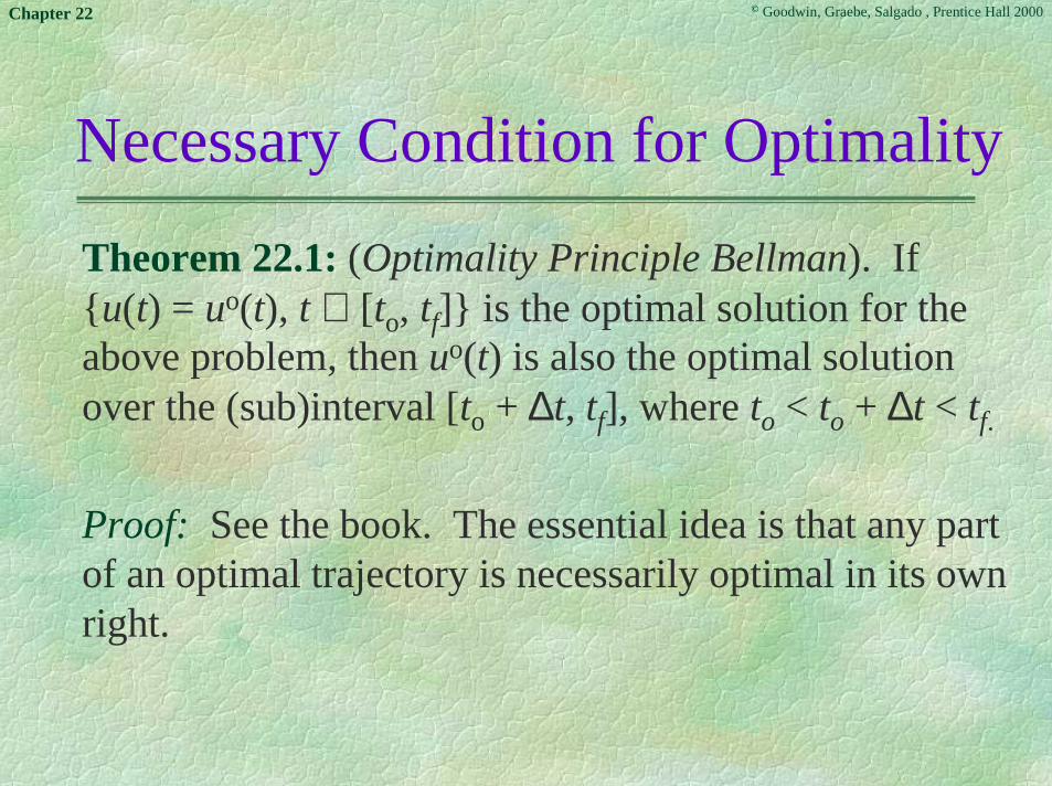
Theorem 22.1: (Optimality Principle Bellman). If{u(t) = uo(t), t ∈ [to, tf]} is the optimal solution for theabove problem, then uo(t) is also the optimal solutionover the (sub)interval [to + ∆t, tf], where to < to + ∆t < tf.
Proof: See the book. The essential idea is that any partof an optimal trajectory is necessarily optimal in its ownright.

© Goodwin, Graebe, Salgado , Prentice Hall 2000Chapter 22
We will next use the above theorem to derivenecessary conditions for the optimal u. The idea is toconsider a general time interval [t, tf], wheret ∈ [to, tf], and then to use the Optimality Principlewith an infinitesimal time interval [t, t + ∆t].
Some straightforward analysis leads to the followingequations for the optimal cost:

© Goodwin, Graebe, Salgado , Prentice Hall 2000Chapter 22
−∂Jo(x(t), t)∂t
= V(x(t),U , t) +[∂Jo(x(t), t)
∂x
]T
f(x(t),U , t)
The solution for this equation must satisfy the boundary condition
Jo(x(tf ), tf ) = g(x(tf ))

© Goodwin, Graebe, Salgado , Prentice Hall 2000Chapter 22
At this stage we cannot proceed further without beingmore specific about the nature of the originalproblem. We also note that we have implicitlyassumed that the function Jo(x(t), t) is well behaved,which means that it is continuous in its argumentsand that it can be expanded in a Taylor series.

© Goodwin, Graebe, Salgado , Prentice Hall 2000Chapter 22
The Linear Quadratic Regulator(LQR)
We next apply the above general theory to the followingproblem.
Problem: (The LQR problem). Consider a linear time-invariant system having a state space model, as definedbelow:
We aim to drive the initial state xo to the smallest possiblevalue as soon as possible in the interval [to, tf], butwithout spending too much control effort.
dx(t)dt
= Ax(t) + Bu(t) x(to) = xo
y(t) = Cx(t) + Du(t)
© Goodwin, Graebe, Salgado , Prentice Hall 2000Chapter 22
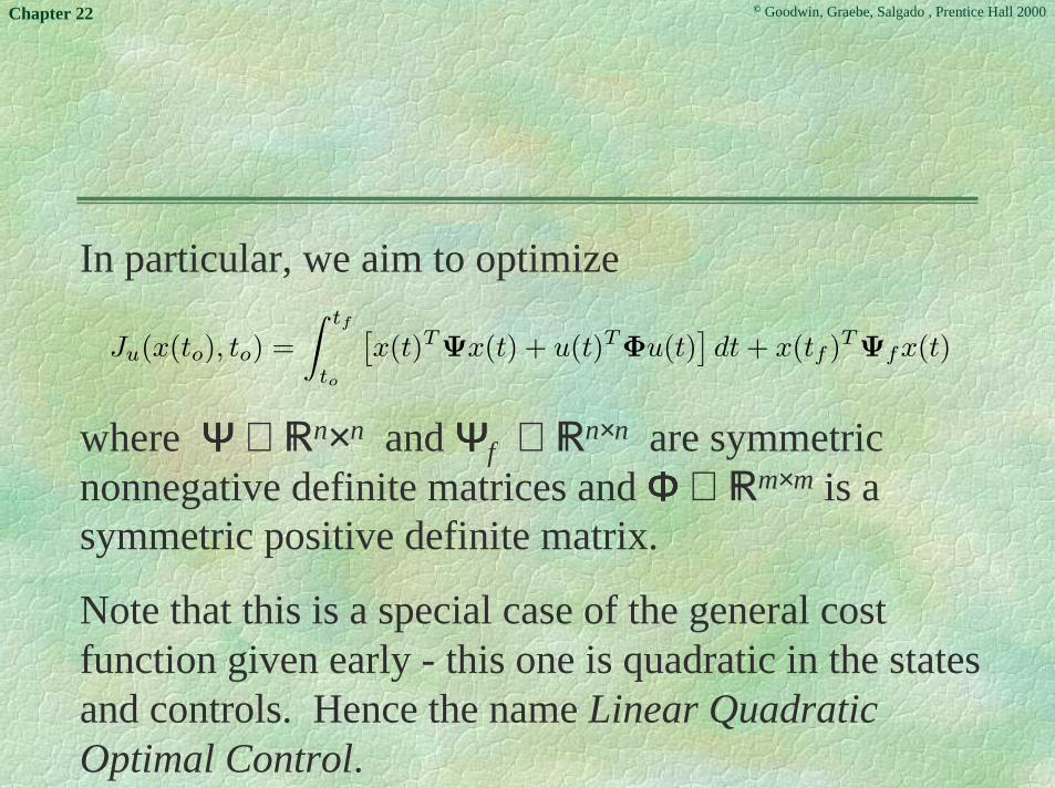
In particular, we aim to optimize
where ΨΨΨΨ ∈ �n×n and ΨΨΨΨf ∈ �n×n are symmetricnonnegative definite matrices and ΦΦΦΦ ∈ �m×m is asymmetric positive definite matrix.
Note that this is a special case of the general costfunction given early - this one is quadratic in the statesand controls. Hence the name Linear QuadraticOptimal Control.
Ju(x(to), to) =∫ tf
to
[x(t)TΨx(t) + u(t)TΦu(t)
]dt+ x(tf )TΨfx(t)

© Goodwin, Graebe, Salgado , Prentice Hall 2000Chapter 22
To solve this problem, the theory summarized abovecan be used. We first make the followingconnections between the general optimal problemand the LQR problem:
f(x(t), u(t), t) = Ax(t) + Bu(t)
V(x, u, t) = x(t)TΨx(t) + u(t)TΦu(t)
g(x(tf )) = x(tf )TΨfx(tf )

© Goodwin, Graebe, Salgado , Prentice Hall 2000Chapter 22
Simple application of the general conditions foroptimality leads to
where P(t) satisfies
uo(t) = −Ku(t)x(t)
where Ku(t) is a time varying gain, given by
Ku(t) = Φ−1BTP(t)
−dP(t)dt
= Ψ − P(t)BΦ−1BT P(t) + P(t)A + AT P(t)

© Goodwin, Graebe, Salgado , Prentice Hall 2000Chapter 22
The above equation is known as the Continuous TimeDynamic Riccati Equation (CTDRE). This equationhas to be solved backwards in time, to satisfy theboundary condition:
P(tf ) = Ψf

© Goodwin, Graebe, Salgado , Prentice Hall 2000Chapter 22
Some brief history of this equation is contained in theexcellent book:
Bittanti, Laub, Williams, “The Riccati Equation” ,Springer Verlag, 1991.
Some extracts are given below.

© Goodwin, Graebe, Salgado , Prentice Hall 2000Chapter 22
Some History of the Riccati Equation“Towards the turn of the seventeenth century, when the baroquewas giving way to the enlightenment, there lived in the Republicof Venice a gentleman, the father of nine children, by the nameof Jacopo Franceso Riccati. On the cold New Year’s Eve of1720, he wrote a letter to his friend Giovanni Rizzetti, where heproposed two new differential equations. In modern symbols,these equations can be written as follows.
Where m is a constant. This is probably the first documentwitnessing the early days of the Riccati Equation, an equationwhich was to become of paramount importance in the centuriesto come.”
22
2
ttxxtxx m
λβαβα
++=+=
�
�

© Goodwin, Graebe, Salgado , Prentice Hall 2000Chapter 22
Who was Riccati ?“Count Jacopo Riccati was born in Venice on May 28, 1676. Hisfather, a nobleman, died when he was only ten years old. The boywas raised by his mother, who did not marry again, and by apaternal uncle, who recognized unusual abilities in his nephew andpersuaded Jacopo Francesco’s mother to have him enter a Jesuitcollege in Brescia. Young Riccati enrolled at this college in 1687,probably with no intention of ever becoming a scientist. Indeed, atthe end of his studies at the college, in 1693, he enrolled at theuniversity of Padua as a student of law. However, following hisnatural inclination, he also attended classes in astronomy given byFather Stefano degli Angeli, a former pupil of BonaventuraCavalieri. Father Stefano was fond of Isaac Newton’sPhilosophiae Naturalis Principia, which he passed onto youngRiccati around 1695. This is probably the event which causedRiccati to turn from law to science.”

© Goodwin, Graebe, Salgado , Prentice Hall 2000Chapter 22
“After graduating on June 7, 1696, he married Elisabetta dei Contid’Onigo on October 15, 1696. She bore him 18 children, of whom 9survived childhood. Amongst them, Vincenzo (b.1707, d.1775), amathematical physicist, and Giordano (b.1709, d.1790) a scholarwith many talents but with a special interest for architecture andmusic, are worth mentioning.Riccati spent most of his life in Castelfranco Veneto, a little townlocated in the beautiful country region surrounding Venice. Besidestaking care of his family and his large estate, he was in charge of theadministration of Castelfranco Veneto, as Provveditore (Mayor) ofthat town, for nine years during the period 1698-1729. He alsoowned a house in the nearby town of Treviso, where he moved afterthe death of his wife (1749), and where his children had been usedto spending a good part of each year after 1747”.

© Goodwin, Graebe, Salgado , Prentice Hall 2000Chapter 22
Count Jacopo Franceso Riccati

© Goodwin, Graebe, Salgado , Prentice Hall 2000Chapter 22
Returning to the theory of Linear Quadratic OptimalControl, we note that the theory holds equally wellfor time-varying systems - i .e., when A, B, ΦΦΦΦ, ΨΨΨΨ areall functions of time. This follows since no explicit(or implicit) use of the time invariance of thesematrices was used in the derivation. However, in thetime-invariant case, one can say much more about theproperties of the solution. This is the subject of thenext section.
© Goodwin, Graebe, Salgado , Prentice Hall 2000Chapter 22
Properties of the Linear QuadraticOptimal Regulator
Here we assume that A, B, Φ, Ψ are all time-invariant. We will be particularly interested in whathappens at t → ∞. We will summarize the keyresults here.

© Goodwin, Graebe, Salgado , Prentice Hall 2000Chapter 22
Quick Review of Properties
We make the following simplifying assumptions:(i) The system (A, B) is stabilizable from u(t).
(ii) The system states are all adequately seen by the costfunction. Technically, this is stated as requiring that(ΨΨΨΨ½, A) be detectable.

© Goodwin, Graebe, Salgado , Prentice Hall 2000Chapter 22
Under these conditions, the solution to the CTDRE,P(t), converges to a steady-state limit Ps
∞ as tf → ∞.This limit has two key properties:❖ Ps
∞ is the only nonnegative solution of the matrix algebraic Riccati equation obtained by setting dP(t)/dt = 0 in
❖ When this steady-state value is used to generate a feedback control law, then the resulting closed-loop system is stable.
0 = Ψ − P∞BΦ−1BT P∞ + P∞A + AT P∞
−dP(t)dt
= Ψ − P(t)BΦ−1BT P(t) + P(t)A + AT P(t)

© Goodwin, Graebe, Salgado , Prentice Hall 2000Chapter 22
More Detailed Review of PropertiesLemma 22.1: If P(t) converges as tf → ∞, then the limitingvalue P∞ satisfies the following Continuous-Time AlgebraicRiccati Equation (CTARE):
The above algebraic equation can have many solutions.However, provided (A, B) is stabilizable and (A, ΨΨΨΨ½) hasno unobservable modes on the imaginary axis, then thereexists a unique positive semidefinite solution Ps
∞ to theCTARE having the property that the system matrix of theclosed-loop system, A - ΦΦΦΦ-1BTPs
∞, has all its eigenvalues inthe OLHP. We call this particular solution the stabilizingsolution of the CTARE. Other properties of the stabilizingsolution are as follows:
0 = Ψ − P∞BΦ−1BT P∞ + P∞A + AT P∞

© Goodwin, Graebe, Salgado , Prentice Hall 2000Chapter 22
(a) If (A, ΨΨΨΨ½) is detectable, the stabilizing solution is the onlynonnegative solution of the CTARE.
(b) If (A, ΨΨΨΨ½) has unobservable modes in the OLHP, then thestabilizing solution is not positive definite.
(c) If (A, ΨΨΨΨ½) has an unobservable pole outside the OLHP, then,in addition to the stabilizing solution, there exists at least oneother nonnegative solution to the CTARE. However, in thiscase, the stabilizing solution satisfies Ps
∞ -P∞ ≥ 0, where P∞is any other solution of the CTARE.
Proof: See the book.

© Goodwin, Graebe, Salgado , Prentice Hall 2000Chapter 22
Thus we see that the stabilizing solution of theCTRAE has the key property that, when this is usedto define a state variable feedback gain, then theresulting closed loop system is guaranteed stable.
We next study the convergence of the solutions of theCTRDE (a differential equation) to particularsolutions of the CTRAE (an algebraic equation).We will be particularly interested in those conditionswhich guarantee convergence to the stabilizingsolution.

© Goodwin, Graebe, Salgado , Prentice Hall 2000Chapter 22
Convergence of the solution of the CTDRE to thestabilizing solution of the CTARE is addressed in thefollowing lemma.Lemma 2.22: Provided that (A, B) is stabilizable, that(A, ΨΨΨΨ½) has no unobservable poles on the imaginaryaxis, and that the terminal condition satisfies: ΨΨΨΨf > Ps
∞,then
(If we strengthen the condition of ΨΨΨΨ to require that(A, ΨΨΨΨ½) is detectable, then ΨΨΨΨf ≥ 0 suffices).Proof: See the book.
limtf→∞
P(t) = Ps∞

© Goodwin, Graebe, Salgado , Prentice Hall 2000Chapter 22
Example
Consider the scalar system
and the cost function
The associated CTDRE is
and the CTARE is
x(t) = ax(t) + u(t)
J = ψfx(tf )2 +∫ tf
0
(ψx(t)2 + u(t)2
)dt
P (t) = −2aP (t) + P (t)2 − ψ; P (tf ) = ψf
(P s∞)2 − 2aP s
∞ − ψ = 0

© Goodwin, Graebe, Salgado , Prentice Hall 2000Chapter 22
Case 1: ψψψψ ≠≠≠≠ 0Here, (A, ΨΨΨΨ½) is completely observable (and thusdetectable). There is only one nonnegative solutionof the CTARE. This solution coincides with thestabilizing solution. Making the calculations, we findthat the only nonnegative solution of the CTARE is
leading to the following gain:
P s∞ =
2a+√
4a2 + 4ψ2
Ks∞ = a+
√a2 + ψ

© Goodwin, Graebe, Salgado , Prentice Hall 2000Chapter 22
The corresponding closed-loop pole is at
This is clearly in the LHP, verifying that the solutionis indeed the stabilizing solution.
Other cases are considered in the book.
pcl = −√a2 + ψ

© Goodwin, Graebe, Salgado , Prentice Hall 2000Chapter 22
To study the convergence of the solutions, we againconsider:
Case 1: ψψψψ ≠≠≠≠ 0Here (A, ΨΨΨΨ½) is completely observable. Then P(t)converges to Ps
∞ for any ψf ≥ 0.

© Goodwin, Graebe, Salgado , Prentice Hall 2000Chapter 22
Linear quadratic regulator theory is a powerful tool incontrol-system design. We illustrate its versatility inthe next section by using it to solve the so-called ModelMatching Problem (MMP).

© Goodwin, Graebe, Salgado , Prentice Hall 2000Chapter 22
Model Matching Based on LinearQuadratic Optimal Regulators
Many problems in control synthesis can be reducedto a problem of the following type:
Given two stable transfer functions M(s) and N(s), find a stable transfer function Γ(s) so that N(s)Γ(s) is close to M(s) in a quadratic norm sense.

© Goodwin, Graebe, Salgado , Prentice Hall 2000Chapter 22
When M(s) and N(s) are matrix transfer functions,we need to define a suitable norm to measurecloseness. By way of illustration, we consider amatrix A = [aij] ∈ �p×m for which we define theFröbenius norm as follows
||A||F =√traceAHA =
√√√√ m∑i=1
p∑j=1
|aij |2

© Goodwin, Graebe, Salgado , Prentice Hall 2000Chapter 22
Using this norm, a suitable synthesis criterion for theModel Matching Problem described earlier might be:
where
and where S is the class of stable transfer functions.
Γo = argminΓ∈S
JΓ
JΓ =12π
∫ ∞
−∞
∥∥M(jω)− N(jω)Γ(jω)∥∥2
Fdω

© Goodwin, Graebe, Salgado , Prentice Hall 2000Chapter 22
This problem can be converted into vector form byvectorizing M and ΓΓΓΓ. For example, say that ΓΓΓΓ isconstrained to be lower triangular and that M, N, andΓΓΓΓ are 3 × 3, 3 × 2, and 2 × 2 matrices, respectively;then we can write
where || ||2 denotes the usual Euclidean vector normand where, in this special case,
JΘ =12π
∫ ∞
−∞
∥∥V(jω)− W(jω)Θ(jω)∥∥2
2dω

© Goodwin, Graebe, Salgado , Prentice Hall 2000Chapter 22
V(s) =
M11(s)M12(s)M21(s)M22(s)M31(s)M32(s)
; W(s) =
N11(s) N12(s) 00 0 N12(s)
N21(s) N22(s) 00 0 N22(s)
N31(s) N32(s) 00 0 N32(s)
; Θ(s) =
Γ11(s)Γ21(s)Γ22(s)

© Goodwin, Graebe, Salgado , Prentice Hall 2000Chapter 22
Conversion to Time Domain
We next select a state space model for V(s) and W(s)of the form
V(s) = C1[sI − A1]−1B1
W(s) = C2[sI − A2]−1B2

© Goodwin, Graebe, Salgado , Prentice Hall 2000Chapter 22
Before proceeding to solve the model-matchingproblem, we make a slight generalization. Inparticular, it is sometimes desirable to restrict the sizeof ΘΘΘΘ. We do this by generalizing the cost function byintroducing an extra term that weights ΘΘΘΘ. This leadsto
where ΓΓΓΓ and R are nonnegative symmetricalmatrices.
JΘ =12π
∫ ∞
−∞
{∥∥V(jω)− W(jω)Θ(jω)∥∥2
Γ+∥∥Θ(jω)
∥∥2
R
}dω

© Goodwin, Graebe, Salgado , Prentice Hall 2000Chapter 22
We can then apply Parseval’s theorem to convert JΘΘΘΘinto the time domain. The transfer functions arestable and strictly proper, so this yields
where
JΘ =∫ ∞
0
{∥∥y1(t)− y2(t)∥∥2
Γ+∥∥u(t)∥∥2
R
}dt
[x1(t)x2(t)
]=[A1 00 A2
] [x1(t)x2(t)
]+[
0B2
]u(t);
[x1(0)x2(0)
]=[B1
0
][y1(t)y2(t)
]=[C1 00 C2
] [x1(t)x2(t)
]

© Goodwin, Graebe, Salgado , Prentice Hall 2000Chapter 22
In detail we have
where x(t) = [x1(t)T x2(t)T] and
We recognize this as a standard LQR problem, where
JΘ =∫ ∞
0
{x(t)TΨx(t) + u(t)TRu(t)
}dt
Ψ =[
C1T
−C2T
]Γ[C1 −C2
]
A =[A1 00 A2
]; B =
[0B2
]

© Goodwin, Graebe, Salgado , Prentice Hall 2000Chapter 22
Note that, to achieve the transformation of the model-matching problem into a LQR problem, the key stepis to link L-1[ΘΘΘΘ(s)] to u(t).

© Goodwin, Graebe, Salgado , Prentice Hall 2000Chapter 22
Solution
We are interested in expressing u(t) as a function ofx(t) - i.e.,
such that JΘΘΘΘ is minimized. The optimal value of K isgiven by the solution to the LQR problem. We willalso assume that the values of A, B, ΦΦΦΦ, etc. are suchthat K corresponds to a stabilizing solution.
u(t) = −Kx(t) = −[K1 K2][x1(t)x2(t)
]

© Goodwin, Graebe, Salgado , Prentice Hall 2000Chapter 22
The final input u(t) satisfies
In transfer-function form, this is
which, upon our using the special structure of A, B,and K, yields
x(t) = Ax(t) + Bu(t) x(0) =[B1
T 0]T
u(t) = −Kx(t)
U(s) = Θ(s) = −K (sI − A + BK)−1
[B1
0
]
Θ(s) = [−I + K2 (sI− A2 + B2K2)−1 B2] K1 (sI− A1)
−1 B1

© Goodwin, Graebe, Salgado , Prentice Hall 2000Chapter 22
Discrete-Time Optimal Regulators
The theory for optimal quadratic regulators forcontinuous-time systems can be extended in astraightforward way to provide similar tools fordiscrete-time systems. We will briefly summarizethe main results.

© Goodwin, Graebe, Salgado , Prentice Hall 2000Chapter 22
Consider a discrete-time system having the followingstate space description:
and the cost function
x[k + 1] = Aqx[k] + Bqu[k]y[k] = Cqx[k]
Ju(x[ko], ko) =kf∑ko
(x[k]T Ψx[k] + u[k]T Φu[k]
)+ x[kf ]T Ψfx[kf ]

© Goodwin, Graebe, Salgado , Prentice Hall 2000Chapter 22
The optimal quadratic regulator is given by
where Ku[k] is a time-varying gain, given by
where P[k] satisfies the following Discrete TimeDynamic Riccati Equation (DTDRE).
uo[k] = −Ku[k]x[k]
Ku[k] =(Φ + BT P[k]B
)−1BT P[k]A
P[k] = AT
(P[k + 1]− P[k + 1]B
(Φ + BTP[k + 1]B
)−1BTP[k + 1]
)A + Ψ

© Goodwin, Graebe, Salgado , Prentice Hall 2000Chapter 22
This equation must also be solved backwards, subjectto the boundary condition
P[kf ] = Ψf

© Goodwin, Graebe, Salgado , Prentice Hall 2000Chapter 22
The steady-state (kf → ∞) version of the control law isgiven by
where K∞ and P∞ satisfy the associated Discrete TimeAlgebraic Riccati Equation (DTARE):
with the property that A - BK∞ has all its eigenvaluesinside the stability boundary, provided that (A, B) isstabilizable and (A, ΨΨΨΨ½) has no unobservable modes onthe unit circle.
uo[k] = −K∞x[k] where K∞ =(Φ + BT P∞B
)−1BT P∞A
AT
(P∞ − P∞B
(Φ + BTP∞B
)−1BT P∞
)A + Ψ− P∞ = 0

© Goodwin, Graebe, Salgado , Prentice Hall 2000Chapter 22
Connections to Pole Assignment
Note that, under reasonable conditions, the steady-state LQR ensures closed-loop stability. However,the connection to the precise closed-loop dynamics israther indirect; it depends on the choice of ΨΨΨΨ and ΦΦΦΦ.Thus, in practice, one usually needs to perform sometrial-and-error procedure to obtain satisfactoryclosed-loop dynamics.

© Goodwin, Graebe, Salgado , Prentice Hall 2000Chapter 22
In some circumstances, it is possible to specify aregion in which the closed-loop poles should resideand to enforce this in the solution. A simple exampleof this is when we require that the closed-loop poleshave real part to the left of s = -α, for α ∈ �+. Thiscan be achieved by first shifting the axis by thetransformation
Then ℜ (s) = -α � ℜ {υ} = 0.
v = s+ α
© Goodwin, Graebe, Salgado , Prentice Hall 2000Chapter 22
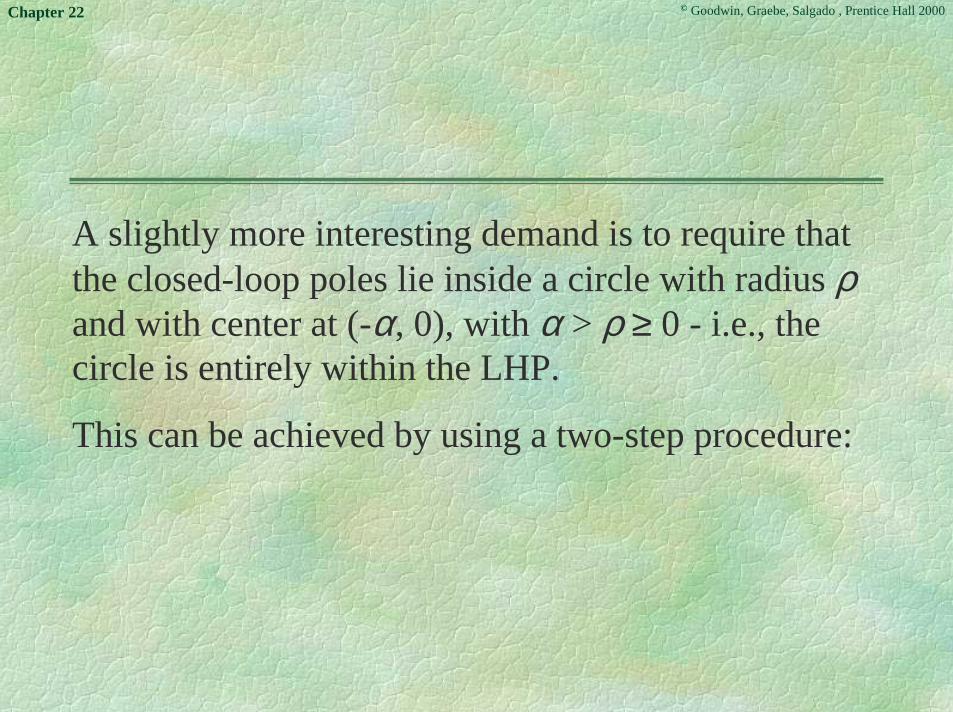
A slightly more interesting demand is to require thatthe closed-loop poles lie inside a circle with radius ρand with center at (-α, 0), with α > ρ ≥ 0 - i.e., thecircle is entirely within the LHP.
This can be achieved by using a two-step procedure:

© Goodwin, Graebe, Salgado , Prentice Hall 2000Chapter 22
(i) We first transform the Laplace variable s to a newvariable, ζ, defined as follows:
This takes the original circle is s to a unit circle in ζ .The corresponding transformed state space model has theform
ζ =s+ α
ρ
ζX(ζ) =1ρ(αI + Ao)X(ζ) +
1ρBoU(ζ)

© Goodwin, Graebe, Salgado , Prentice Hall 2000Chapter 22
(ii) One then treats the above model as the state spacedescription of a discrete-time system. So, solving thecorresponding discrete optimal control problem leads to afeedback gain K such that 1/ρ (αI + Ao - BoK) has all itseigenvalues inside the unit disk. This in turn implies that,when the same control law is applied in continuous time,then the closed-loop poles reside in the original circle ins .

© Goodwin, Graebe, Salgado , Prentice Hall 2000Chapter 22
Example
Consider a 2 × 2 multivariable system having thestate space model
Find a state-feedback gain matrix K such that theclosed-loop poles are all located in the disk withcenter at (-α; 0) and with radius ρ, where α = 6 andρ = 2.
Ao =
1 1 12 −1 03 −2 2
; Bo =
0 11 02 −1
; Co =
[1 0 00 1 0
]; Do = 0

© Goodwin, Graebe, Salgado , Prentice Hall 2000Chapter 22
We use the approach proposed above:
We first need the state space representation in thetransformed space.
A =1ρ(αI + Ao) and B =
1ρBo
© Goodwin, Graebe, Salgado , Prentice Hall 2000Chapter 22
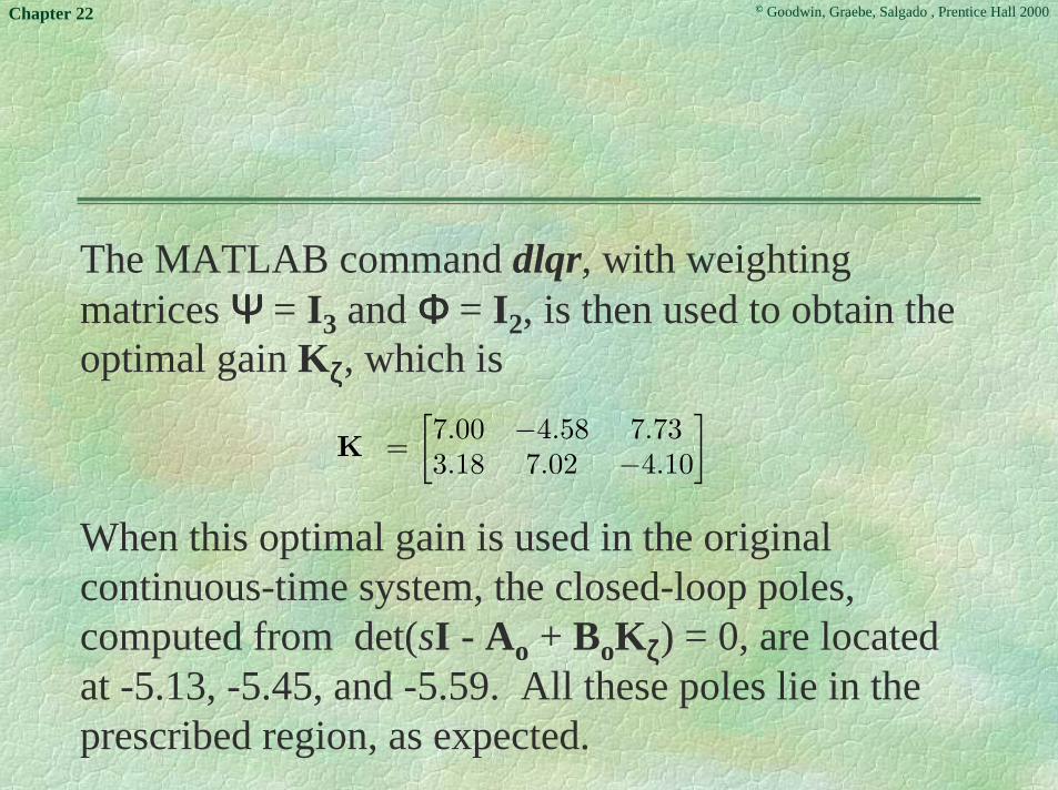
The MATLAB command dlqr, with weightingmatrices ΨΨΨΨ = I3 and ΦΦΦΦ = I2, is then used to obtain theoptimal gain Kζζζζ, which is
When this optimal gain is used in the originalcontinuous-time system, the closed-loop poles,computed from det(sI - Ao + BoKζζζζ) = 0, are locatedat -5.13, -5.45, and -5.59. All these poles lie in theprescribed region, as expected.
K =[7.00 −4.58 7.733.18 7.02 −4.10
]

© Goodwin, Graebe, Salgado , Prentice Hall 2000Chapter 22
Observer Design
Next, we turn to the problem of state estimation.Here, we seek a matrix J ∈ �n×p such that A - JC hasits eigenvalues inside the stability region. Again, it isconvenient to use quadratic optimization.

© Goodwin, Graebe, Salgado , Prentice Hall 2000Chapter 22
As a first step, we note that an observer can be designedfor the pair (C, A) by simply considering an equivalent(called dual) control problem for the pair (A, B). Toillustrate how this is done, consider the dual system with
Then, using any method for state-feedback design, wecan find a matrix K′ ∈ �p×n such that A′ - B′K′ has itseigenvalues inside the stability region. Hence, if wechoose J = (K′)T, then we have ensured that A - JC hasits eigenvalues inside the stability region. Thus, we havecompleted the observer design.
A′ = AT B′ = CT

© Goodwin, Graebe, Salgado , Prentice Hall 2000Chapter 22
The procedure leads to a stable state estimation of theform
Of course, using the tricks outlined above for state-variable feedback, one can also use transformationtechniques to ensure that the poles describing theevolution of the observer error also end up in anyregion that can be related to either the continuous- orthe discrete-time case by a rational transformation.
˙x(t) = Aox(t) + Bou(t) + J(y(t)− Cx(t))

© Goodwin, Graebe, Salgado , Prentice Hall 2000Chapter 22
We will show how the above procedure can beformalized by using Optimal Filtering theory. Theresulting optimal filter is called a Kalman filter.

© Goodwin, Graebe, Salgado , Prentice Hall 2000Chapter 22
Linear Optimal Filters
We will present one derivation of the optimal filtersbased on stochastic modeling of the noise. Analternative derivation based on model matching isgiven in the book.

© Goodwin, Graebe, Salgado , Prentice Hall 2000Chapter 22
Derivation Based on a StochasticNoise Model
We show how optimal-filter design can be set -up asa quadratic optimization problem. This shows thatthe filter is optimal under certain assumptionsregarding the signal-generating mechanism. Inpractice, this property is probably less important thanthe fact that the resultant filter has the right kind oftuning knobs so that it can be flexibly applied to alarge range of problems of practical interest.

© Goodwin, Graebe, Salgado , Prentice Hall 2000Chapter 22
Details of the Stochastic Model
Consider a linear stochastic system of the form
where dv(t) dw(t) are known as orthogonalincrement processes.
dx(t) = Ax(t)dt+ dw(t)dy(t) = Cx(t)dt+ dv(t)
© Goodwin, Graebe, Salgado , Prentice Hall 2000Chapter 22
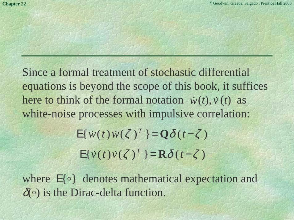
Since a formal treatment of stochastic differentialequations is beyond the scope of this book, it sufficeshere to think of the formal notation (t), (t) aswhite-noise processes with impulsive correlation:
where E{�} denotes mathematical expectation andδ(�) is the Dirac-delta function.
w� v�
)(})()({ ζδζ −= twtw T Q��E
)(})()({ ζδζ −= tvtv T R��E

© Goodwin, Graebe, Salgado , Prentice Hall 2000Chapter 22
We can then informally write the model as
For readers familiar with the notation of spectral densityfor random processes, we are simply requiring that thespectral density for (t) and (t) be Q and R,respectively.
w� v�
dx(t)dt
= Ax(t) +dw(t)dt
y′(t) =dy(t)dt
= Cx(t) +dv(t)dt

© Goodwin, Graebe, Salgado , Prentice Hall 2000Chapter 22
Our objective will be to find a linear filter driven byy′(t) that produces a state estimate having leastpossible error (in a mean square sense). We willoptimize the filter by minimizing the quadratic function
where
is the estimation error.
We will proceed to the solution of this problem in foursteps.
)(ˆ tx
Jt = E{x(t)x(t)T }
x(t) = x(t)− x(t)

© Goodwin, Graebe, Salgado , Prentice Hall 2000Chapter 22
Step 1:Consider a time-varying version of the model given by
where and have zero mean and areuncorrelated, and
dxz(t)dt
= Az(t)x(t) + wz(t)
y′z(t) =dyz(t)dt
= Cz(t)xz(t) + vz(t)
)( twz� )( tv z�
)()(})()({)()(})()({
ζδζζδζ
−=−=
ttvtvttwtw
Tzz
Tzz
z
z
RQ
��
��
E
E

© Goodwin, Graebe, Salgado , Prentice Hall 2000Chapter 22
For this model, we wish to compute
We assume that with (t)uncorrelated with the initial state xz(0) = xoz .
}.)()({)( Tzz txtxt E=P
,)0()0({ oP=Tzz xxE zw�
© Goodwin, Graebe, Salgado , Prentice Hall 2000Chapter 22
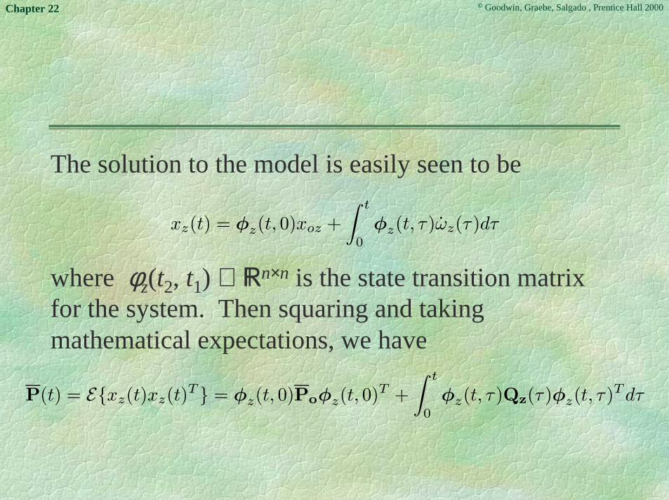
The solution to the model is easily seen to be
where φz(t2, t1) ∈ �n×n is the state transition matrixfor the system. Then squaring and takingmathematical expectations, we have
xz(t) = φz(t, 0)xoz +∫ t
0
φz(t, τ )ωz(τ )dτ
P(t) = E{xz(t)xz(t)T} = φz(t, 0)Poφz(t, 0)T +
∫ t
0
φz(t, τ )Qz(τ )φz(t, τ )Tdτ

© Goodwin, Graebe, Salgado , Prentice Hall 2000Chapter 22
Differentiating the above equation and using theLeibnitz rule, we obtain
where we have also used the fact that d/dt φ(t, τ) =Az(t)φ(t, τ).
dP(t)dt
= AzP(t) + P(t)AzT + Qz(t)

© Goodwin, Graebe, Salgado , Prentice Hall 2000Chapter 22
Step 2:We now return to the original problem: to obtain anestimate, for the state, x(t). We make asimplifying assumption by fixing the form of the filter.That is, we assume the following linear form for thefilter:
where J(t) is a time-varying gain yet to be determined.
),(ˆ tx
dx(t)dt
= Ax(t) + J(t)[y′(t)− Cx(t)]

© Goodwin, Graebe, Salgado , Prentice Hall 2000Chapter 22
Step 3:Assume that we are also given an initial stateestimate having the statistical property
and assume, for the moment, that we are given somegain J(τ) for 0 ≤ τ ≤ t. Derive an expression for
oxE{(x(0)− xo)(x(0)− xo)T } = Po,
P(t) = E{(x(t)− x(t))(x(t)− x(t))T}= E{x(t)x(t)T }

© Goodwin, Graebe, Salgado , Prentice Hall 2000Chapter 22
Solution: Subtracting the model from the filter format,we obtain
We see that this is a time-varying system, and we cantherefore immediately apply the solution to Step 1, aftermaking the following connections:
to conclude
subject to P(0) = Po. Note that we have used the fact thatQz(t) = J(t)RJ(t)T + Q.
dx(t)dt
= (A − J(t)C)x(t) + J(t)v(t)− w(t)
xz(t) → x(t); Az(t) → (A − J(t)C); wz(t) → J(t)v(t)− w(t)
dP(t)dt
= (A − J(t)C)P(t) + P(t)(A− J(t)C)T + J(t)RJ(t)T + Q

© Goodwin, Graebe, Salgado , Prentice Hall 2000Chapter 22
Step 4:We next choose J(t), at each time instant, so that isas small as possible.Solution: We complete the square on the right-handside of
by defining J(t) = J*(t) + J(t) where J*(t) = P(t)CTR-1.
P�
dP(t)dt
= (A − J(t)C)P(t) + P(t)(A− J(t)C)T + J(t)RJ(t)T + Q

© Goodwin, Graebe, Salgado , Prentice Hall 2000Chapter 22
Substituting into the equation for P(t) gives:
We clearly see that is minimized at every timeif we choose Thus, J*(t) is the optimal-filter gain, because it minimizes (and henceP(t)) for all t.
dP(t)dt
=(A − J(t)C− J(t)C)P(t) + P(t)(A− J(t)C− J(t)C)T
+ (J∗(t) + J(t))R(J∗(t) + J(t))T + Q
=(A − J(t)C)P(t) + P(t)(A− J(t)C)T
+ J∗(t)RJ∗(t) + Q + J(t)R(J(t))T
)( tP�0.)(~ =tJ
)( tP�

© Goodwin, Graebe, Salgado , Prentice Hall 2000Chapter 22
In summary, the optimal filter satisfies
where the optimal gain J*(t) satisfies
and P(t) is the solution to
subject to P(0) = Po.
dx(t)dt
= Ax(t) + J∗(t)[y′(t)− Cx(t)]
J∗(t) = P(t)CTR−1
dP(t)dt
=(A − J∗(t)C)P(t) + P(t)(A− J∗(t)C)T
+ J∗(t)R(J∗(t))T + Q

© Goodwin, Graebe, Salgado , Prentice Hall 2000Chapter 22
The key design equation for P(t) is
This can also be simplified to
The reader will recognize that the solution to the optimallinear filtering problem presented above has a very closeconnection to the LQR problem presented earlier. Thisis not surprising in view of the duality idea mentionedearlier
dP(t)dt
=(A − J∗(t)C)P(t) + P(t)(A− J∗(t)C)T
+ J∗(t)R(J∗(t))T + Q
dP(t)dt
= Q− P(t)CTR−1CP(t) + P(t)AT + AP(t)

© Goodwin, Graebe, Salgado , Prentice Hall 2000Chapter 22
Time Varying Systems ?
It is important to note, in the above derivation, that itmakes no difference whether the system is timevarying (i.e., A, C, Q, R, etc. are all functions oftime). This is often important in applications.

© Goodwin, Graebe, Salgado , Prentice Hall 2000Chapter 22
Properties ?
When we come to properties of the optimal filter,these are usually restricted to the time-invariant case(or closely related cases - e.g., periodic systems).Thus, when discussing the steady-state filter, it isusual to restrict attention to the case in which A, C,Q, R, etc. are not explicit functions of time.
The properties of the optimal filter then followdirectly from the optimal LQR solutions, under thecorrespondences given in Table 22.10 on the nextslide.

© Goodwin, Graebe, Salgado , Prentice Hall 2000Chapter 22
Regulator Filter
τ t− τ
tf 0
A −AT
B −CT
Ψ Q
Φ R
Ψf Po
Table 22.1: Duality between quadratic regulators and filters
Note that, using the above correspondences, one canconvert an optimal filtering problem into an optimalcontrol problem and vice versa.

© Goodwin, Graebe, Salgado , Prentice Hall 2000Chapter 22
In particular, one is frequently interested in thesteady-state optimal filter obtained when A, C, Q andR are time invariant and the filtering horizon tends toinfinity. By duality with the optimal controlproblem, the steady-state filter takes the form
where
and Ps∞ is the stabilizing solution of the following
CTARE:
dx(t)dt
= Ax+ J∞s (y′ − Cx)
J∞s = Ps
∞CT R−1
Q− P∞CT R−1CP∞ + P∞AT + AP∞ = 0

© Goodwin, Graebe, Salgado , Prentice Hall 2000Chapter 22
We state without proof the following facts that arethe duals of those given for the LQP.(i) Say that the system (C, A) is detectable from y(t); and
(ii) Say that the system states are all perturbed by noise. (Technically, this is stated as requiring that (A, Q½) is stabilizable).

© Goodwin, Graebe, Salgado , Prentice Hall 2000Chapter 22
Then, the optimal solution of the filtering Riccatiequation tends to a steady-state limit Ps
∞ as t → ∞.This limit has two key properties:
◆ Ps∞ is the only nonnegative solution of the matrix
algebraic Riccati Equation
obtained by setting dP(t)/dt inQ− P∞CT R−1CP∞ + P∞AT + AP∞ = 0
dP(t)dt
= Q− P(t)CTR−1CP(t) + P(t)AT + AP(t)

© Goodwin, Graebe, Salgado , Prentice Hall 2000Chapter 22
◆ When this steady-state value is used to generate asteady-state observer, then the observer has theproperty that (A - Js
∞C) is a stability matrix.
Note that this gives conditions under which a stablefilter can be designed. Placing the filter poles inparticular regions follows the same ideas as usedearlier in the case of optimal control.

© Goodwin, Graebe, Salgado , Prentice Hall 2000Chapter 22
Discrete-Time Optimal QuadraticFilterWe can readily develop discrete forms for the optimal filter.In particular, consider a discrete-time system having thefollowing state space description:
where w[k] ∈ �n and v[k] ∈ �n are uncorrelated stationarystochastic processes, with covariances given by
where Q ∈ �n×p is a symmetric nonnegative definite matrixand R ∈ �n×p is a symmetric positive definite matrix
x[k + 1] = Ax[k] + Bu[k] + w[k]y[k] = C[k] + v[k]
E{w[k]wT [ζ]} = QδK [k − ζ]
E{v[k]vT [ζ]} = RδK [k − ζ]

© Goodwin, Graebe, Salgado , Prentice Hall 2000Chapter 22
Consider now the following observer to estimate thesystem state:
Furthermore, assume that the initial state x[0] satisfies
Then the optimal choice (in a quadratic sense) for theobserver gain sequence {Jo[k]} is given by
where P[k] satisfies the following discrete-time dynamicRiccati equation (DTDRE).
x[k + 1] = Ax[k] + Bu[k] + Jo[k](y[k]− Cx[k]
)
E{(x[0]− x[0])(x[0]− x[0])T } = Po
Jo[k] = AP[k]CT(R + CP[k]CT
)−1

© Goodwin, Graebe, Salgado , Prentice Hall 2000Chapter 22
which can be solved forward in time, subject to
P[k + 1] = A(P[k]− P[k]CT
(R + CP[k]CT
)−1CP[k]
)AT + Q
P[0] = Po

© Goodwin, Graebe, Salgado , Prentice Hall 2000Chapter 22
The steady-state (k → ∞) filter gain satisfies theDTARE given by
A[P∞ − P∞CT
(R + CP∞CT
)−1CP∞
]AT + Q = P∞
© Goodwin, Graebe, Salgado , Prentice Hall 2000Chapter 22
Stochastic Noise Models
In the above development, we have simply representedthe noise as a white-noise sequence ({ω(k)}) and awhite measurement-noise sequence ({υ(k)}). Actually,this is much more general than it may seem at firstsight. For example, it can include colored noise havingan arbitrary rational noise spectrum. The essential ideais to model this noise as the output of a linear system(i.e., a filter) driven by white noise.

© Goodwin, Graebe, Salgado , Prentice Hall 2000Chapter 22
Thus, say that a system is described by
where {ωc(k)} represents colored noise - noise that iswhite noise passed through a filter. Then we can addthe additional noise model to the description. Forexample, let the noise filter be
where {ω(k)} is a white-noise sequence.
x(k + 1) = Ax(k) + Bu(k) + ωc(k)y(k) = Cx(k) + υ(k)
x′(k + 1) = A′x(k) + ω(k)ωc(k) = C′x′(k)

© Goodwin, Graebe, Salgado , Prentice Hall 2000Chapter 22
This yields a composite system driven by white noise,of the form
x(k + 1) = Ax(k) + Bu(k) + ω(k)y(k) = Cx(k) + υ(k)
where
x(k) = [x(k)T , x′(k)T ]T
ω(k) = [0, ω(k)T ]
A =[A C′
0 A′
]; B =
[B0
]; C =
[C 0
]

© Goodwin, Graebe, Salgado , Prentice Hall 2000Chapter 22
Because of the importance of the discrete KalmanFilter in applications, we will repeat below theformulation and derivation. The discrete derivationmay be easier to follow than the continuous casegiven earlier.

© Goodwin, Graebe, Salgado , Prentice Hall 2000Chapter 22
Discrete-Time State-Space Model
kk
kkk
xyBuxx
CA
=+=+1
The above state-space system is deterministic since nonoise is present.

© Goodwin, Graebe, Salgado , Prentice Hall 2000Chapter 22
We can introduce uncertainty into the model byadding noise terms
This is referred to as a stochastic state-space model.
kkkk wuxx ++=+ BA1
kkk nxy +=C
Processnoise
Measurementnoise

© Goodwin, Graebe, Salgado , Prentice Hall 2000Chapter 22
In particular, for a 3rd Order System we have:
kkkk wuxx ++=+ BA1
kkk nxy +=C
Processnoise
Measurementnoise
k
k
kkwww
uxxx
xxx
��
�
�
��
�
�+
��
�
�
��
�
�+
��
�
�
��
�
�
��
�
�
��
�
�=
��
�
�
��
�
�
+3
2
1
3
2
1
3
2
1
333231
232221
131211
13
2
1
BBB
AAAAAAAAA
( ) )()(3
2
1
321k
k
k nxxx
y +��
�
�
��
�
�= CCC

© Goodwin, Graebe, Salgado , Prentice Hall 2000Chapter 22
xk3 ˜ y k
B, A C + +
xk1
xk2
yk
nk
wk
uk
~
Xk - state vectorA - system matrixB - input matrixC - output matrixyk - output (PVm)yk - noise free output (PV)wk - process noisenk - measurement noiseuk - control input (MV)
This is illustrated below:

© Goodwin, Graebe, Salgado , Prentice Hall 2000Chapter 22
We recall that a Kalman Filter is a particular type ofobserver. We propose a form for this observer on thenext slide.

© Goodwin, Graebe, Salgado , Prentice Hall 2000Chapter 22
ObserversWe are interested in constructing an optimal observerfor the following state-space model:
An observer is constructed as follows:
where J is the observer gain vector, and is thebest estimate of yk i.e.
kkk
kkkk
nxywuxx
+=++=+
CBA1
)ˆ(ˆˆ 1 kkkkk yyJuxx −++=+ BAky
.ˆˆ kk xy C=
© Goodwin, Graebe, Salgado , Prentice Hall 2000Chapter 22
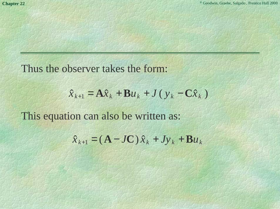
Thus the observer takes the form:
This equation can also be written as:
)ˆ(ˆˆ 1 kkkkk xyJuxx CBA −++=+
kkkk uJyxJx BCA ++−=+ ˆ)(ˆ 1
© Goodwin, Graebe, Salgado , Prentice Hall 2000Chapter 22
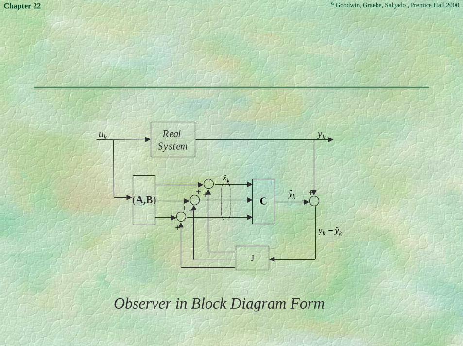
yk − ˆ y k
Real System
ykuk
ˆ y k
J
++++
++ _ +(A,B) C
ˆ x k�
�
� � � �
�
�
� � � �
Observer in Block Diagram Form
© Goodwin, Graebe, Salgado , Prentice Hall 2000Chapter 22
Kalman Filter
The Kalman filter is a special observer that hasoptimal properties under certain hypotheses. Inparticular, suppose that.
1) wk and nk are statistically independent (uncorrelated in time and with each other)
2) wk and nk, have Gaussian distributions3) The system is known exactly
The Kalman filter algorithm provides an observervector J that results in an optimal state estimate.

© Goodwin, Graebe, Salgado , Prentice Hall 2000Chapter 22
The optimal J is referred to as the Kalman Gain (J*)
k
kkkkk
xyyyJuxx
ˆˆ)ˆ(*ˆˆ 1
CBA
=−++=+
© Goodwin, Graebe, Salgado , Prentice Hall 2000Chapter 22
Five step Kalman Filter Derivation
Background:E[•] - Expected Value or Average
( ) [ ]( ) [ ]( ) matrixscalar
vector
−Σ==
−==Σ
222
2
var:
cov
wkkw
kTkkkw
wEw
wwwEw
σ
( ) [ ]( ) [ ]( ) matrixscalar
vector
−Σ==
−==Σ
222
2
var:
cov
nkkn
kTkkkn
nEn
nnnEn
σ
© Goodwin, Graebe, Salgado , Prentice Hall 2000Chapter 22
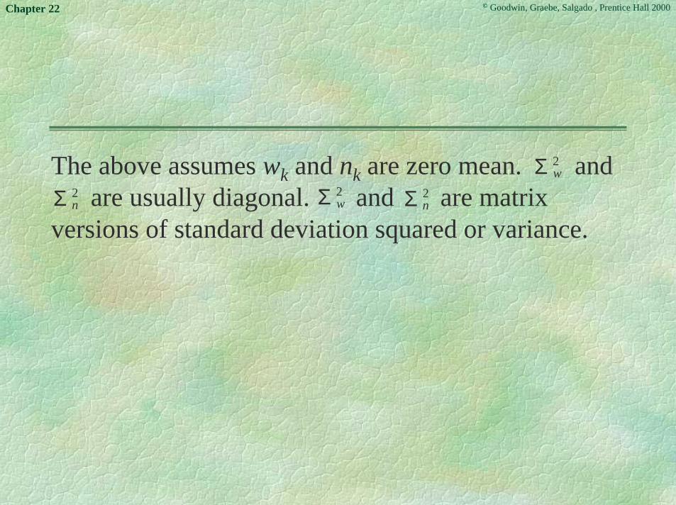
The above assumes wk and nk are zero mean. and are usually diagonal. and are matrixversions of standard deviation squared or variance.
2wΣ
2nΣ 2
wΣ 2nΣ

© Goodwin, Graebe, Salgado , Prentice Hall 2000Chapter 22
Step 1:Given
Calculate
�==+=+
2
000
1
][][
wTkk
T
kkk
wwEPxxEwxx A
][ Tkkk xxEP =

© Goodwin, Graebe, Salgado , Prentice Hall 2000Chapter 22
Solution:
[ ] ( )( )[ ]( )( )[ ]( ) ( ) ( ) ( )[ ][ ] [ ] ( ) [ ]
�+++=
+++=
+++=
++=
++=++
2
11
00 wT
k
Tkk
TTkk
Tkk
TTkk
Tkk
TTkk
Tkk
TTkk
Tk
TTkkk
Tkkkk
Tkk
wwExwEwxExxE
wwxwwxxxE
wxwxE
wxwxExxE
AAP
AAAA
AAAA
AA
AA
�+=+2
1 wT
kk AAPP

© Goodwin, Graebe, Salgado , Prentice Hall 2000Chapter 22
Step 2:
What is a good estimate of xk ?
We try the following form for the filter (where thesequence {Jk} is yet to be determined):
)ˆ(ˆˆˆ 1 kkkkkk xyJuxx CBA −++=+
kkk
kkkk
nxywuxx
+=++=+
CBA1

© Goodwin, Graebe, Salgado , Prentice Hall 2000Chapter 22
Step 3:Given
and
Evaluate:)ˆ(ˆˆ 1 kkkkkk xyJuxx CBA −++=+
kkk
kkkk
nxywuxx
+=++=+
CBA1
( )( )[ ]Tkkkkkk xxxxExx ˆˆ)ˆcov( −−=−
© Goodwin, Graebe, Salgado , Prentice Hall 2000Chapter 22
Solution:
( )( )
( ) kkkkk
kkkkkk
kkkkkkk
kkkkkkkkk
kkk
nJwxJnJwxJx
xJnxJwxxJyJuxwux
xxx
−+−=−+−=
++−+=−++−++=
−= +++
~~~
ˆ~ˆ
ˆ~111
CACA
CCACBABA

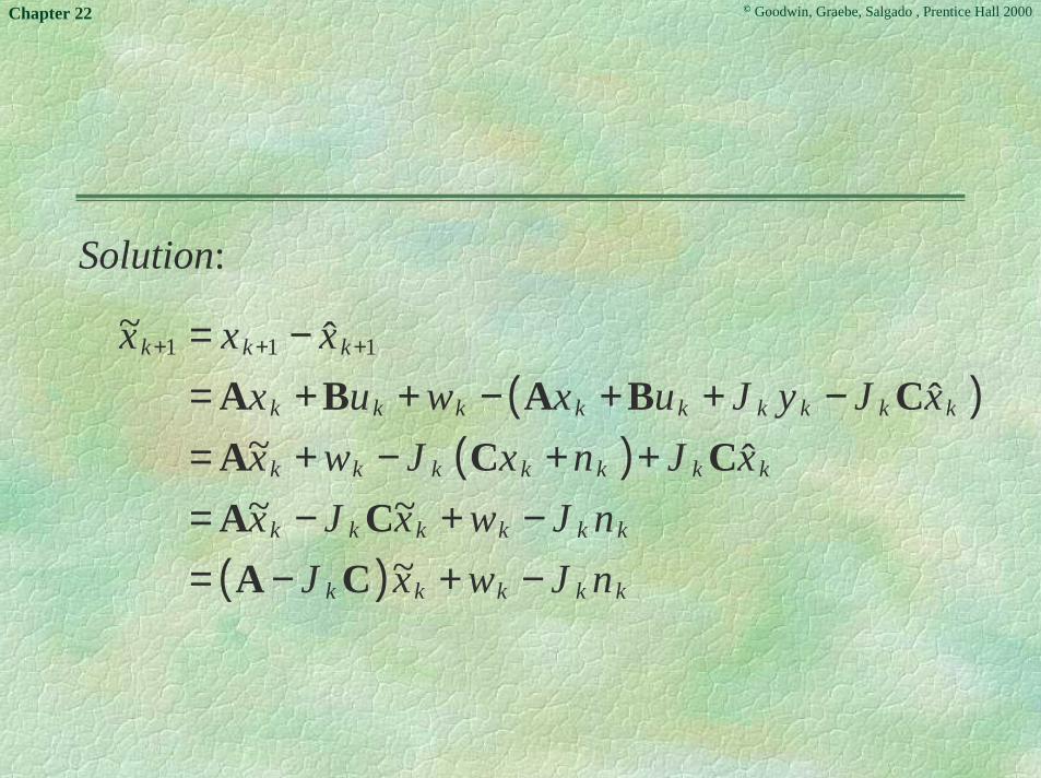
© Goodwin, Graebe, Salgado , Prentice Hall 2000Chapter 22
Let
Then applying the result of step 2 we have
[ ]Tkkk xxE 111
~~+++ =P
( ) ( ) �� ++−−=+22
1 nTkkw
Tkkkk JJJPJ CACAP

© Goodwin, Graebe, Salgado , Prentice Hall 2000Chapter 22
Step 4:Given
Evolves according to
What is the best (optimal) value for J (call it )?
[ ]Tkk xxE ~~=kP
( ) ( ) �� ++−−=+22
1 nTkkw
Tkkkk JJJJ CAPCAP
*kJ

© Goodwin, Graebe, Salgado , Prentice Hall 2000Chapter 22
Solution:
Since Pk+1 is quadratic in Jk, it seems we should beable to determine Jk so as to minimize Pk+1.We first consider the scalar case.
© Goodwin, Graebe, Salgado , Prentice Hall 2000Chapter 22
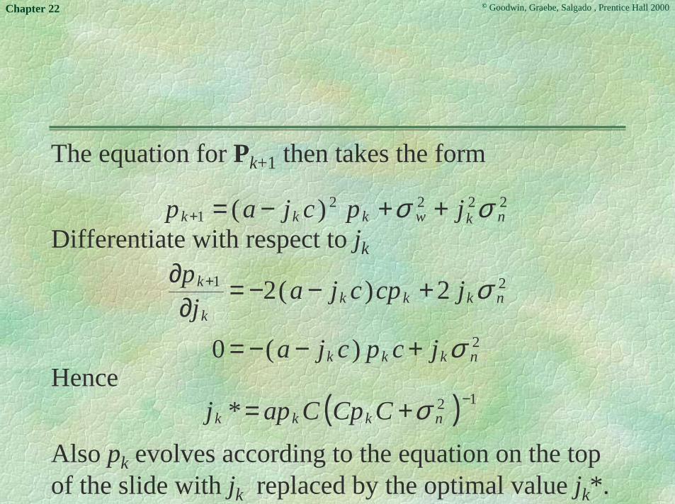
The equation for Pk+1 then takes the form
Differentiate with respect to jk
Hence
Also pk evolves according to the equation on the topof the slide with jk replaced by the optimal value jk*.
22221 )( nkwkkk jpcjap σσ ++−=+
2
21
)(0
2)(2
nkkk
nkkkk
k
jcpcja
jcpcjaj
p
σ
σ
+−−=
+−−=∂
∂ +
( ) 12* −+= nkkk CCpCapj σ
© Goodwin, Graebe, Salgado , Prentice Hall 2000Chapter 22
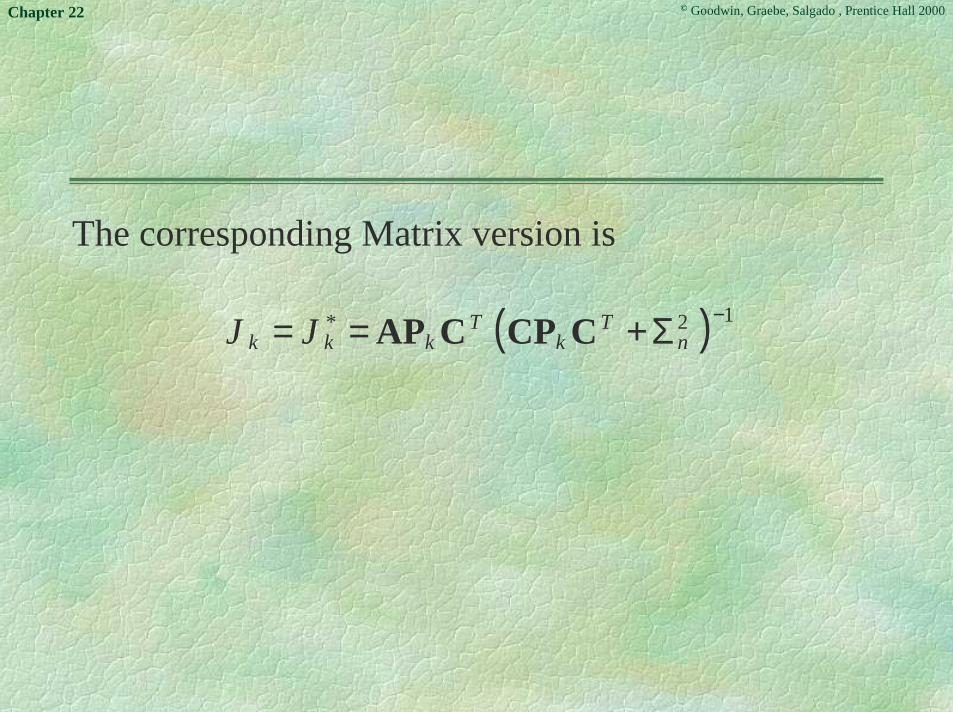
The corresponding Matrix version is
( ) 12* −Σ+== nT
kT
kkk JJ CCPCAP

© Goodwin, Graebe, Salgado , Prentice Hall 2000Chapter 22
Step 5:Bring it all together.Given
where
Find optimal filter.
kkk
kkkk
nxywuxx
+=++=+
CBA1
[ ][ ]( )( )[ ]
=−−=
=Σ=Σ
0
00000
2
2
ˆˆˆ
xxxxxEP
nnEwwE
T
Tkkw
Tkkw
Initial state estimate

© Goodwin, Graebe, Salgado , Prentice Hall 2000Chapter 22
Solution:The Kalman Filter
)ˆ(ˆˆˆ *1 kkkkkk xyJuxx CBA −++=+
( ) 12* −Σ+= nTT
kkJ CPCCAP
( ) ( )( )( ) 212
2*2**1 *
wT
knT
kT
kk
nT
kwT
kkkk JJJJ
�+�+−=
++−−=−
+ ��
ACPCCPCPPA
CAPCAP

© Goodwin, Graebe, Salgado , Prentice Hall 2000Chapter 22
Simple ExampleProblem:Estimate a constant from measurements yk corrupted bywhite noise of variance 1.
Model for constant � xk+1 = xk; wk = 0
Model for the corrupted measurement � yk = xk + nk
An initial estimate of this constant is given, but thisinitial estimate has a variance of 1 around the true value.
[ ] ( ) 1var 22 =�==� nkk nnE

© Goodwin, Graebe, Salgado , Prentice Hall 2000Chapter 22
Solution Formulation( )[ ] ( )
1;0;0;1
1ˆvarˆ22
0002
00
=�=�==
==−=−
nw
xxxxE
BA
P
From previous Kalman Filter equations with A = 1; B = 0;C = 1; �w
2 = 0; �n2 = 1
1
1
)ˆ(ˆˆ
2
1
*
*1
+−=
+=
−+=
+
+
k
kkk
k
kk
kkkkk
J
xyJxx
PPPP
PP

© Goodwin, Graebe, Salgado , Prentice Hall 2000Chapter 22
Calculate Pk (Given P0 = 1)
( )
;61,
51,
41
31
121
1
21
1111
1
543
21
221
1
21
12
2
0
20
01
===
=+
−=+
−=
=+
−=+
−=
PPP
PPPP
PPPP
etc.

© Goodwin, Graebe, Salgado , Prentice Hall 2000Chapter 22
Calculate the estimate given the initial estimateand the noisy measurements yk
kx 0x
( )
( )
( )00
000
000
001
ˆ21
ˆ111ˆ
ˆ1ˆˆ
yx
xyx
xyxx
+=
−+
+=
−+
+=P
P

© Goodwin, Graebe, Salgado , Prentice Hall 2000Chapter 22
( )
( ) ( )( )( )
( )
( )321004
21003
100
00121
21
00
111
112
ˆ51ˆ
ˆ41ˆ
ˆ31
ˆ21
1ˆ2
1
ˆ1ˆˆ
yyyyxx
yyyxx
yyx
yxyyx
xyxx
++++=
+++=
++=
+−+
++=
−+
+=P
P

© Goodwin, Graebe, Salgado , Prentice Hall 2000Chapter 22
The above result (for this special problem) is intuitivelyreasonable. Note that the Kalman Filter has simplyaveraged the measurements and has treated the initialestimate as an extra piece of information (like an extrameasurement). This is probably the answer you wouldhave guessed for estimating the constant before youever heard of the Kalman Filter.
The fact that the answer is heuristically reasonable inthis special case encourages us to believe that theKalman Filter may give a good solution in other, morecomplex cases. Indeed it does !

© Goodwin, Graebe, Salgado , Prentice Hall 2000Chapter 22
State-Estimate FeedbackFinally, we can combine the state estimation providedby the Kalman Filter with the state-variable feedbackdetermined earlier to yield the following state-estimatefeedback-control law:
Note that the closed-loop poles resulting from the use ofthis law are the union of the eigenvalues that result fromthe use of the state feedback together with theeigenvalues associated with the observer. Actually, theresult can also be shown to be optimal via StochasticDynamic Programming. (However, this is beyond thescope of the treatment presented here).
u(t) = −Kx(t) + r(t)

© Goodwin, Graebe, Salgado , Prentice Hall 2000Chapter 22
Achieving Integral Action in LQRSynthesis
An important aspect not addressed so far is thatoptimal control and optimal state-estimate feedbackdo not automatically introduce integral action. Thelatter property is an architectural issue that has to beforced onto the solution.
One way of forcing integral action is to put a set ofintegrators at the output of the plant.

© Goodwin, Graebe, Salgado , Prentice Hall 2000Chapter 22
This can be described in state space form as
As before, we can use an observer (or Kalman filter) toestimate x from u and y. Hence, in the sequel we willassume (without further comment) that x and z are directlymeasured. The composite system can be written in statespace form as
x(t) = Ax(t) + Bu(t)y(t) = Cx(t)z(t) = −y(t)
x′(t) = A
′x(t) + B
′u(t)

© Goodwin, Graebe, Salgado , Prentice Hall 2000Chapter 22
Where
We then determine state feedback (from x′(t)) tostabilize the composite system.
x′=[x(t)z(t)
]; A
′=[
A 0−C 0
]; B′ =
[B0
]

© Goodwin, Graebe, Salgado , Prentice Hall 2000Chapter 22
The final architecture of the control system wouldthen appear as below.
Figure 22.2: Integral action in MIMO control
y∗(t)
u(t) z(t)
x(t)Observer
Plant
parallelintegrators
Feedbackgain
+
−
y(t) e(t)z(t) = e(t)

© Goodwin, Graebe, Salgado , Prentice Hall 2000Chapter 22
Industrial Applications
Multivariable design based on LQR theory and theKalman filter accounts for thousands of real-worldapplications.
The key issue in using these techniques in practicelies in the problem formulation; once the problemhas been properly posed, the solution is usually ratherstraightforward. Much of the success in applicationsof this theory depends on the formulation, so we willconclude this chapter with brief descriptions of fourreal-world applications.

© Goodwin, Graebe, Salgado , Prentice Hall 2000Chapter 22
Geostationary Satellite Tracking
It is known that so-called geostationary satellitesactually appear to wobble in the sky. The period ofthis wobble is one sidereal day. If one wishes topoint a receiving antenna exactly at a satellite so as tomaximize the received signal, then it is necessary totrack this perceived motion. The required pointingaccuracy is typically to within a few hundredths of adegree. The physical set-up is as shown in the nextfigure.

© Goodwin, Graebe, Salgado , Prentice Hall 2000Chapter 22
Figure 22.4: Satellite and antenna angle definitions

© Goodwin, Graebe, Salgado , Prentice Hall 2000Chapter 22
One could use an open-loop solution to this problem, asfollows: Given a model (e.g., a list of pointing anglesversus time), the antenna could be pointed in the correctorientation as indicated by position encoders. Thistechnique is used in practice, but it suffers from thefollowing practical issues:
◆ It requires high absolute accuracy in the position encoders,antenna, and reflector structure.
◆ It also requires regular maintenance to put in new modelparameters
◆ It cannot compensate for wind, thermal, and other time-varying effects on the antenna and reflector.

© Goodwin, Graebe, Salgado , Prentice Hall 2000Chapter 22
This motivates the use of a closed-loop solution. Insuch a solution, the idea is to move the antennaperiodically so as to find the direction of maximumsignal strength. However, the data so received are noisyfor several reasons, including the following:
◆ noise in the received signal, p;◆ variations in the signal intensity transmitted from the
satellite;◆ imprecise knowledge of the beam pattern for the antenna;
and◆ the effect of wind gusts on the structure and the reflector.

© Goodwin, Graebe, Salgado , Prentice Hall 2000Chapter 22
It is a reasonable hypothesis that we can smooth thisdata by using a Kalman filter. Toward this end, weneed first to build a model for the orbit. Now, as seenfrom the earth, the satellite executes a periodic motionin the two axes of the antenna (azimuth and elevation -see next slide). Several harmonics are present but thedominant harmonic is the fundamental. This leads to amodel of the formwhere ΨΨΨΨs(t) is, say, the azimuth angle as a function oftime. The frequency ω in this application is known.There are several ways of describing this model in statespace form.
y(t) = Ψs(t) = x1 + x2 sinωt+ x3 cosωt

© Goodwin, Graebe, Salgado , Prentice Hall 2000Chapter 22
ψ s ( t )
Time
Typical inclined orbit satellite motion
Typical satellite motion is close to periodic, with aperiod of 1 sidereal day:

© Goodwin, Graebe, Salgado , Prentice Hall 2000Chapter 22
xtCtxtxxts
)()cos()sin()( 321
=++≈ ωωψ
[ ][ ]321
)cos()sin(1)(
xxxx
tttCT =
= ωω
Linear Model:
with
Several Harmonics are present, but the dominant harmonic is the fundamental:

© Goodwin, Graebe, Salgado , Prentice Hall 2000Chapter 22
This can be expressed in state space form as follows:
d
dt
x1
x2
x3
= 0
y(t) = C(t)x(t)
where C(t) = [1, sinωt, cosωt]

© Goodwin, Graebe, Salgado , Prentice Hall 2000Chapter 22
Given noisy measurements, y(t), fit a model for the unknown parameters x1, x2 and x3.
This system is time-varying (actually periodic). We can then immediately apply the Kalman filter to estimate x1, x2 and x3 from noisy measurements of y(t).
Problem Reformulation:
© Goodwin, Graebe, Salgado , Prentice Hall 2000Chapter 22
In practice, it is important to hypothesise theexistence of a small amount of fictitious processnoise which is added to the model equations. Thisrepresents the practical fact that the model isimprecise. This leads to a filter which is robust to themodel imprecision.

© Goodwin, Graebe, Salgado , Prentice Hall 2000Chapter 22
One can formally derive properties of the resultingfilter. Heuristically one would expect:
◆ As one increases the amount of hypothesised model error,the filter pays more attention to the measurements, i.e. thefilter gain increases;
◆ As one decreases the amount of hypothesised model error,the filter pays more attention to the model. In particular,the filter will ultimately ignore the measurements after aninitial transient if one assumes no model error.
The above heuristic ideas can, in fact, be formallyestablished.
© Goodwin, Graebe, Salgado , Prentice Hall 2000Chapter 22
To initialize the filter one needs;◆ a guess at the current satellite orientation;
◆ a guess at the covariance of the initial state error (P(0));
◆ a guess at the measurement-noise intensity (R); and
◆ a rough value for the added process noise intensity (Q).

© Goodwin, Graebe, Salgado , Prentice Hall 2000Chapter 22
A commercial system built around the aboveprinciples has been designed and built at theUniversity of Newcastle, Australia. This system ismarketed under the trade name ORBTRACK andhas been used in many real-world applicationsranging from Australia to Indonesia and Antarctica.See next slide for photo.

© Goodwin, Graebe, Salgado , Prentice Hall 2000Chapter 22
ORBTRACK

© Goodwin, Graebe, Salgado , Prentice Hall 2000Chapter 22
Zinc Coating-Mass Estimation inContinuous Galvanizing Lines
A diagram of a continuous galvanizing line is shownon the next slide. An interesting feature of thisapplication is that the sheet being galvanized is ameter or so wide and many hundreds of meters long.
The strip passes through a zinc pot (as in the figure).Subsequently, excess zinc is removed by air knives.The strip then moves through a cooling section, andfinally the coating mass is measured by a traversingX-ray gauge.

© Goodwin, Graebe, Salgado , Prentice Hall 2000Chapter 22
Figure 22.5: Schematic diagram of continuous galvanizing line

© Goodwin, Graebe, Salgado , Prentice Hall 2000Chapter 22
The x ray gauge moves backwards and forwardsacross the moving strip as shown diagramatically onthe next slide.

© Goodwin, Graebe, Salgado , Prentice Hall 2000Chapter 22
Figure 22.6: Traversing X-ray gauge

© Goodwin, Graebe, Salgado , Prentice Hall 2000Chapter 22
If one combines the lateral motion of the X-ray gaugewith the longitudinal motion of the strip, then oneobtains the ziz-zag measurement pattern shownbelow.
Figure 22.7: Zig-zag measurement pattern

© Goodwin, Graebe, Salgado , Prentice Hall 2000Chapter 22
Because of the sparse measurement pattern, it is highlydesirable to smooth and interpolate the coating-massmeasurements. The Kalman filter is a possible tool tocarry out this data-smoothing function. However,before we can apply this tool, we need a model for therelevant components in the coating-mass distribution.The relevant components include the following:

© Goodwin, Graebe, Salgado , Prentice Hall 2000Chapter 22
◆ Shape Disturbances (arising from shape errors in therolling process).
These can be described by band-pass-filtered noise components, by using a model of the form
x1 =− ω1x1 −[
ω2ω1
ω2 − ω1
]n
x2 = −ω2x2 −[
ω22
ω1 − ω2
]n
ysd = (1, 1)(x1
x2
)
© Goodwin, Graebe, Salgado , Prentice Hall 2000Chapter 22
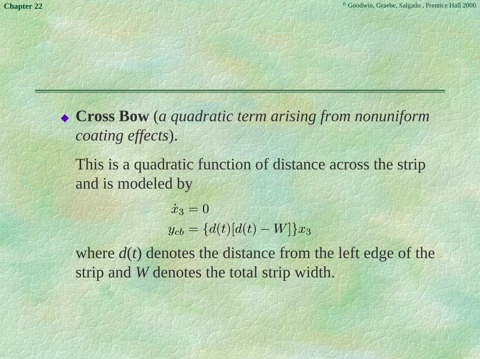
◆ Cross Bow (a quadratic term arising from nonuniformcoating effects).
This is a quadratic function of distance across the stripand is modeled by
where d(t) denotes the distance from the left edge of thestrip and W denotes the total strip width.
x3 = 0ycb = {d(t)[d(t)−W ]}x3

© Goodwin, Graebe, Salgado , Prentice Hall 2000Chapter 22
◆ Skew (due to misalignment of the knife jet)
This is a term that increases linearly with distance fromthe edge. It can thus be modeled by
x4 = 0ysc = {d(t)}x4

© Goodwin, Graebe, Salgado , Prentice Hall 2000Chapter 22
◆ Eccentricity (due to out-of-round in the rolls)
Say that the strip velocity is υs and that the roll radius isr. Then this component can be modeled as
x5 = 0x6 = 0
ye = {sin(υs
r
)t, cos
(υs
r
)t}(x5
x6
)

© Goodwin, Graebe, Salgado , Prentice Hall 2000Chapter 22
◆ Strip Flap (due to lateral movement of the strip in thevertical section of the galvanizing line)
Let f(t) denote the model for the flap; then thiscomponent is modeled by
x7 = 0
yf = {f(t)}x7

© Goodwin, Graebe, Salgado , Prentice Hall 2000Chapter 22
◆ Mean Coating Mass (the mean value of the zinc layer)
This can be simply modeled by
x8 = 0ym = x8

© Goodwin, Graebe, Salgado , Prentice Hall 2000Chapter 22
Putting all of the equations together gives us an 8th-ordermodel of the form
x = Ax+ Bn
z = y = C(t)x+ υ
A =
−ω1 0 0 0 0 0 0 00 −ω2 0 0 0 0 0 00 0 0 0 0 0 0 00 0 0 0 0 0 0 00 0 0 0 0 0 0 00 0 0 0 0 0 0 00 0 0 0 0 0 0 00 0 0 0 0 0 0 0
; B =
−(
ω2ω1ω2−ω1
)−(
ω22
ω1−ω2
)000000

© Goodwin, Graebe, Salgado , Prentice Hall 2000Chapter 22
Given the above model, one can apply the Kalmanfilter to estimate the coating-thickness model. Theresultant model can then be used to interpolate thethickness measurement. Note that here the Kalmanfilter is actually periodic, reflecting the periodicnature of the X-ray traversing system.
C = [1, 1, d(t)[d(t)−W ], d(t), sin(υs
dt), cos
(υs
dt), f(t), 1]

© Goodwin, Graebe, Salgado , Prentice Hall 2000Chapter 22
A practical form of this algorithm is part of acommercial system for Coating-Mass Controldeveloped in collaboration with the authors of thisbook by a company (Industrial Automation ServicesPty. Ltd.). The following slides are taken fromcommercial literature describing this Coating MassControl system.

© Goodwin, Graebe, Salgado , Prentice Hall 2000Chapter 22

© Goodwin, Graebe, Salgado , Prentice Hall 2000Chapter 22

© Goodwin, Graebe, Salgado , Prentice Hall 2000Chapter 22

© Goodwin, Graebe, Salgado , Prentice Hall 2000Chapter 22

© Goodwin, Graebe, Salgado , Prentice Hall 2000Chapter 22

© Goodwin, Graebe, Salgado , Prentice Hall 2000Chapter 22

© Goodwin, Graebe, Salgado , Prentice Hall 2000Chapter 22
Roll-Eccentricity Compensation inRolling Mills
The reader will recall that rolling-mill thickness-control problems were described in Chapter 8. Aschematic of the set-up is shown below.

© Goodwin, Graebe, Salgado , Prentice Hall 2000Chapter 22
Figure 22.8: Rolling-mill thickness control

© Goodwin, Graebe, Salgado , Prentice Hall 2000Chapter 22
F(t) : Forceh(t) : Exit-thickness Measurementu(t) : Unloaded Roll Gap (the control variable)
In Chapter 8, it was argued that the following virtualsensor (called a BISRA gauge) could be used toestimate the exit thickness and thus eliminate thetransport delay from mill to measurement.
h(t) =F (t)M
+ u(t)

© Goodwin, Graebe, Salgado , Prentice Hall 2000Chapter 22
However, one difficulty that we have not previouslymentioned with this virtual sensor is that the presenceof eccentricity in the rolls significantly affects theresults.
Figure 22.9: Roll eccentricity

© Goodwin, Graebe, Salgado , Prentice Hall 2000Chapter 22
To illustrate why this is so, let e denote the rolleccentricity. Then the true roll force is given by
In this case, the previous estimate of the thicknessobtained from the force actually gives
Thus, e(t) represents an error, or disturbance term, inthe virtual sensor output, one due to the effects ofeccentricity.
F (t) = M(h(t)− u(t) + e(t))
h(t) = h(t) + e(t)

© Goodwin, Graebe, Salgado , Prentice Hall 2000Chapter 22
This eccentricity component significantly degradesthe performance of thickness control using theBISRA gauge. Thus, there is strong motivation toattempt to remove the eccentricity effect from theestimated thickness provided by the BISRA gauge.

© Goodwin, Graebe, Salgado , Prentice Hall 2000Chapter 22
The next slide shows a simulation whichdemonstrates the effect of eccentricity on theperformance of a thickness control system in a rollingmill when eccentricity components are present.
◆ The upper trace shows the eccentricity signal◆ The second top trace shows another disturbance◆ The third top trace shows the effect of eccentricity in
the absence of feedback control◆ The bottom trace shows that when the eccentricity
corrupted BISRA gauge estimate is used in a feedbackcontrol system, then the eccentricity effect is magnified.

© Goodwin, Graebe, Salgado , Prentice Hall 2000Chapter 22

© Goodwin, Graebe, Salgado , Prentice Hall 2000Chapter 22
A key property that allows us to make progress onthe problem is that e(t) is actually (almost) periodic,because it arises from eccentricity in the four rolls ofthe mill (two work rolls and two back-up rolls).Also, the roll angular velocities are easily measuredin this application by using position encoders. Fromthis data, one can determine a multi-harmonic modelfor the eccentricity, of the form
e(t) =N∑
k=1
αk sinωkt+ βk cosωkt

© Goodwin, Graebe, Salgado , Prentice Hall 2000Chapter 22
Each sinusoidal input can be modeled by a secondorder state space model of the form
Finally, consider any given measurement, say theforce F(t). We can think of F(t) as comparing theabove eccentricity components buried in noise:
xk1(t) = ωkx
k2(t)
xk2(t) = −ωkx
k1(t)
y(t) = F (t) =N∑
k=1
xk1(t) + xk
2(t) + n(t)

© Goodwin, Graebe, Salgado , Prentice Hall 2000Chapter 22
We can then apply the Kalman filter to estimate
and hence to correct the measured force measurementsfor eccentricity.
Note that this application has much in common with thesatellite tracking problem since periodic functions areinvolved in both applications.
The final control system using the eccentricitycompensated BISRA gauge is as shown on the nextslide.
}...,,1);(),({ 21 Nktxtx kk =

© Goodwin, Graebe, Salgado , Prentice Hall 2000Chapter 22
Figure 22.10: Final roll eccentricity compensated control system

© Goodwin, Graebe, Salgado , Prentice Hall 2000Chapter 22
An interesting feature of this problem is that there issome practical benefit in using the general time-varyingform of the Kalman filter rather than the steady-statefilter. The reason is that, in steady state, the filter acts asa narrow band-pass filter bank centred on the harmonicfrequencies. This is, heuristically, the correct steady-statesolution. However, an interesting fact that the reader canreadily verify is that the transient response time of anarrow band-pass filter is inversely proportional to thefilter bandwidth. This means that, in steady state, one hasthe following fundamental design trade-off:

© Goodwin, Graebe, Salgado , Prentice Hall 2000Chapter 22
◆ On the one hand, one would like to have a narrow band-pass,to obtain good frequency selectivity and hence good noiserejection.
◆ On the other hand, one would like to have a wide band-pass,to minimize the initial transient period.
This is an inescapable dichotomy for any time-invariantfilter.This suggests that one should not use a fixed filter gainbut instead start with a wide-band filter, to minimize thetransient, but then narrow the filter band down as thesignal is acquired. This is precisely what the time-varying Kalman filter does.

© Goodwin, Graebe, Salgado , Prentice Hall 2000Chapter 22
The next slide shows the efficacy of using theKalman Filter to extract multiple sinusoidalcomponents from a composite signal.
◆ The upper trace shows the composite signal which maylook like random noise, but is in fact a combination ofmany sinewaves together with a noise component.
◆ The lower four traces show the extracted sinewavescorresponding to four of the frequencies. Note that afteran initial transient the filter output settles to thesinewave component in the composite signal.

© Goodwin, Graebe, Salgado , Prentice Hall 2000Chapter 22

© Goodwin, Graebe, Salgado , Prentice Hall 2000Chapter 22
The next slide shows a simulation which demonstratesthe advantages of using the Kalman Filter to compensatethe BISRA gauge by removing the eccentricitycomponents.
◆ The upper trace shows the uncontrolled response◆ The middle trace shows the exit thickness response when a
BISRA gauge is used but no eccentricity compensation isapplied
◆ The lower trace shows the controlled exit thickness whenthe BISRA gauge is used for feedback having first beencompensated using the Kalman Filter to remove theeccentricity components.

© Goodwin, Graebe, Salgado , Prentice Hall 2000Chapter 22

© Goodwin, Graebe, Salgado , Prentice Hall 2000Chapter 22
The next slide shows practical results of usingeccentricity compensation on a practical rolling mill.The results were obtained on a tandem cold milloperated by BHP Steel International.
◆ The upper trace is divided into two halves. The leftportion clearly shows the effect of eccentricity on therolled thickness whilst the right hand portion shows thedramatic improvement resulting from using eccentricitycompensation. Note that the drift in the mean on theright hand side is due to a different cause and can bereadily rectified.
© Goodwin, Graebe, Salgado , Prentice Hall 2000Chapter 22
◆ The remainder of the traces show the effect of using aneccentricity compensated BISRA gauge on a full coil.The traces also show lines at ±1% error which was thedesign goal at the time these results were collected.Note that it is now common to have accuracies of±0.1%

© Goodwin, Graebe, Salgado , Prentice Hall 2000Chapter 22

© Goodwin, Graebe, Salgado , Prentice Hall 2000Chapter 22
The final system, as described above, has beenpatented under the name AUSREC and is availableas a commercial product from Industrial AutomationServices Pty. Ltd.

© Goodwin, Graebe, Salgado , Prentice Hall 2000Chapter 22
Vibration Control in FlexibleStructures
Consider the problem of controller design for thepiezoelectric laminate beam shown on the next slide.

© Goodwin, Graebe, Salgado , Prentice Hall 2000Chapter 22
Figure 22.11: Vibration control by using a piezoelectric actuator
u(t) ytip(t)K(s)
y
r
This is a simple system. However, it represents manyof the features of more complex systems where onewishes to control vibrations. Such problems occur inmany problems, e.g. chatter in rolling mills, aircraftwing flutter, light weight space structures, etc.

© Goodwin, Graebe, Salgado , Prentice Hall 2000Chapter 22
In the laboratory system, the measurements are takenby a displacement sensor that is attached to the tip ofthe beam, and a piezoelectric patch is used as theactuator. The purpose of the controller is tominimize beam vibrations. It is easy to see that thisis a regulator problem; hence, a LQG controller canbe designed to reduce the unwanted vibrations.

© Goodwin, Graebe, Salgado , Prentice Hall 2000Chapter 22
To find the dynamics of structures such as the beam,one has to solve a particular partial differential equationthat is known as the Bernoulli-Euler beam equation. Byusing modal analysis techniques, it is possible to showthat a transfer function of the beam would consist of aninfinite number of very lightly damped second-orderresonant terms - that is, the transfer function from thevoltage that is applied to the actuator to thedisplacement of the tip of the beam can be described by
G(s) =∞∑
i=1
αi
s2 + 2ζiωis+ ω2i
.

© Goodwin, Graebe, Salgado , Prentice Hall 2000Chapter 22
However, one is interested in designing a controlleronly for a particular bandwidth. As a result, it iscommon practice to truncate the novel by keeping thefirst N modes that lie within the bandwidth ofinterest.

© Goodwin, Graebe, Salgado , Prentice Hall 2000Chapter 22
We consider a particular system and include only thefirst six modes of this system.The transfer function is then
Here, ςi’s are assumed to be 0.002 and αi’s as areshown in the Table below.
G(s) =6∑
i=1
αi
s2 + 2ζiωis+ ω2i
.

© Goodwin, Graebe, Salgado , Prentice Hall 2000Chapter 22
i αi ωi (rad/sec)1 9.72× 10⁻⁴ 18.952 0.0122 118.763 0.0012 332.544 −0.0583 651.6605 −0.0013 1077.26 0.1199 1609.2

© Goodwin, Graebe, Salgado , Prentice Hall 2000Chapter 22
We design a Linear Quadratic Regulator. Here, theΨΨΨΨ matrix is chosen to be
The control-weighting matrix is also, somewhatarbitrarily, chosen as ΦΦΦΦ = 10-8. Next, a Kalman-filterstate estimator is designed with Q = 0.08I andR = 0.005.
)1,...,,1,(1483.0 26
21 ωωdiag=Ψ

© Goodwin, Graebe, Salgado , Prentice Hall 2000Chapter 22
The next slide shows the simulated open-loop andclosed-loop impulse responses of the system. It canbe observed that the LQG controller can considerablyreduce structural vibrations.

© Goodwin, Graebe, Salgado , Prentice Hall 2000Chapter 22
Figure 22.12: Open-loop and closed-loop impulse responses of the beam
0 0.5 1 1.5 2 2.5 3 3.5 4 4.5 5−2
−1
0
1
2x 10
−4
Time [s]
Vib
ratio
n am
plitu
de
0 0.5 1 1.5 2 2.5 3 3.5 4 4.5 5−1.5
−1
−0.5
0
0.5
1
1.5x 10
−4
Time [s]
Vib
ratio
n am
plitu
de
Uncontrolled
Controlled

© Goodwin, Graebe, Salgado , Prentice Hall 2000Chapter 22
On the next slide we show the open-loop and closed-loop frequency responses of the beam. It can beobserved that the LQG controller has significantlydamped the first three resonant modes of thestructure.

© Goodwin, Graebe, Salgado , Prentice Hall 2000Chapter 22
Figure 22.13: Open-loop and closed-loop frequency responses of the beam
101
102
−180
−160
−140
−120
−100
−80
−60
Frequency [rad/s]
Mag
nitu
de [d
B]
Open loop Closed loop

© Goodwin, Graebe, Salgado , Prentice Hall 2000Chapter 22
Experimental Apparatus
A photograph of an experimental rig (at theUniversity of Newcastle Australia) of a flexible beamused to study vibration control is shown on the nextslide.

© Goodwin, Graebe, Salgado , Prentice Hall 2000Chapter 22
Experimental Rig of Flexible Beam

© Goodwin, Graebe, Salgado , Prentice Hall 2000Chapter 22
A schematic of the beam including the controller(which is here implemented in a dSpace® controller)is shown on the next slide.

© Goodwin, Graebe, Salgado , Prentice Hall 2000Chapter 22
Schematic of Experimental Set Up

© Goodwin, Graebe, Salgado , Prentice Hall 2000Chapter 22
The experimentally measured frequency response isshown on the next slide - note that the system ishighly resonant as predicted in the model describedearlier. (The smooth line corresponds to the model).

© Goodwin, Graebe, Salgado , Prentice Hall 2000Chapter 22
Frequency Responses
100
101
102
103
-220
-200
-180
-160
-140
-120
-100
-80
Frequency (Hz)
Gai
n (d
B)

© Goodwin, Graebe, Salgado , Prentice Hall 2000Chapter 22
The next slide shows simulated responses followingan impulsive type disturbance applied to the system.

© Goodwin, Graebe, Salgado , Prentice Hall 2000Chapter 22
0 0.5 1 1.5 2 2.5 3-0.1
0
0.1
Time (sec)
Tip
Pos.
(cm
) Uncontrolled
Time (sec)0 0.5 1 1.5 2 2.5 3
-0.1
0
0.1
Tip
Pos.
(cm
) Controlled
0 0.5 1 1.5 2 2.5 3-20
0
20
Time (sec)
Patc
h Vo
ltage
(v)

© Goodwin, Graebe, Salgado , Prentice Hall 2000Chapter 22
The next slide shows experimental results using thedSpace based controller with an impulsive type input.

© Goodwin, Graebe, Salgado , Prentice Hall 2000Chapter 22
0 0.5 1 1.5 2 2.5 3-0.1
0
0.1
Time (sec)
Tip
Pos.
(cm
) Uncontrolled
0 0.5 1 1.5 2 2.5 3-0.1
0
0.1
Time (sec)
Tip
Pos.
(cm
) Controlled
0 0.5 1 1.5 2 2.5 3-20
0
20
Time (sec)
Patc
h Vo
ltage
(v)

© Goodwin, Graebe, Salgado , Prentice Hall 2000Chapter 22
The next slide compares the exponential response toan impulse type disturbance with and without closedloop control.

© Goodwin, Graebe, Salgado , Prentice Hall 2000Chapter 22
Experimental Results: Free and Controlled Responses
0 1 2 3 4 5 6 7 8 9 10-1
-0.5
0
0.5
1
Time (sec)
Tip
Pos.
(cm
)
Uncontrolled
0 1 2 3 4 5 6 7 8 9 10-1
-0.5
0
0.5
1
Time (sec)
Tip
Pos.
(cm
)
Controlled

© Goodwin, Graebe, Salgado , Prentice Hall 2000Chapter 22
Of course, the above experimental set-up is quitesimple. However, as we have said earlier, similarproblems occur in many real world problems. Byway of illustrating, the next slide shows the tail-fin ofan FA-18 fighter aircraft. This tail fin has beencovered in piezoelectric patches. These patches areaimed at reducing vibrations arising from turbulence.

© Goodwin, Graebe, Salgado , Prentice Hall 2000Chapter 22
FA-18 Tail

© Goodwin, Graebe, Salgado , Prentice Hall 2000Chapter 22
Summary❖ Full multivariable control incorporates the interaction
dynamics rigorously and explicitly.
❖ The fundamental SISO synthesis result that, under mildconditions, the nominal closed-loop poles can be assignedarbitrarily carries over to the MIMO case.
❖ Equivalence of state-feedback and frequency-domain poleplacement by solving the (multivariable) DiophantineEquation carries over as well.
❖ The complexities of multivariable systems, cause criterion-based synthesis (briefly alluded to in the SISO case) to gainadditional motivation.

© Goodwin, Graebe, Salgado , Prentice Hall 2000Chapter 22
❖ A popular family of criteria are functionals involvingquadratic forms of control error and control effort.
❖ For a general nonlinear formulation, the optimal solution ischaracterized by a two-point boundary-value problem.
❖ In the linear case (the so-called linear quadratic regulator,LQR) the general problem reduces to the solution of thecontinuous-time dynamic Riccati equation, which can befeasibly solved, leading to time-variable state feedback.
❖ After initial conditions decay, the optimal time-varyingsolution converges to a constant state feedback, the so-called steady-state LQR solution.

© Goodwin, Graebe, Salgado , Prentice Hall 2000Chapter 22
❖ It is frequently sufficient to neglect the initial transient ofthe strict LQR and only implement the steady-state LQR.
❖ The steady-state LQR is equivalent◆ to a model-matching approach, where a desired complementary
sensitivity is specified and a controller is computer that matches itas closely as possible according to some selected measure, and
◆ to pole placement, where a closed-loop polynomial is specified anda controller is computed to achieve it.

© Goodwin, Graebe, Salgado , Prentice Hall 2000Chapter 22
❖ Thus, LQR, model matching, and pole placement aremathematically equivalent, although they do offer differenttuning parameters.
Equivalentsynthesis
techniques
Tuning parameters
LQR relative penalties on control errorversus control effort.
Model matching closed-loop complementarysensitivity reference model andweighted penalty on thedifference to the control loop.
Pole placement closed-loop polynomial

© Goodwin, Graebe, Salgado , Prentice Hall 2000Chapter 22
❖ These techniques can be extended to discrete-time systems.
❖ There is a very close connection to the dual problem offiltering: inferring a state from a related (but not exactlyinvertible) set of measurements.
❖ Optimal-filter design based on quadratic criteria leads again toa Riccati equation.
❖ The filters can be synthesized and interpreted equivalently in a◆ linear quadratic,◆ model-matching, or◆ pole-placement
framework.

© Goodwin, Graebe, Salgado , Prentice Hall 2000Chapter 22
❖ The arguably most famous optimal-filter formulation, theKalman filter, can be given a stochastic or a deterministicinterpretation, depending on taste.
❖ The LQR does not automatically include integral action;thus, rejection of constant or other polynomial disturbancesmust be enforced via the Internal Model Principle.