1

Chapter 27: Transient Effects and

Bounce Diagrams

Chapter Learning Objectives: After completing this chapter the student will be able to:

Draw a bounce diagram for a voltage suddenly applied to a transmission line.

Use the bounce diagram to determine the voltage at any point on the line as a function of time.

Calculate the transmission coefficient for a discontinuity between transmission lines.

You can watch the video associated

with this chapter at the following link:

Historical Perspective: Granville Woods (1856-1910) was

an American engineer and inventor. He invented the Multiplex

Telegraph, which allowed telegrams to be sent between train

stations and moving trains. He obtained more than 50

patents throughout his life.

Photo credit: https://commons.wikimedia.org/wiki/File:Woodsgr.jpg, [Public domain], via Wikimedia Commons.

2

Transient Effects: Closing a Switch

Until now, we have focused on the steady-state behavior of a transmission line. In other words,

the signal generator has been turned on forever, and it is delivering a steady (often sinusoidal)

signal at a constant frequency. Of course, this is not realistic—generators have to be turned on,

signals change, and the transient behavior of the line and load can be very important to the

system.

First, let’s consider what happens when the generator is a DC battery delivering a constant

voltage, but a switch closes instantaneously, connecting the battery to the line and the load. This

situation is illustrated in Figure 27.1.

Figure 27.1. A Battery Instantaneously Connected to a Transmission Line and Load.

Notice that the battery is modeled by an independent voltage source (Vb) and an internal

impedance (Zb). The transmission line has a characteristic impedance Zc and a length L, and it is

terminated in a load impedance ZL. Each of these values will have an impact on the system’s

behavior.

When the switch is first closed, an initial voltage will rush down the line with a velocity of

propagation v, determined by the characteristics of the transmission line. The voltage of that

first wave will be determined by a voltage divider consisting of Vb, Zb, and Zc. Notice that ZL

does not play a role initially, because it is potentially very far away from the battery.

(Equation 27.1)

This wave front will require a time to reach the load, determined by velocity and L:

(Equation 27.2)

27.1

Zc ZL

Zb

Vb+-

L

t=0

3

When V1 reaches the load, part of it will reflect back to the left (unless the line and load are

perfectly impedance matched). The reflection coefficient at the load will be:

(Equation 27.3)

This reflection will create a second wave front, V2, which will move toward the left, back toward

the generator. When it reaches the generator (after another period of ), it will once again reflect

unless the line and the internal impedance of the battery are perfectly matched, which is very

unlikely. The reflection coefficient at the battery end will be:

(Equation 27.4)

Now V3 will move back to the right, in the direction of the load. In this way, reflections and

reflection of reflections will build up, one at a time, until the line reaches a final voltage.

(Equation 27.5)

Technically, the line will never reach a final value, but since the reflections tend to get smaller

each trip, so it does approach a terminal value. We’re going to figure out that value. But before

we do, let’s apply a little common sense. We know that as time approaches infinity, even a very

long transmission line will become negligibly short. This means that, eventually, it will look like

the transmission line isn’t even there, and the final voltage will simply be a voltage divider of Vb

between Zb and ZL. Let’s prove that mathematically.

Beginning with Equation 27.1 and adding in L each time the signal reflects off of the load and

b every time it reflects off of the battery, we can rewrite Equation 27.5 as follows:

(Equation 27.6)

Half of these terms have an odd number of L factors, and half have an even number of L

factors. Let’s separate those halves into two separate sequences and factor L out of the one with

an odd number:

(Equation 27.7)

4

Now, we will rely on mathematicians, who have proven that, if |x| < 1, then:

(Equation 27.8)

Applying this fact to Equation 27.7, we find:

(Equation 27.9)

Combining the terms inside the brackets gives:

(Equation 27.10)

Now we will rewrite this equation by substituting in Equations 27.3 and 27.4 in for the reflection

coefficients:

(Equation 27.11)

Multiplying the numerator and denominator by (ZL+Zc)(Zb+Zc) gives:

(Equation 27.12)

Cross-multiplying each of these terms and canceling out terms where possible, we obtain:

(Equation 27.13)

Grouping like terms gives:

(Equation 27.14)

Canceling out the twos and factoring similar terms out of the numerator and denominator, we

find:

(Equation 27.15)

Finally, canceling terms and rearranging gives:

5

(Equation 27.16)

Just as we predicted, this is a voltage divider of Vb across ZL and Zb. It took some work to prove

it, but this result will be very helpful to us in the next section. We call this quantity Vf because it

will be the final voltage once all the reflections have died out.

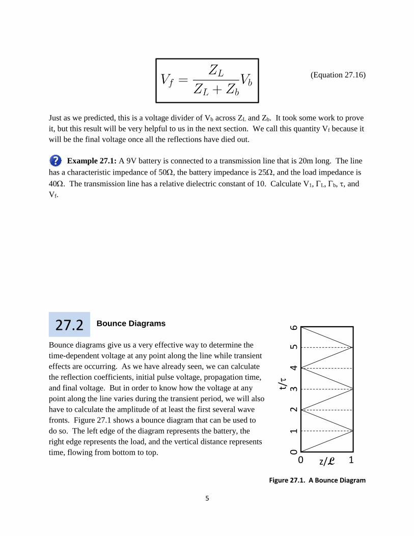
Example 27.1: A 9V battery is connected to a transmission line that is 20m long. The line

has a characteristic impedance of 50, the battery impedance is 25, and the load impedance is

40. The transmission line has a relative dielectric constant of 10. Calculate V1, L, b, , and

Vf.

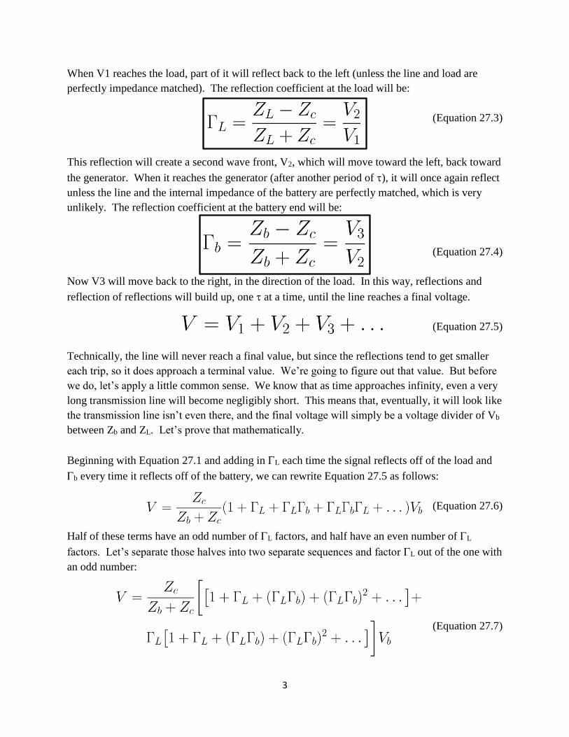
Bounce Diagrams

Bounce diagrams give us a very effective way to determine the

time-dependent voltage at any point along the line while transient

effects are occurring. As we have already seen, we can calculate

the reflection coefficients, initial pulse voltage, propagation time,

and final voltage. But in order to know how the voltage at any

point along the line varies during the transient period, we will also

have to calculate the amplitude of at least the first several wave

fronts. Figure 27.1 shows a bounce diagram that can be used to

do so. The left edge of the diagram represents the battery, the

right edge represents the load, and the vertical distance represents

time, flowing from bottom to top.

Figure 27.1. A Bounce Diagram

27.2

t/

01

23

45

6

z/L0 1

6

We can label the reflection coefficients at the left and right edge of the diagram, and each of the

diagonal lines represents a wave front, either moving toward the load or back toward the battery.

The voltage at any point along the line (say, at the middle) will simply be the sum of all the

voltages that have passed it at a particular time.

Example 27.2: Complete a bounce diagram for the situation in Example 27.1 and sketch

the voltage at the midpoint of the line from t=0 to t=6.

Notice that the voltage in this sketch approaches the value of Vf calculated in Example 27.1.

Special attention must be paid if the point being considered is at the load. In this case, the

voltage will include the incoming voltage, but it will not include the reflected voltage that just

left the load end. This voltage will be included in the plot once it has gone down to the battery

and come back to the load, so each transition in the voltage at the load end (after the first) will

include two new wave fronts. In all other ways, the problem is easier at the load end, since fewer

transitions in the voltage will need to be considered. Jest don’t include the reflected wave front

until it has gone all the way back to the battery and returned to the load.

Example 27.3: Perform the necessary calculations, draw a bounce diagram, and sketch the

voltage at the load for a setup in which the battery voltage is 100V, the battery internal

impedance is 100, the line impedance is 50, the load impedance is 30, the line has a relative

dielectric constant of 5, and the line length is 200m.

t/

01

23

45

6

z/L0 1 0 2 3 4 5 6

1V

2V

3V

4V

5V

6V

7

Again, notice how the voltage in the sketch approaches the value of Vf. This can be used to help

check your work and ensure you have not made any errors along the way.

Transient Effects: Pulse Propagation

We can also consider what happens when we send a narrow pulse down the transmission line. In

this case, “narrow” is defined as having a duration much less than the time it takes the signal to

propagate down the line:

(Equation 27.17)

Once again, the amplitude of the initial pulse can be calculated by a voltage divider of the

generator voltage Vg across the line impedance Zc and the generator impedance Zg:

27.3

t/

01

23

45

6

z/L0 10 2 3 4 5 6

6V

12V

18V

24V

30V

36V

8

(Equation 27.18)

We also know from intuition that when this narrow pulse reaches the load impedance, some of it

will be absorbed or transmitted, and some if it will probably be reflected. In this case, what we

really care about is the fraction of the pulse that is transmitted to the load, which is probably

either an antenna or another transmission line with a different characteristic impedance.

One rule that is universally true is the conservation of energy, so let’s begin there. We know that

energy is power multiplied by time, and the incoming energy must be equal to the reflected

energy plus the absorbed energy, so we can write:

(Equation 27.19)

The pulse durations will cancel out, and the power of each pulse can be written as the square of

the voltage divided by the impedance. Thus, we can rewrite Equations 27.19 as:

(Equation 27.20)

Substituting what we know for the reflection coefficient, we find:

(Equation 27.21)

Solving this equation for VL gives:

(Equation 27.22)

Factoring out common terms yields:

(Equation 27.23)

9

Establishing a common denominator under the square root gives:

(Equation 27.24)

Expanding the numerator and canceling wherever possible, we find:

(Equation 27.25)

Simplifying this result gives:

(Equation 27.26)

We can define the transmission coefficient to be the fraction of the initial pulse voltage that is

absorbed by the load:

(Equation 27.27)

As before, we can also write the reflection coefficient knowing that the following relationship is

true:

(Equation 27.28)

This can be written as follows:

(Equation 27.29)

Which can be simplified to:

(Equation 27.30)

Finally revealing:

10

(Equation 27.31)

It is reassuring that we obtain this same equation for the reflection coefficient, even though the

details of this circumstance are quite different, and we used a different method (conservation of

energy) to derive it this time.

Example 27.4: A narrow pulse is propagating along a line with characteristic impedance of

50, and it comes to a connection with a line of characteristic impedance 100. If the initial

pulse has an amplitude of 12V, what will be the amplitude of the reflected and transmitted pulse?

Example 27.5: Verify that energy is conserved in the situation described in Example 27.4.

Time Domain Reflectometry

As we have just shown, when a narrow pulse encounters any sort of obstacle or discontinuity,

part of it will be reflected back to the generator. We can use this to detect any sort of unexpected

condition on a transmission line using a method called Time Domain Reflectometry (TDR).

We simply send out a narrow pulse and then listen carefully to see if any reflections come back.

When they do, we know that the time that elapsed between the initial pulse and the reflection

27.4

11

represents the “time of flight” from the generator to the discontinuity and then back again. This

can be written as follows:

(Equation 27.32)

Since what we usually care about is the distance to the problem, we can solve this equation for d:

Thus, a simple test can be used not only to detect that there is a problem with the line, but it can

also be used to pinpoint the location of that problem with a pretty high level of precision. Quite

often, this could be used, for example, to narrow down the break in an electric power line to

within the range between a particular pair of poles, which makes the repair team’s job much

simpler.

Example 27.6: Time-Domain Reflectometry is used to search for an unauthorized

connection to a cable TV line. The transmission line has a relative dielectric constant of 12, and

the reflection is detected after 74s. How far away is the unauthorized connection?

Summary

When a battery is suddenly connected to a transmission line with a switch, the initial pulse

has the following voltage and propagation time:

The pulse will reflect at both the load end and at the battery end with the following reflection

coefficients:

27.5

12

The final voltage, once all the reflections have died down, will be:

Bounce diagrams can be used to determine the time-dependent voltage on the line as a

function of time. The voltage at any point is the sum of all the wave fronts that have passed

that point. If the point being considered is at the load end, then it does not “see” the reflected

wave front until it has traveled to the battery end and back again.

If a narrow pulse is launched toward a load, the initial pulse amplitude will be:

When it reaches the load, the transmission and reflection coefficients will be:

We can use this reflection in a method called time domain reflectometry to determine the

distance to a discontinuity in the transmission line:

Here, T is the time between the launch of a narrow pulse and the reception of its reflection.