chapter 3: analysis of bivariate data - departamento...
TRANSCRIPT
Introduction to Statistics
Chapter 3: Analysis of bivariate data
1. Tabular and graphical methods:
Absolute and relative frequency tables
Marginal and conditional frequencies
Graphical representations
2. Numerical summary: Covariance
Correlation coefficient
Regression line
3. How data change over time: Time series
Characteristics of time series: trend, seasonal and stationary components
Index numbers

Introduction to Statistics
Motivation
In chapter 2, we studied the characteristics of a single variable.
However, in many situations we measure two or more variables at
the same time
Number of languages spoken and Province of birth
Population and Parliamentary seats in a community
As well as analyzing the variables individually, we wish to see
whether there is any relation between them.
Data (x1,y1), (x2,y2), …, (xN,yN)
Introduction to Statistics
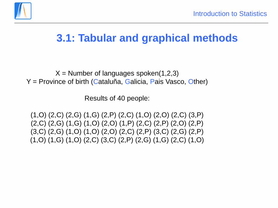
3.1: Tabular and graphical methods
X = Number of languages spoken(1,2,3)
Y = Province of birth (Cataluña, Galicia, Pais Vasco, Other)
Results of 40 people:
(1,O) (2,C) (2,G) (1,G) (2,P) (2,C) (1,O) (2,O) (2,C) (3,P)
(2,C) (2,G) (1,G) (1,O) (2,O) (1,P) (2,C) (2,P) (2,O) (2,P)
(3,C) (2,G) (1,O) (1,O) (2,O) (2,C) (2,P) (3,C) (2,G) (2,P)
(1,O) (1,G) (1,O) (2,C) (3,C) (2,P) (2,G) (1,G) (2,C) (1,O)

Introduction to Statistics
The two-way table
There are 3 Catalans who speak 3 languages.
X / Y C G P O
1 0 4 1 8
2 8 5 6 4
3 3 0 1 0
40
There are
40 people in
the sample
Introduction to Statistics
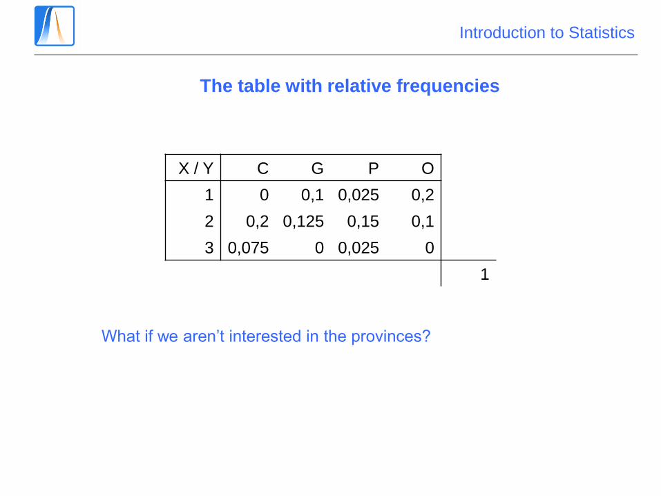
The table with relative frequencies
X / Y C G P O
1 0 0,1 0,025 0,2
2 0,2 0,125 0,15 0,1
3 0,075 0 0,025 0
1
What if we aren’t interested in the provinces?
Introduction to Statistics
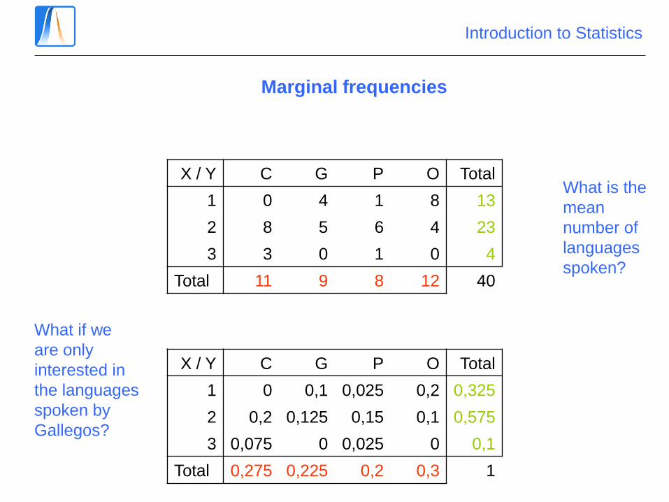
Marginal frequencies
X / Y C G P O Total
1 0 4 1 8 13
2 8 5 6 4 23
3 3 0 1 0 4
Total 11 9 8 12 40
X / Y C G P O Total
1 0 0,1 0,025 0,2 0,325
2 0,2 0,125 0,15 0,1 0,575
3 0,075 0 0,025 0 0,1
Total 0,275 0,225 0,2 0,3 1
What if we
are only
interested in
the languages
spoken by
Gallegos?
What is the
mean
number of
languages
spoken?
Introduction to Statistics
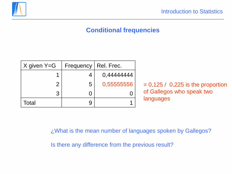
Conditional frequencies
X given Y=G Frequency Rel. Frec.
1 4 0,44444444
2 5 0,55555556
3 0 0
Total 9 1
= 0,125 / 0,225 is the proportion
of Gallegos who speak two
languages
¿What is the mean number of languages spoken by Gallegos?
Is there any difference from the previous result?
Introduction to Statistics
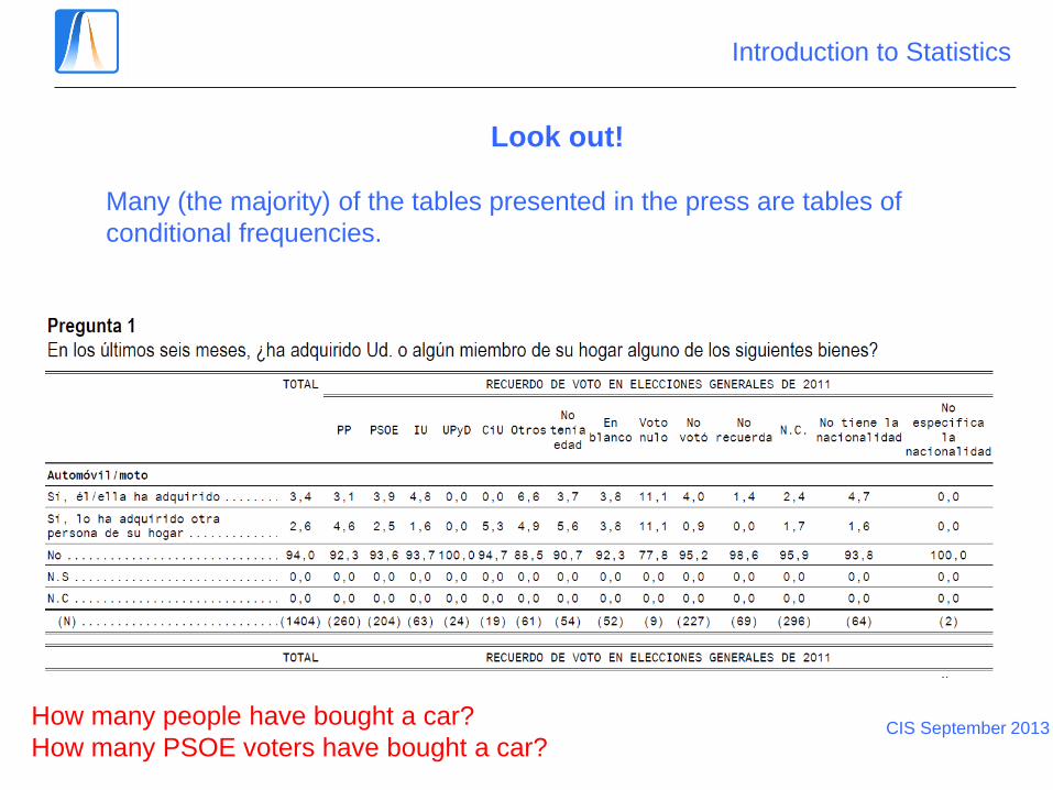
Look out!
Many (the majority) of the tables presented in the press are tables of
conditional frequencies.
How many people have bought a car?
How many PSOE voters have bought a car? CIS September 2013
Introduction to Statistics
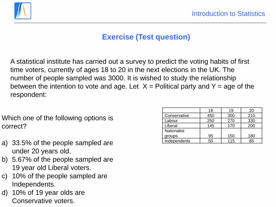
Exercise (Test question)
A statistical institute has carried out a survey to predict the voting habits of first
time voters, currently of ages 18 to 20 in the next elections in the UK. The
number of people sampled was 3000. It is wished to study the relationship
between the intention to vote and age. Let X = Political party and Y = age of the
respondent:
18 19 20
Conservative 450 300 210
Labour 250 270 330
Liberal 145 170 200
Nationalist
groups 95 150 180
Independents 50 115 85
Which one of the following options is
correct?
a) 33.5% of the people sampled are
under 20 years old.
b) 5.67% of the people sampled are
19 year old Liberal voters.
c) 10% of the people sampled are
Independents.
d) 10% of 19 year olds are
Conservative voters.
Introduction to Statistics
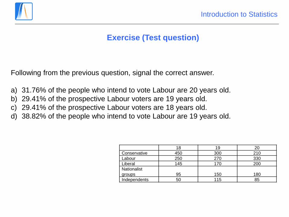
Exercise (Test question)
Following from the previous question, signal the correct answer.
a) 31.76% of the people who intend to vote Labour are 20 years old.
b) 29.41% of the prospective Labour voters are 19 years old.
c) 29.41% of the prospective Labour voters are 18 years old.
d) 38.82% of the people who intend to vote Labour are 19 years old.
18 19 20
Conservative 450 300 210
Labour 250 270 330
Liberal 145 170 200
Nationalist
groups 95 150 180
Independents 50 115 85
Introduction to Statistics
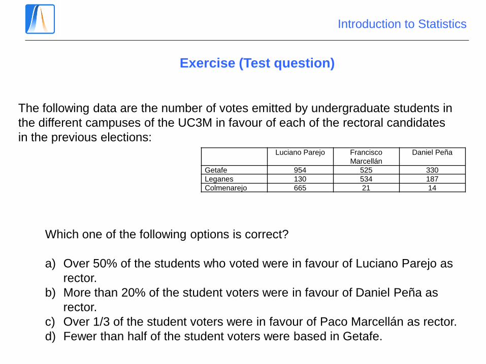
Exercise (Test question)
The following data are the number of votes emitted by undergraduate students in
the different campuses of the UC3M in favour of each of the rectoral candidates
in the previous elections: Luciano Parejo Francisco
Marcellán
Daniel Peña
Getafe 954 525 330
Leganes 130 534 187
Colmenarejo 665 21 14
Which one of the following options is correct?
a) Over 50% of the students who voted were in favour of Luciano Parejo as
rector.
b) More than 20% of the student voters were in favour of Daniel Peña as
rector.
c) Over 1/3 of the student voters were in favour of Paco Marcellán as rector.
d) Fewer than half of the student voters were based in Getafe.

Introduction to Statistics
Exercise (Test question)
Following from the previous question, signal the correct answer.
Luciano Parejo Francisco
Marcellán
Daniel Peña
Getafe 954 525 330
Leganes 130 534 187
Colmenarejo 665 21 14
a) Approximately 54.55% of the students in Getafe are in favour of Luciano
Parejo.
b) Approximately 54.55% of the students who voted for Luciano Parejo
come from Getafe.
c) Approximately 52.74% of the students who voted for Luciano Parejo
come from Getafe.
d) None of the above.
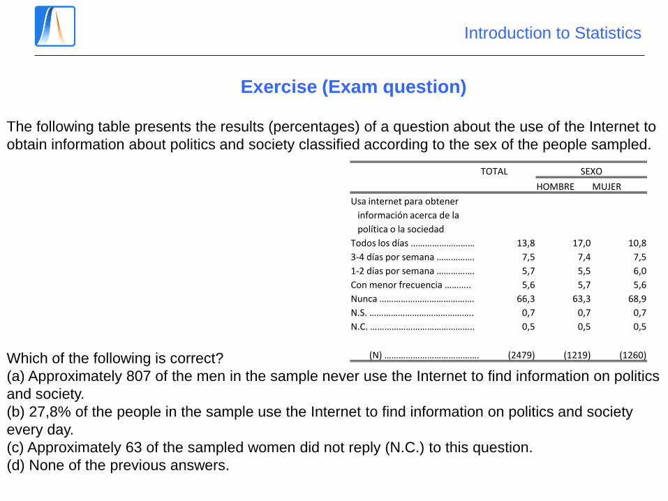
The following table presents the results (percentages) of a question about the use of the Internet to
obtain information about politics and society classified according to the sex of the people sampled.
Which of the following is correct?
(a) Approximately 807 of the men in the sample never use the Internet to find information on politics
and society.
(b) 27,8% of the people in the sample use the Internet to find information on politics and society
every day.
(c) Approximately 63 of the sampled women did not reply (N.C.) to this question.
(d) None of the previous answers.
Introduction to Statistics
Exercise (Exam question)
TOTAL SEXO
HOMBRE MUJER
Usa internet para obtener
información acerca de la
política o la sociedad
Todos los días ……………………… 13,8 17,0 10,8
3-4 días por semana ……………. 7,5 7,4 7,5
1-2 días por semana ……………. 5,7 5,5 6,0
Con menor frecuencia ……….. 5,6 5,7 5,6
Nunca …………………………………. 66,3 63,3 68,9
N.S. …………………………………….. 0,7 0,7 0,7
N.C. …………………………………….. 0,5 0,5 0,5
(N) …………………………………. (2479) (1219) (1260)
Introduction to Statistics
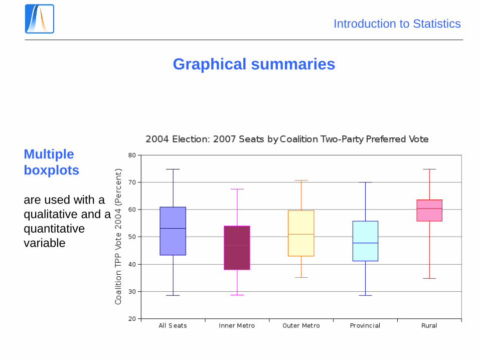
Graphical summaries
Multiple
boxplots
are used with a
qualitative and a
quantitative
variable
Introduction to Statistics
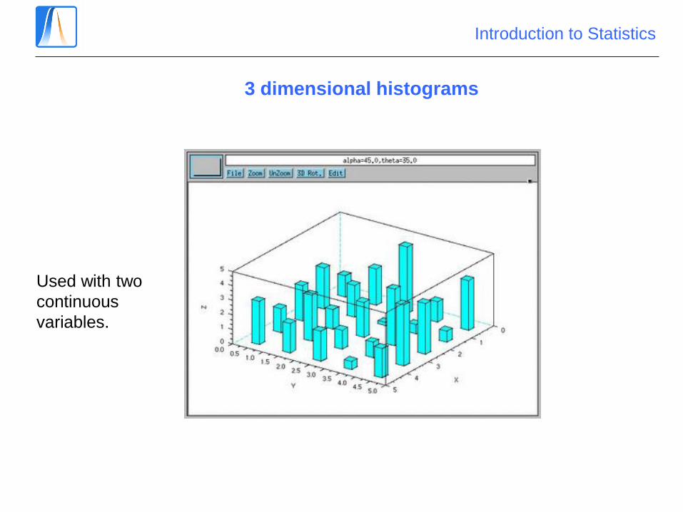
3 dimensional histograms
Used with two
continuous
variables.
Introduction to Statistics
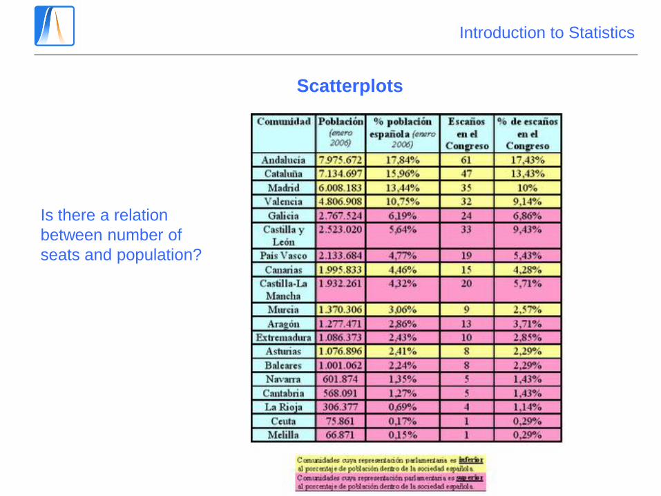
Scatterplots
Is there a relation
between number of
seats and population?
Introduction to Statistics
0
20
40
60
80
0 2E+06 4E+06 6E+06 8E+06 1E+07
Población
Escañ
os
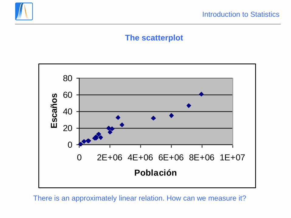
There is an approximately linear relation. How can we measure it?
The scatterplot
Introduction to Statistics
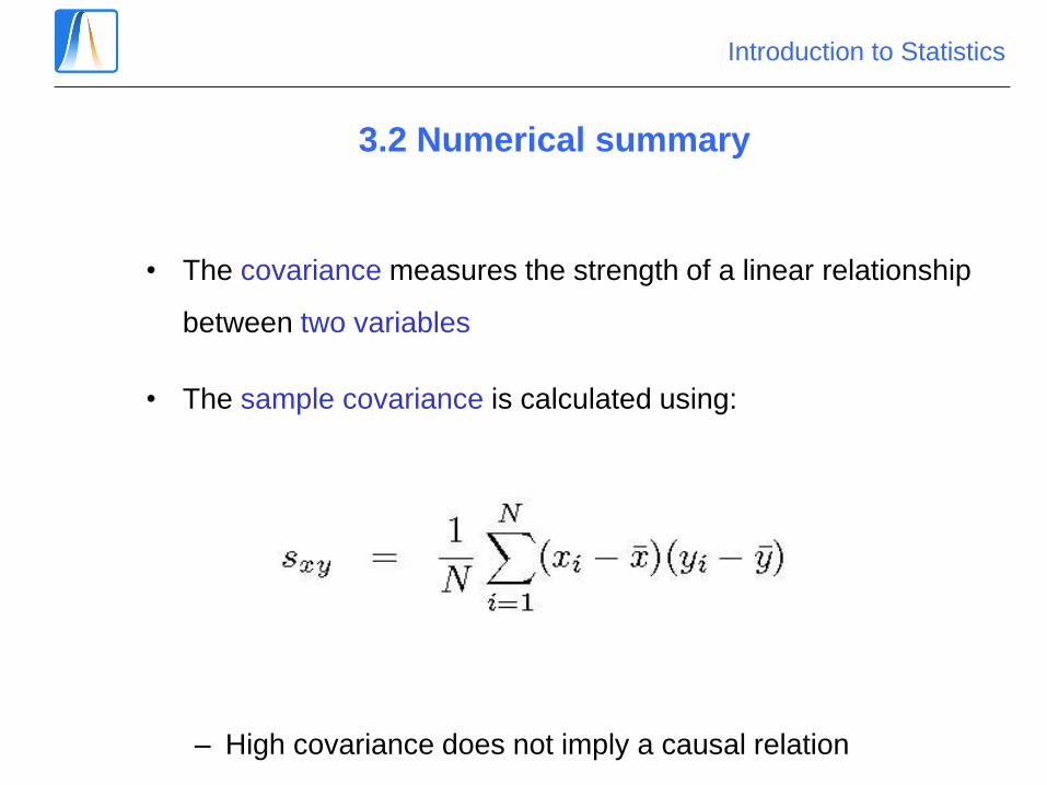
• The covariance measures the strength of a linear relationship
between two variables
• The sample covariance is calculated using:
– High covariance does not imply a causal relation
3.2 Numerical summary
Introduction to Statistics
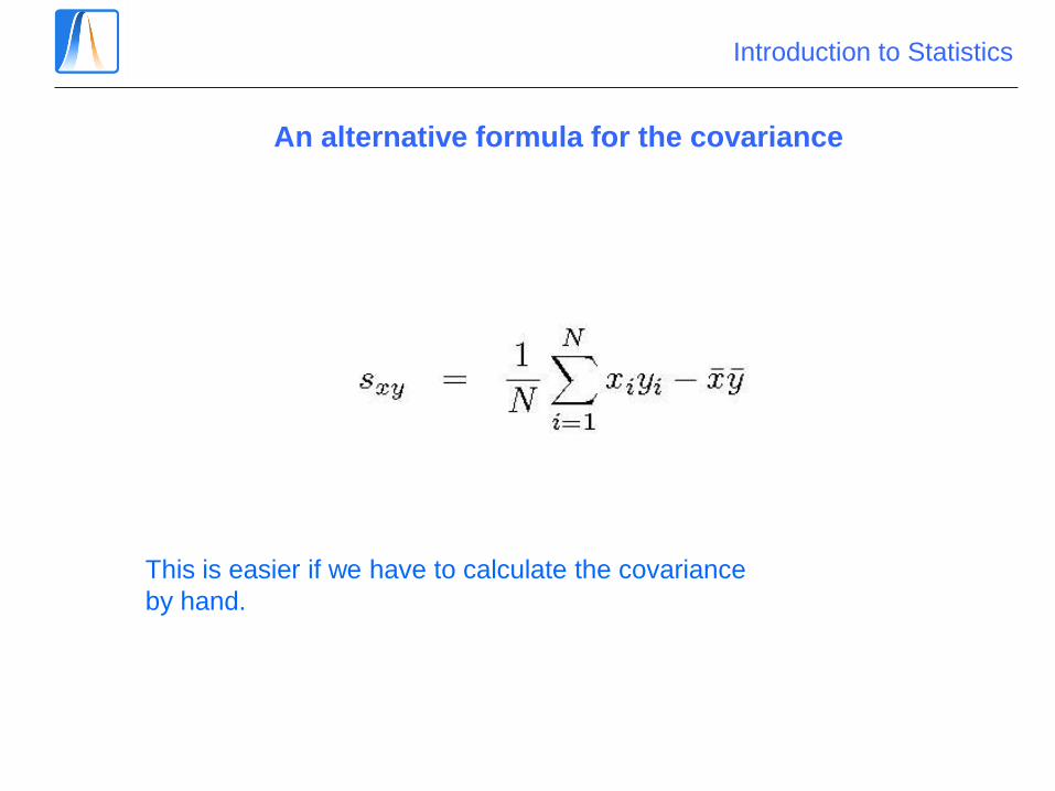
An alternative formula for the covariance
This is easier if we have to calculate the covariance
by hand.
Introduction to Statistics
Interpretation of the covariance
Cov(x,y) > 0: X and Y tend to move in the same
direction
Cov(x,y) < 0: X and Y tend to move in opposite
directions.
Cov(x,y) = 0: There is no linear relation between X and
Y.
Introduction to Statistics
Disadvantage of the covariance
In our example, the covariance is about 36043027,5. Does
this show a strong relationship or not?
What are the units of the covariance?
How can we correct the problem?
Introduction to Statistics
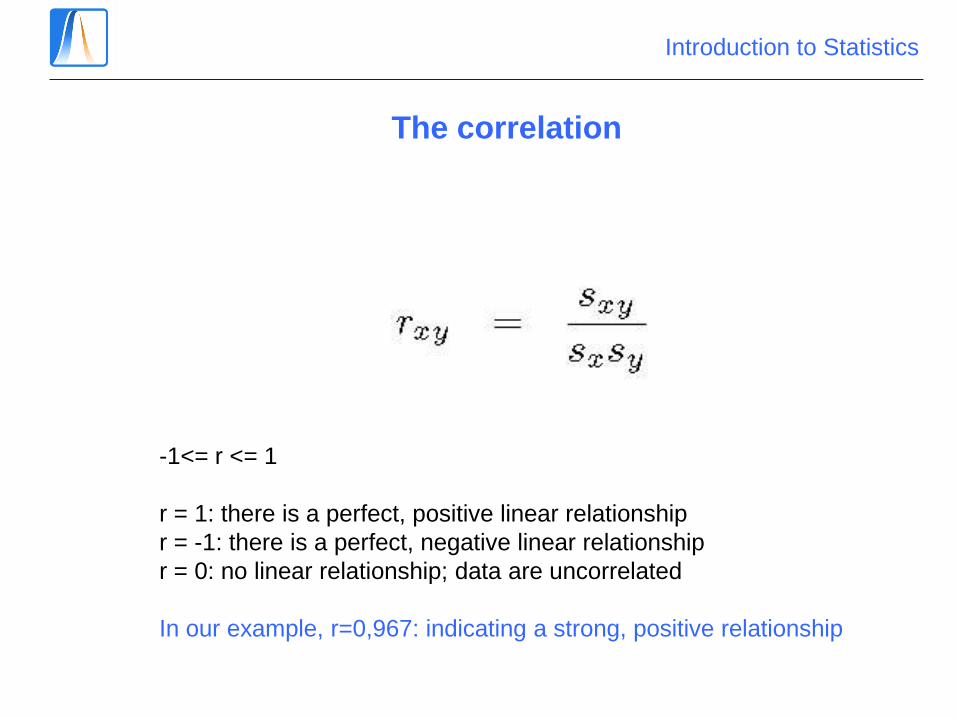
The correlation
-1<= r <= 1
r = 1: there is a perfect, positive linear relationship
r = -1: there is a perfect, negative linear relationship
r = 0: no linear relationship; data are uncorrelated
In our example, r=0,967: indicating a strong, positive relationship
Introduction to Statistics
Y
X
Y
X
Y
X
Y
X X
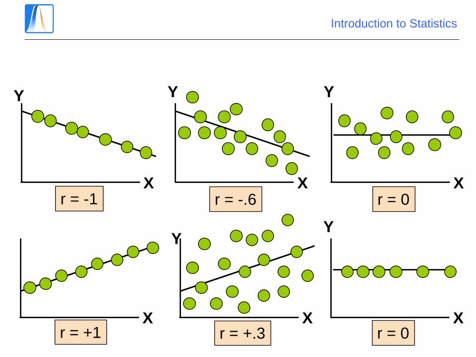
r = -1 r = -.6 r = 0
r = +.3 r = +1
Y
X r = 0
Introduction to Statistics
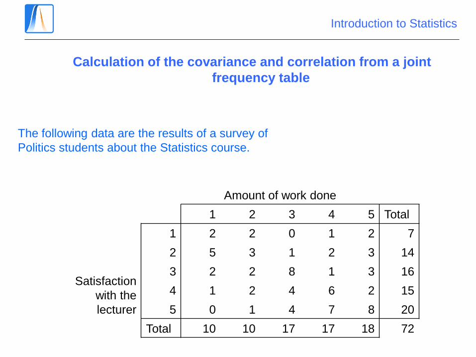
Calculation of the covariance and correlation from a joint
frequency table
Amount of work done
1 2 3 4 5 Total
Satisfaction
with the
lecturer
1 2 2 0 1 2 7
2 5 3 1 2 3 14
3 2 2 8 1 3 16
4 1 2 4 6 2 15
5 0 1 4 7 8 20
Total 10 10 17 17 18 72
The following data are the results of a survey of
Politics students about the Statistics course.

Introduction to Statistics
Calculate the table of relative frequencies …
Work done
1 2 3 4 5 Total
Satisfaction
1 0,028 0,028 0,000 0,014 0,028 0,097
2 0,069 0,042 0,014 0,028 0,042 0,194
3 0,028 0,028 0,111 0,014 0,042 0,222
4 0,014 0,028 0,056 0,083 0,028 0,208
5 0,000 0,014 0,056 0,097 0,111 0,278
Total 0,139 0,139 0,236 0,236 0,250 1,000
… and the marginal means
1 2 3 4 5
0,139 0,139 0,236 0,236 0,250
0,139 0,278 0,708 0,944 1,250 3,319
1 0,097 0,097
2 0,194 0,389
3 0,222 0,667
4 0,208 0,833
5 0,278 1,389
3,375
Introduction to Statistics
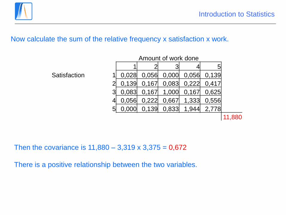
Now calculate the sum of the relative frequency x satisfaction x work.
Amount of work done
1 2 3 4 5
Satisfaction 1 0,028 0,056 0,000 0,056 0,139
2 0,139 0,167 0,083 0,222 0,417
3 0,083 0,167 1,000 0,167 0,625
4 0,056 0,222 0,667 1,333 0,556
5 0,000 0,139 0,833 1,944 2,778
11,880
Then the covariance is 11,880 – 3,319 x 3,375 = 0,672
There is a positive relationship between the two variables.
Introduction to Statistics
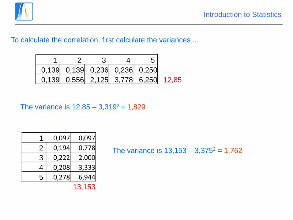
To calculate the correlation, first calculate the variances ...
The variance is 13,153 – 3,3752 = 1,762
1 2 3 4 5
0,139 0,139 0,236 0,236 0,250
0,139 0,556 2,125 3,778 6,250 12,85
The variance is 12,85 – 3,3192 = 1,829
1 0,097 0,097
2 0,194 0,778
3 0,222 2,000
4 0,208 3,333
5 0,278 6,944
13,153
Introduction to Statistics
Finally, divide the covariance by the product of the square roots of the
variances to calculate the correlation.
The result is 0,374.
There is a slight positive relationship between the two variables.