sectoring, splitting, and micro-cell zone concept are also discussed to improve the

capacity of a cellular system by increasing S/I. The major objective of these methods is to

increase the number of subscribers in a system.

Chapter 3

Channel Allocation and Multi-agent System: A

Literature Survey

3.1Introduction

Though there has been a remarkable increase in the mobile user population, the narrow

radio spectrum allocated for communication is limited. The channel allocation aims to

allocate number of channels to each cell in such way that maximum frequency spectrum

utilization takes place and interference is minimized. In this chapter various schemes that

are used to allocate channels to the cells are reviewed and performance of each of these

schemes is discussed.

3.2The Channel Allocation Problem

The Channel Allocation Problem has two aspects [80]:

i. Frequencies are allocated to a pair of wireless communication connections in such

a way that data transfer between every connection is possible. The frequencies must

be selected from a pre-specified set and different frequencies should be allocated to

each connection. For bidirectional traffic, two frequencies should be selected one for

each direction.

ii. The frequencies allocated to different connections may interfere with each other

resulting in a loss of signal quality. The following two conditions must be satisfied

for interference to take place:

a) The frequencies must either be close on the electromagnetic band or

harmonics of one another. However, latter effect is very limited.

44

b) The two interfering connections must be very close to each other. The

interfering signals must have similar energy levels at the positions where they

may disturb each other.

The radio frequency band [fmin, fmax] provided to service provider is generally partitioned

in a set of channels, and all the channels are having same bandwidth δ of frequencies.

The channels are generally numbered from 1 to N, where N = (fmax - fmin)/ δ and the

existing channels are denoted by the domain D = {1, . . . , N}. It may happen that not all

the channels from a domain D are available for a particular connection. The channels

available for a particular connection v form a subset Dv ∈ D and information can be

transmitted from transmitter to receiver on each available channel. Two channels are

required for bidirectional communication, one for each direction. The second channel is

always ignored n the models considered in the literature. Instead of using one band [fmin,

fmax], most of the applications use two bands [f1min, f1

max] and [f2min, f2

max] of N channels:

one with the channels {1, . . . , N}, and another with the channels {s + 1 , . . . , s + N},

where s >> N. Therefore, the backward connection uses a channel which is shifted s

channels up in the frequency domain. The s should be chosen in such way that backward

channels do not interfere with the forward channels. As a result, every allocation for the

forward channels can directly be transformed to an allocation for the backward channels

with comparable performance.

Interference of signals at the receiver is measured by the signal-to-noise ratio or signal-

to-interference ratio. Therefore, the transmitted signal must be clearly understandable.

The noise generally comes due to the presence of other signals using same as well as

adjacent frequencies. There may be more than one sources present in the area that

transmits on the same or a close frequency and, therefore, contribute to the noise at the

receiver. In practical conditions, a threshold value of around 15 dB is found acceptable

for the signal-to-noise ratio. The calculation of the interference level is a hard job, since it

not only depends on the choice of signal and its strength, but also on the environment. If

the environment factor is ignored and considers only the signals transmitted at the same

frequency channel, then the interference at the receiver is computed with the following

formula:

45

P/dγ

where P is the transmitter power and d is the distance to the troubled receiver, whereas, γ

is a fading factor ( 2 ≤ γ ≤ 4). If the interfering signal is transmitted on a frequency, which

is present at a distance of n ≥ 1 units of the original signal, then a filtering factor of -15(1

+ log2n) is also taken into consideration [139]. The fact that the presence of multiple

signals in the area may disturb communication quality, is overlooked in most of the

models. A prominent exception is given by Fischetti et al., in which in order to determine

the interference of neighboring connections, some constraints are developed and another

assumption is the calculation of the levels of interference [124].

The two-way traffic creates several problems, as interference may not be symmetric: if a

transceiver pair (t1, t2) transmitting on frequencies f and (f + s) from t1 to t2, and another

transceiver pair (s1, s2) transmitting on frequencies g and (g + s) where f and g interfere,

(f + s) and (g + s) interfere, the amount of interference at t1 and t2 may be different

because these transceivers may possibly be having different distances from s1 and s2. This

aspect is also overlooked by most researchers.

Based on the application, one or multiple connections may be set between the same end

points. Therefore, this is modeled by assuming that (cz ∈Z+) frequencies are allocated to

connection v. Therefore, with the introduction of an extra value for certain combination

of frequencies (f,g ∈ D), the interference between frequencies allocated to the same

connection can only be avoided. In practical conditions and based on the demand for

connections, the value cz may vary with time. Through this property, the methods

suggested to deal with the channel allocation problem can be divided into three

categories: Fixed Channel Allocation (FCA), Dynamic Channel Allocation (DCA), and

Hybrid Channel Allocation (HCA).

In FCA, radio channels are allocated to each connection in advance and allocation is

based on the forecasted demand. Therefore, in order to satisfy the demand for

connections the radio channel allocation is not allowed to change on-line. Whereas, in

DCA schemes frequencies are allocated on-line to the wireless connections in such a way

46

that the actual demand is met and the interference is minimized. An example of a

procedure for DCA is presented by Janssen [85], who discussed the fixed preference

assignment scheme for DCA. According to this paper, for every cell a preference list of

frequencies exist to meet the demand and the preference lists must be created in such a

way, so that it should be optimal according to some performance measure.

Finally, HCA scheme is a combination of FCA and DCA and is implemented to get an

enhanced overall performance of the network. In HCA schemes some of the frequencies

are allocated to every connection beforehand, whereas rest of the frequencies can be used

for on-line allocation upon request. An example of an HCA scheme is given by

Sandalidis et al., who describe the neural network and genetic algorithm methods for

channel borrowing in order to solve the channel allocation problem [76]. In this scheme,

frequencies are allocated permanently to the connections. However, when the demand for

frequencies exceeds the number of frequencies available in the area, the connection can

borrow an unused frequency allocated to an adjacent connection. The performance of

networks that work on DCA and HCA schemes is generally studied via simulation of the

part time methods. It is also proved by Johri [153] that DCA schemes perform better than

FCA schemes under light traffic and non-uniform traffic loads. However, FCA schemes

perform better than DCA under uniform and heavy load. Katzela and Naghshineh [80]

provided a survey on the topic of FCA, DCA and HCA schemes.

3.3Fixed Channel Allocation

In FCA, fixed numbers of radio channels are allocated to each connection based on the

expected load. The standard representation of a CAP is by means of a graph G = (V,E),

where V is the vertices and E is the edges of the graph, also called the interference graph

or constraint graph. Each connection is represented by vertex v ∈ V. The available

channels for a vertex are denoted by the set Dv ⊆ D. Ci denote the number of frequencies

or channels required for connection v ∈ V. Two vertices v and w for which the

corresponding connection may interfere for at least one pair of frequencies, are connected

by an edge {v,w} ∈ E. For each pair of frequencies f ∈ D, and g ∈ D, the combined

47

choice of frequencies is penalized by a measure depending on the interference level and

pvwfg the penalty. The interference between frequencies f ∈ D, and g ∈ D, allocated to the

same vertex v can be represented in the same way: an edge {v, v} ∈ E and penalty pvvfg.

This can also be modeled in a different way, replacing v and cv vertices and additional

edges between them. In order to reduce the interference, some instances to deal with a

frequency plan are considered, and this reduction in interference happens under minimum

changes of the total frequency plan, therefore, changes in the frequency plan are also

penalized per change. This is modeled with extra penalties imposed on the frequencies to

be selected for each vertex: the choice of frequency f ∈ Dv costs qvf.

Various methods to solve the CAP can be subdivided into two main steams and

frequencies are allocated to each vertex in such a way that either the maximum penalty

incurred by a solution (minmax) is minimized or total penalty incurred by the solution

(minsum).

3.3.1 Minimization of the Maximum Penalty

Instead of calculating a solution where the maximum penalty is minimized [194], [26], a

solution is searched where the incurred interference does not go beyond a given threshold

value. Therefore, certain frequencies and combinations of frequencies are not allowed.

This basically reduces the penalty matrices of the edges to 0, 1 matrices. Frequency

combinations with penalty 0 are allowed, whereas, penalty 1 is not allowed. Therefore,

the objective here is to find a feasible solution, i.e. a solution in which no prohibited

frequency combinations are selected. If such an allocation is present, a second objective

can be introduced. The second objective introduces a preference relation between all

feasible allocations. Therefore, the problem of minimizing or reducing the number of

used frequencies is called the minimum cardinality problem, or minimum order problem.

The objective in this case is to reduce or minimize the span, i.e., the difference between

the highest and lowest frequencies are selected.

If the incurred penalties go above the given threshold value in every allocation, two

solutions are possible. In the first solution, the threshold value can be increased for

48

allowing allocation with greater interference and the other solution is that, the partial

allocation can be searched that does not go over the set threshold penalty. Therefore, the

objective here is minimization of the blocking probability. If in any case mv frequencies

can be allocated to a connection instead of the requested cv frequencies, the probability to

reject a connection can be computed. This probability is called the blocking probability.

Optimal partial allocations can minimize or reduce the overall blocking probability of the

network.

3.3.2 Minimization of the Cumulative Penalty

The minsum method is not commonly seen in practical situations, but in some cases it is

linked with the minmax criterion by introducing the threshold values for penalties that

indicate the maximum acceptable interference. Then the feasible solutions are looked

with a minimum total penalty and no penalty should go beyond the threshold value. For

describing real-world problems, this combined form is found to be most exact, but it is

also the one, for which determining an optimal solution is very difficult.

Four different models to solve the CAP are:

(i) Minimum Order Channel Allocation Problem (MO-CAP)

(ii) Minimum Span Channel Allocation Problem (MS-CAP)

(iii) Minimum Blocking Channel Allocation Problem (MB-CAP)

(iv) Minimum (Total) Interference Channel Allocation Problem (MI-CAP)

3.3.3 Channel Allocation and Graph Coloring

The minmax criterion is strongly linked to generalized coloring problems e.g. T-coloring

or list coloring and this relation have been first explained by Metzger [26] and Hale

[194]. The relation of looking a feasible solution with graph coloring, is due to two basic

modeling aspects: first, the levels of interference (in acceptable and unacceptable levels),

reduces the problem to prohibited combinations and permitted combinations similar to

graph coloring problem, where two adjacent vertices are not allowed to color, with the

same color. Second, in many cases the interference levels are associated with the distance

49

between the allocated frequencies: the smaller the distance between two allocated

frequencies, the larger is the interference level pvwfg. Therefore, interference between the

connections v and w is defined unacceptable if f ∈ Dv and g ∈ Dw are located at a

distance lesser than dvw of each other. The interference is acceptable if the radio

frequencies distance, i.e., | f – g | ≥ dvw is large. Now, if the problem is relaxed by setting

all dvw = 1 for {v, w} ∈ E, which is not far away from reality, then equal choices of

frequencies are penalized for connected vertices. Therefore, frequencies are viewed as

colors, and a solution should have very few edges for which the end vertices are allocated

the same colors.

In a more general setting, it is not permitted to allocate frequencies that is different from

a value contained in a set Tvw (containing 0), i.e., |f - g| ∉ Tvw and if Tvw is defined by

{0,...., dvw - 1} then the problems are alike. However, more general sets with non-

consecutive numbers can also be defined e.g. in UHF television broadcasting the set Tvw

contains non-successive set of integers [194]. If all sets Tvw are, then the problem is

reduced to a T-coloring problem, as introduced by Hale [78]. He properly defined both

minimum span and minimum order variants of T-coloring problem, and linked them to

the channel allocation problem.

Another method to represent the minimum distance constraints is through the use of a

compatibility matrix C, where the rows and columns of the matrix correspond to the

connections. The values Cvw = dvw indicate the minimum frequency separation distance. In

case Cvw = 0, v and w are not adjacent vertices, and no constraint on the allocated

frequencies exists and the constraints are differently depending on the value of Cvw. The

co-channel, adjacent-channel, and co-site constraints can be differentiated based on the

values of Cvw. The co-channel and adjacent-channel constraints are commonly used to

define a difference between values, if Cvw = 1 (same frequencies cannot be allocated to

both the connections), and if Cvw ≥ 2 (adjacent channels cannot be allocated to the

connections), respectively.

3.4Minimum Order Channel Allocation Problem

50

In the minimum order channel allocation problem (MO-CAP), radio channels are

allocated in such a way that no intolerable interference occurs, and the number of

different used frequencies for a particular connection is minimized. Therefore, the

problem can be described as follows:

INSTANCE: Undirected graph G = (V, E), {v,v}∈ E, for all v ∈ V, sets Tvw ⊂ Z, {v, w}

∈ E, 0 ∈ Tvw demand cv ∈ Z+, domain subsets Dv ⊆ Z+ for all v ∈ V, D = Uv∈VDv, and

positive integer K.

QUESTION: Find the minimum order allocation of subsets f : V → 2D such that,

(i) )(vf = cv,

(ii) F(v) ⊆ Dv,

(iii) ∉− gf Tvw,

(iv) U v∈V )(vf ≤ K?

The MO-CAP is the first frequency allocation problem that was discussed in the

literature. According to Hale [194], Metzger [26] has brought this problem into the notice

of operations research society. Therefore, MO-CAP is a clear generalization of the graph

coloring problem.

According to Garey and Johnson [131] Graph K-Colorability is:

INSTANCE: Undirected graph G = (V, E), and positive integer K ≤ |V|.

QUESTION: Is G a K-colorable graph, i.e., does there exist a function f : V → {1,2,.., K}

such that fu ≠ fw whenever {u, w} ∈ E?

Minimum number of colors required to color the graph is expressed as χ (G)- and it is

proved by Karp that Graph K-Colorability problem is NP-complete for all K > 3 [162].

As a result, MO-CAP is NP-complete as well. Garey and Johnson proved that within a

factor 2 approximation of the optimal value is NP-complete as well [130]. Hale proposed

a generalization of graph coloring and is therefore, known as T-coloring [194].

Minimum Order T-Coloring Problem as explained by (Hale [194]) is:

51

INSTANCE: Undirected graph G = (V,E), set T ⊂ Z+, {v, w} ∈ E, 0 ∈ T, and positive

integer K.

QUESTION: Does there exist an allocation f : V → Ζ + such that, fv - fw∉ T for all

{v, w} ∈ E and Uv∈V Fv ≤ K?The minimum number of colors required to color a graph G with respect to a set T is

denoted by χ Τ (G). Cozzens and Roberts have proved that χ Τ (G) = χ (G): Let (fv)v∈V

be a coloring for G, and let (tmax = maxt∈T t+1). Then the coloring (tmaxfv) v∈V is a feasible

T-coloring [39].

As a result, research in this direction has largely been focused on the graph coloring

problem in place of the T-coloring problem, or on the minimum span T-coloring

problem.

Another generalization of graph coloring problem is the List Coloring Problem.

Therefore, Minimum Order List Coloring Problem according to Erdos et al. [152], and

Vizing [192] is:

INSTANCE: Undirected graph G = (V, E), subsets Dv ⊂ Z+ (lists) for all v ∈ V, D = Uv

∈VDv, and positive integer if.

QUESTION: Does there exist an allocation of subsets f : V → D such that,

(i) fv ∈ Dv,

(ii) fv ≠ fw for all {v, w} ∈ E and,

(iii) Uv∈V F(v) ≤ K?

The Minimum Order List Coloring Problem is NP-complete, even for special purpose

graphs the graph coloring problem may be solved in linear time, e.g. for interval graphs

[121].

52

For the common MO-CAP, Aardal et al. [107] has presented an integer linear

programming formulation. For each vertex v and offered frequency f, a binary variable is

introduced:

∈

=

otherwise 0

vertex toassigned is D ffrequency if 1 v

vxvf

Moreover, a binary variable yf denotes the use of frequency f :

∈

=

otherwise 0

sed is D ffrequency if 1

uyf

Then, MO-CAP reads

min ∑∈Df

fy (3.1)

s.t. vc =∑∈Dvf

vfx V ∈∀v (3.2)

xvf + xwg ≤ 1 { } wv Dg DfEwv , , , ∈∈∈∀( ) ( ) ( )( )wvgfTgf vw - ≠∨≠∧∈ (3.3)

xvf ≤ yf vDfVv , =∈∀ (3.4)xvf = {0, 1} vDfVv , =∈∀ (3.5)yf = {0, 1} ∀ Df ∈ (3.6)

The constraints (3.2) model that cv frequencies have to be allocated to connection v ∈ V.

The constraints (3.3) modeled the prohibited set of frequencies, whereas (3.4) specifies

that if the resultant frequency is used by the allocation the variable y is set to. The goal

(3.1) just sums the use of the existing frequencies.

3.4.1 Lower Bounds and Exact Methods

In the CALMA project, Aardal et al. [107] had used integer programming techniques to

solve the problem. Cutting planes were added by them to the formulation (3.1)-(3.6). For

related vertex packing problem, the used cutting planes are very well known suitable

inequalities. Extra preprocessing techniques and particular branching strategies have

actually made it feasible to solve large instances (up to 916 vertices) to optimality. For all

53

the examined instances, optimal values were proved in this way. The lower bounds based

on linear programming (LP) were compared with bounds obtained through combinatorial

arguments like cliques in the coloring number (col.), and the generalized coloring (gcol.).

In all the 4 cases, the linear programming (LP) provided the best bound.

Hurkens and Tiourine calculated minimum order lower bounds of any allocation [36]. In

the constraint graphs, the lower bounds were obtained through the detection of cliques.

The clique lower bound can be enhanced by the combination of the information about

several cliques.

Finally, Kolen et al. applied the constraint satisfaction techniques to the MO-CAP [14].

The optimal solution is reported only for two instances by the combination of lower and

upper bounds created by the proposed technique.

3.4.2 Heuristics

Most of the heuristics for MO-CAP were proposed in the CALMA project. Besides lower

bounding techniques, Tiourine, Hurkens, and Lenstra [36][170] have also applied local

search techniques, e.g. simulated annealing (SA), variable depth search (VDS), and tabu

search (TS) [171]. Tabu search was applied by a group from King's College London as

well [2] [1]. As compared to the tabu search approach, the neighborhood function is less

sophisticated [170]. Moreover, Bouju et al. also applied a General NETwork algorithm

(GENET) for constraint satisfaction problems to the same instances [1]. They got optimal

or near optimal solutions.

A potential reduction (PR) algorithm for the MO-CAP was introduced by Warners et al.

[92] [91]. The algorithm is motivated by Karmarkar's interior point potential reduction

method for combinatorial optimization problems ([13], [141], [142]). Pasechnick [42]

enhanced the performance of the algorithm, and the optimal values of the instance

GRAPH 14 were proved.

Genetic algorithm was applied to the instances by Kapsalis et al. [4]. The obtained results

are found less satisfactory than the other algorithms, and the optimal solutions have been

54

obtained only for two instances. Crisan et al. [31] applied evolutionary search (ES) to

MO-CAP. Evolutionary search performs the repetitive mutation of a solution according

to a certain mutation operator. The performance of an evolutionary search algorithm was

investigated on a CALMA instance, and the search space was analyzed in order to get

some information on the difficulty of the instances. They found that there is very less

association between two good frequency allocation plans, than between two good tours in

the traveling salesman problem. This shows that local search techniques will encounter

more difficulties to arrive at the optimum solution for MO-CAP, than similar heuristics

for the traveling salesman problem. Their results with evolutionary search are similar

with the results of simulated annealing, tabu search, and variable depth search [170].

Finally, a genetic algorithm approach was applied by Cuppini [122] to the minimum

order problem. As compared to the other genetic algorithms for CAPs, an allocation is

represented by |D| genes of N = ∑ ∈VvvC elements (in the majority genetic algorithms |

V| genes of size |Dv| are used to represent an allocation).

3.5 Minimum Span Channel Allocation Problem

In the minimum span channel allocation problem (MS-CAP), the problem is to allocate

frequencies in such a way that no intolerable interference should occur, and the difference

between the maximum and minimum used frequency (the span), is minimized [194].

Therefore, the problem has been described as follows:

INSTANCE: Undirected graph G = (V, E ) , {v, v} ∈ E, for all v ∈ V, sets Tvw ⊂ Z,

{v, w} ∈ E, 0 ∈ Tvw, demand cv ∈ Z+, domain subsets Dv, ⊆ Z+ for all v ∈V, D = Uv∈

VDv and positive integer K.

QUESTION: Does there present an allocation of subsets f : V → 2D such that,

(i) )(vf = cv,

(ii) F(v) ⊆ Dv,

(iii) ∉− gf Tvw for all {v, w} ∈ E, f ∈ f(v), g ∈ f(w), v ≠ w or f ≠ g , and

(iv) max Uv∈VF(v) – min Uv∈VF(v) ≤ K?

55

The problems MO-CAP and MS-CAP are comparable [194], if Dv = Z+ and Tvw = {0}.

However, there exist examples in which neither a minimum order allocation with

minimum span, nor a minimum span allocation with minimum order is present. The

minimum span T-coloring got lot of attention, due to its association with both the

coloring problem and the MS-CAP. A survey on T-coloring problems was presented by

Roberts [64]. Theoretical results on T-coloring for MS-CAP are taken by Griggs and Liu

[93] and Liu [50]. A survey on frequency allocation problems with importance on the

relation with graph theory was presented by Murphey et al. [161].

Several authors have analyzed coloring problems associated to MS-CAP. Lower and

upper bounds were presented by Kubale [125], and considered exceptional cases for a

graph-coloring problem associated to the MS-CAP in which each vertex v is colored with

cv consecutive colors. Like in the MS-CAP the span of the allocation should be

minimized. Kubale presented the complexity results for another minimum span coloring

problem with prohibited colors (minimum span list coloring) [126].

De Werra and Gay studied the interval T-coloring problem, in which c consecutive colors

are allocated to v in such a way that the allocation does not violate the sets Tvw [48]. This

problem is comparable to an asymmetric MS-CAP, i.e. a CAP in which, instead of | f – g|

∈ Tvw, f-g ∈ Tvw have to be satisfied, where Tvw ⊂ Z may also contain negative numbers,

and is not essentially symmetric with respect to 0. Upper bounds were also derived on the

minimum span of the asymmetric MS-CAP. Additionally, a heuristic based on the graph

coloring algorithms of Brelaz was also applied on randomly generated instances [58].

An integer programming formulation related to (3.1)-(3.6) is as follows:

min zmax - zmin

(2.7)vc =∑

∈Dvf

vfx Vv ∈∀ (3.8)

xvf + xwg ≤ 1 { } wv Dg DfEwv , , , ∈∈∈∀( ) ( ) ( )( )wvgfTgf vw - ≠∨≠∧∈ (3.9)

56

2

6 7

3 2 4 2 5

8 2 9 10

13 14 16 17

19 20 321 2

8 25

15 18

8 2 8 2 8

52 2 77 28

15 57 28

10 13 8 2

xvf ≤ yf vDfVv , =∈∀ (3.10)zmax ≥ fyf ∀ Df ∈ (3.11)zmin ≤ fmax – (fmax – f )yf ∀ Df ∈ (3.12)

xvf = {0, 1} vDfVv , =∈∀ (3.13)yf = {0, 1} ∀ Df ∈ (3.14)zmin - zmax ∈ Z+ (3.15)

where fmax = maxf∈Df is the maximum available frequency, and zmin and zmax are extra

variables for the minimum and maximum used frequency, respectively. The constraints

(3.11) and (3.12) assure that these variables are set to the right values.

However, other ways to model the objective can also be applied. For instance, binary

variables lf and uf can also be instead of using y and z variables:

∈

=

otherwise 0

arg 1

usedthat isncyest frequeltheis Dfiflf

And

∈

=

otherwise 0

arg 1

usedthat isncyest frequeltheis Dfifuf

Then the objective (3.7) can be replaced by

min )(∑∈

−Df

ff luf

and the constraints (3.10)-(3.12) have to be replaced by

∑∈

=Df

fl 1

∑∈

=Df

fu 1

xvf + lg ≤ 1 gfDgfVv v <∈∈∀ ,,,

xvf + ug ≤ 1 gfDgfVv v >∈∈∀ ,,,

57

2

6 7

3 2 4 2 5

8 2 9 10

13 14 16 17

19 20 321 2

8 25

15 18

8 2 8 2 8

52 2 77 28

15 57 28

10 13 8 2

1 1 1 2 2 2

1 2 2 3

1 2 1 2 1 1

1 1 2 2 2 1

1 1 2 2 2 1

1 1 1 2 1 1

1 1 1 2 1

1 1 22 2 5

1 1 1 2 1 1

1 1 2 2 2 1

1 1 2 2 2 1

1 1 1 2 1

1 1 2

In case Dv = D for all v ∈ V and D consist of consecutive numbers, minimization of the

span is equal to minimization of the maximum frequency used. So, in that case the zmin

variable (or lf variable) can be deliberately left out of the formulation.

BENCHMARK INSTANCESTo test the proposed algorithms, several benchmark instances are present. Philadelphia

instances was introduced by Anderson in 1973 [115]. The original instance and certain

other variants of it are widely used afterwards to verify algorithms and lower bounds for

the MS-CAP. The Philadelphia instances have 21 hexagons denoting the cells of a

cellular network around Philadelphia (see Fig. 3.1). For each cell, a demand cv is given.

Fig. 3.2 shows the actual demand for the original instance P1.

Fig. 3.1: Network Structure

Fig. 3.2: Instance P1

In compliance with [34], the instances are denoted by P1-P9. Some of them are also

allotted as E3-E9 in [165]. In the basic model, co-channel reuse distance d is used to

58

1 2

6 7

3 2 4 2 5

8 2 9 10 11 12

13 14 16 17 18

19 20 321 2

15 8 25

15 18

8 2 8 2 8

52 2 77 28 13 15

31 15 36 57 28 8

10 13 8 2

1 1 1 2 2 2

1 2 2 3

1 2 1 2 1 1

1 1 2 2 2 1

1 1 2 2 2 1

1 1 1 2 1 1

1 1 1 2 1

1 1 22 2 5

1 1 1 2 1 1

1 1 2 2 2 1

1 1 2 2 2 1

1 1 1 2 1

1 1 2

represent interference, and no interference occurs if the distance between centers of two

cells is ≥ d. If the mutual distance is less than d, then it is not allowed to allocate the same

frequency to both the cells. This co-channel case is generalized by forbidden sets T0 ⊆ . .

. ⊆ Tk and replacing the reuse distance d with a series of non-increasing values d0,..., dk.

The following relation holds:

Tvw = Tj-1 whenever dj ≤ dvw < dj-1, j ∈ {1,…..,k}

where dvw is the distance between the two cell centers. The sets Tj are taken as Tj = {0, . . .

,j} for the Philadelphia instances. For instance P1 the values d0,...,dk are 2 3 , 3 ,1, 1,

1,0. So, frequencies allocated to the same site should be at a distance of at least 4 other

frequencies, whereas frequencies allocated to adjacent sites should be separated by at

least 2, and frequencies allocated to a second and third 'ring' of cells should also differ

(see Fig. 3.3). The domains Dv are simply Z+, in which minimization of the span is equal

to the minimization of the maximum frequency used, and there is a difference of one

between minimum span and maximum frequency used.

(a) P1, P3, P5, P7, P9 (b) P2, P4, P6

Fig. 3.3: Philadelphia Instances

A second set of benchmark instances are available via the CALM A project [60].

3.5.1 Lower Bounds and Exact Methods

59

1 1 1 2 2 2

1 1 2 2 3 2 1 1

1 2 1 2 1 1

1 1 2 2 2 1 1

1 1 2 2 2 1 1

1 1 1 2 1 1

1 1 1 2 1

1 1 2

1 2 2 5 2 1

1 1 1 2 1 1

1 1 2 2 2 1 1

1 1 2 2 2 1 1

1 1 1 2 1 1

1 1 2

A lot of research has already been dedicated to lower bounds on the span for the

Philadelphia instances. Gamst presented the first lower bounds for the MS-CAP, with Tvw

= {0,...,k} for some k ∈ Z+, and Dv = Z+, and applied several lower bounds based on

graph theory to instance P1 [3]. The clique bound is the most important bound of Gamst.

Here the vertices S ⊆ V form a clique in the graph G. Tmin, = min{v, w}∈E[s] |Tvw| (with Tvw

is a set of consecutive values). Then the span of any allocation sp(G) ≥ Tmin(∑ ∈−

SvvC 1)

and two more sophisticated bounds are also given. Even though, Gamst only calculated

the lower bounds for P1.

Only few researchers have succeeded in finding better bounds. Janssen and Kilakos

obtained the best bounds, from a polyhedral point of view in the study of minimum span

problem [82], [83]. The traveling salesman problem (TSP) on an associated graph G’ can

be seen as a MS-CAP, i.e. each lower bound for TSP is a lower bound for the MS-CAP

as well. The relation between MS-CAP and TSP was first discovered by Raychaudhuri

[8], and used by Roberts [64] and Smith et al. [49]. They proposed that if G’ be a

weighted complete graph with same vertex set G. The weights jivvw = 0 if {vi, vj} ∉ E,

and jivvw = jivvT + 1 if {vi, vj} ∈ E. H(G’) is the length of shortest Hamiltonian path in

G’, which leads to sp(G) ≥ (G’). Since, the lower bound for the shortest Hamiltonian path

is a minimum spanning tree S(G’), it also holds that sp(G) ≥ S(G’). Janssen and Kilakos

changed the TSP to edge cover polytope and studied the polyhedral structure of this

problem. They also studied the polyhedral structure of the TSP linear programming. For

the studied Philadelphia problem, (P1), a lower bound equal to 426 was also proved.

Shared with an upper bound i.e. 426, this means that the problem is solved [82]. Janssen

et. al. in [84], also examined the polyhedral structure of tile covers formulation for the

MS-CAP.

Smith et al. [49] presented lower bounds based on preprocessing ideas and subgraphs.

Every lower bound on a subgraph of G gives a lower bound on the span of G.

Preprocessing ideas include the removal of vertices with the same neighborhood, and the

removal of vertices can confirm that there is always an allocation achievable within the

lower bound of frequency spectrum. Recently, new lower bounds were computed by

60

Allen et al. using integer programming techniques [169]. They expanded the integer

programming technique for the Hamiltonian path problem, with extra variables and

constraints that represent the MI-CAP. Applications of integer programming techniques,

e.g. Lagrangean relaxation and branch-and-bound improved the lower bounds for small

instances.

New lower bound for the MS-CAP was presented by Sung et al., and based on related

arguments as the bounds of Gamst [37]. The lower bound is as powerful as the TSP

bound for most of the instances. Tcha et al. extended one of the lower bounds proposed

by Gamst [51] [3]. On an alternate instance P1, they also proved that the new lower

bound can certainly improve the lower bound proposed by Gamst.

For the CALMA instances, researchers used the same methods as for the MO-CAP. The

clique lower bound techniques were applied by Hurkens et al. [36], whereas Aardal et al.

[107] used branch-and-cut based techniques on CELAR 05 instance. It turned out from

the analysis that CALMA instances are fairly simple to solve to optimality. In fact, Kolen

et al. [14] reported the optimality results for all instances through constraint satisfaction

techniques.

Giortzis et al. [11] studied the same formulations (3.7)-(3.15) and applied branch-and-

bound along with a branching priority rule on an instances using 58 vertices (cv = 4) and

29 existing frequencies. According to them an optimal solution requires 16 frequencies.

3.5.2 Heuristics

The first heuristics for MS-CAP (e.g., Philadelphia instances) were proposed in 1970s.

Box and Zoellner et al. introduced the first useful heuristics [61] [88]. The frequencies

are allocated to the vertices based on some order of the vertices. Sivarajan et al. tested

numerous variants of the algorithm on 13 Philadelphia instances and some of the variants

found to be trivial [109]. None of the tested variants performed better than the other ones.

Smith et al. derived lower bounds are shared with a heuristic [43]. The heuristic first

allocate a subgraph in the graph, and then tries to expand the allocation to complete the

61

allocation with the same span. If such an allocation is not possible they expand the

subgraph with an extra vertex, and repeat the procedure. Optimal solutions are offered for

three Philadelphia instances. Hurley et al. described the FAsoft software system, which is

a frequency allocation planning tool based on these results [165]. They also described

several sequential allocation algorithms (like those by Sivarajan et al. [109], as well as

genetic algorithms (GA), tabu search (TS), and simulated annealing (SA)). Valenzuela et

al. applied genetic algorithms to these instances [34]. An allocation is obtained by

allocating frequencies to the vertices of a graph in a greedy way according to the decided

permutation. They applied the algorithm on the Philadelphia instances (P1-P8) and the

optimal solution was found.

Besides lower bound, a heuristic was also described by Sung et al. that provides an

optimal solution in a particular case [37]. They proved that sequential packing algorithm

proposed by them provides an optimal span if only co-channel constraints are considered,

and the hexagonal cell network contains at the most 3 stripes, i.e., represented by only 3

rows of hexagonal cells. The algorithm is generalized, if adjacent channel constraints are

considered. Two versions of the algorithm (GSP1 and GSP2), are applied on the

instances (P1-P4).

A local search method was discussed by Wang et al. for the MS-CAP. First the vertices

were allocated frequencies according to some order [193]. Next, the allocations of two

different vertices were exchanged till the objective improves. If no improvement is

possible anymore, non-deterioration is permitted to escape from local minima. The

algorithm was tested on two Philadelphia instances and on instances shown in Kim et al.

[166]. Kim et al. [166] introduced a two phase heuristic to find a solution of the minimum

span problem. They assumed a hexagonal grid and used patterns containing number of

cells to which same frequency can be allocated. The algorithm is applied on randomly

generated instances.

In the minimum span problem, the work of Lanfear should also be discussed [188]. In his

complete overview of frequency allocation, four algorithms for the MS-CAP were

proposed: an exact search algorithm i.e. branch-and-bound, tabu search algorithm, a

62

simulated annealing algorithm, and an algorithm based on vertex sequencing. The

simulated annealing algorithm can only be tested on instances with constraints limited to

co-channel and adjacent-channel interference (i.e., dvw ∈ {1, 2} for all {v, w} ∈ E).

For CALMA instances, all heuristics were performed uniformly, and found an optimal

solution. Tabu search was applied by Tiourine et al. [36], [170]. GENET and Tabu search

results were reported for CELAR 05 by Bouju et al. [1]. The potential reduction (PR)

scheme was used by Warners [90] to find a solution to both GRAPH 10 and CELAR 05.

Pasechnik [42] also used potential reduction scheme to solve the minimum span problems

and also the minimum order problems were solved as minimum span instances. For

GRAPH 01, the minimal span of 408 could only be provided, while lower and upper

bounds were also derived for the other instances.

3.6Minimum Blocking Channel Allocation Problem

If all allocations contain some undesirable interference, then a partial allocation that

minimizes the overall blocking probability must be found. In the minimum blocking

channel allocation problem (MB-CAP), the problem is to allocate frequencies in such a

way that no undesirable interference should occur and overall blocking probability is

minimized. Therefore, the problem was defined as [108]:

INSTANCE: Undirected graph G = (V, E ), {v, v} ∈ E, for all v ∈ V, sets Tvw ⊂ Z, {v, w}

∈ E, 0 ∈ Tvw, demand cv ∈ Z+, domain subsets Dv, ⊆ Z+ for all v ∈V, D = Uv∈VDv non-

increasing blocking function bv : Z0+ → Z0

+ for all v∈V, and positive integer K.

QUESTION: Does there present an allocation of subsets f : V → 2D such that,

(i) )(vf = cv,

(ii) F(v) ⊆ Dv,

(iii) ∉− gf Tvw for all {v, w} ∈ E, f ∈ f(v), g ∈ f(w), v ≠ w or f ≠ g , and

(iv) ∑ ∈ ≤Vv

Kvfb )(( ?

The special case in which cv = 1, & bv(0) = 1, bv(1) = 0, | Dv | = 1, Dv = Dw for all v, w∈

V, and Tvw = {0} for all {v, w}∈ E , is equal to the maximum independent set problem. As

63

a result, MB-CAP is NP-complete in general. An integer programming formulation with

nonlinear objective for this problem is:

min ∑∈Vv

vv mb )( (3.16)

mv = v

v

vf cDf

x ≤∑∈

Vv ∈∀ (3.17)

xvf + xwg ≤ 1 { } wv Dg DfEwv , , , ∈∈∈∀

( ) ( ) ( )( )wvgfTgf vw - ≠∨≠∧∈ (3.18)

xvf ∈ {0, 1} Vv ∈∀ , f ∈ Dv (3.19)

The constraints (3.17) show that maximum of cv frequencies should be assigned to v ∈ V.

The value mv is used only to simplify the objective (3.16), which minimizes the overall

blocking probability. The objective (3.16) is a generalized version of the Chang et al.

[108]. They modeled the MB-CAP as a non-linear combinatorial optimization problem.

Their objective function actually represents the blocking probability. In compliance with

Chang et al., let λv, be the traffic demand for cell v in Erlang, and mv the number of

allocated channels. Then for a cell v the blocking probability is given by the Erlang B

formula as

B(λv, mv) = ( ) ( )!

0!

1

v

vvv v

m

mm

kk

k

=

−

∑λλ

The average weighted blocking probability for a vertex v is given by

bv(mv) = wv B(λv, mv)

with wv = λv / ∑ ∈Vvvλ the traffic weighting factor. Since, the function B(λv, mv) is

strictly decreasing and convex in mv, and the objective function can be linearized by the

introduction of coefficients αvm= B(λv, m) - B(λv, m - 1) < 0, and the binary variables yvm

denoting

64

∈≤

=otherwise

Vvgned tos are assifrequenciecmleastatify

vvm

0

1

Then, the objective (3.16) reads

min ∑ ∑∈ =

+

Vv

c

m

vmvmv

v

yw1

1 α (3.20)

and the constraint (3.17) reads

1m

∑∑∈=

≤=v

v

Df

vvf

c

vm cxy Vv ∈∀ (3.21)

Note that, yvm = 1 implies yvm-1 = 1, since the function B(λv, mv) is strictly convex, which

implies that αvm strictly increases over m.

Mathar et al. [160] used the same objective. The objective is then simplified to bv(m) =

cv-m, i.e., the unfulfilled demand is minimized, or equally the number of allocated

frequencies is maximized. Therefore, MB-CAP is also called the maximum service

frequency allocation problem.

3.6.1 Lower Bounds and Exact Methods

Chang et al. first linearize (3.16) to (3.20) [108]. Next, a number of patterns are generated

(i.e., a pair (S, f), subset S ⊂ V and a frequency f ∈ D, which can be allocated without

any interference to all the vertices v ∈ S simultaneously). Then, the problem can be

remodeled and Lagrangean Relaxation is implemented on the new formulation.

Furthermore, a grade-of-service (GoS) is described as updating heuristic and their

algorithm was tested on randomly generated instances using a 7 x 7 hexagonal grid

network.

In addition of using co-channel and adjacent-channel interference constraints, represented

by (3.18), Fischetti et al. [124] also kept in mind that the overall interference has to be

limited to a value L,

)1( vf

Vu Dg

ugvufg xMLxpu

−+≤∑ ∑∈ ∈

vDfVv ∈∈∀ , (3.22)

65

where pvufg is the interference level of combination (v, f) and (u, g), and M is a constant

with respect to interference levels. If frequency f ∈ Dv is selected, the total interference

level should be below L, and if f ∈ Dv is not selected, then the constraint is redundant.

The value L represents the signal-to-noise ratio. Fischetti [124] considered only co-

channel and adjacent-channel interference for finding a solution to MB-CAP. Ivu > 0

represent the actual interference level with the use of same frequency for v and u, and

NFD is the Net Filter Discriminator, which is a decreasing factor for adjacent

frequencies. Then (3.22) is reduced to

∑∈

−+≤

+−+

Vu

vfufufvu

ufvu xMLxxNFD

IxI )1()1( vDfVv ∈∈∀ , (3.23)

Fischetti [124] solved the problem with Branch and Cut. Their instances are acquired

from CSELT (a research laboratory associated with TIM, Italian mobile radio managers)

and include up to 203 vertices. Not all the instances can be solved to optimality. The

same instances have also been examined by Mannino et al. [33] and an enumeration

scheme was presented, within the situation of a core search. The core of the problem was

allocated first, and afterwards extends the allocation to the complete problem, without

extra interference. Their algorithm performs better both in optimality and time, than the

Branch and Cut method of Fischetti et al. on all the instances. Mannino [33] also tested

the core search algorithm on numerous instances from TIM. The overall interference

(3.22) is not taken into consideration in these instances.

The problem of minimizing the unfulfilled demand was also examined by Jaumard et al.

[23] (see also [24], [25]). In addition the demand cv, they also considered a minimum

number of required frequencies c-v, resulting in the extra constraint

∑∈

−≥vDf

vvf cx Vv ∈∀ (3.24)

Three different integer programming formulations were compared, one equivalent to

(3.16)-(3.19) and the formulation of Mehrotra et al. [6] for the graph coloring problem,

66

and two set-covering formulations. The formulations were compared with respect to the

quality of the linear programming relaxation. For the better formulation (one of the set

covering formulations), the integrality gap remains important. The column generation

technique is used to solve the linear programming relaxation, and presented proficient

branching scheme, which is to be used within a framework of branch and cut.

Giortzis et al. [11] solved five instances with minimum of 4 and maximum of 58 vertices

and in between 5 and 29 existing frequencies, with standard branch-and-bound algorithm.

To improve the performance of the algorithm, specialized branching priority was applied

on the variables xvf.

Finally, the MB-CAP was also examined by Kazantzakis et al. [129] and Rouskas et al.

[12]. An integer linear programming formulation was presented, which was similar to

(3.16)-(3.19) for the problem. They solved the linear programming relaxation and added

inequalities for the objective values to be integral. However, if the objective value is

integral, the solution can be fractional. The search for an integral solution is performed

through thorough search of the solution space of program describing all integral solutions

with the specified objective value. Computational results are informed on a small test

problem.

3.6.2 Heuristics

Only one heuristic approach is known for the MB-FAP. Mathar and Mattfeldt [160]

applied simulated annealing to the MB-FAP with the same objective as Chang and Kim

[108]. They only took into account the co-channel interference. The quality of their

solutions is examined through the use of special network structures for which optimal

solutions can be computed efficiently.

3.7Minimum Interference Channel Allocation Problem

In addition to the schemes that minimize the maximum interference level, another

approach is specified which minimize the total sum of interference levels. In the

minimum interference channel allocation problem (MI-CAP), limited number of

67

available frequencies is allocated in such a way to minimize the total sum of interference.

The problem can be defined as

INSTANCE: Undirected graph G = (V, E ), {v, v} ∈ E, for all v ∈ V, sets Tvw ⊂ Z, {v, w}

∈ E, 0 ∈ Tvw, demand cv ∈ Z+, domain subsets Dv, ⊆ Z+ for all v ∈V, D = Uv∈VDv

penalty values pvwfg ∈ Z+, for all {v, w}∈ E, f ∈ Dv, g ∈ Dw, and positive integer K.

QUESTION: Does there present an allocation of subsets f : V → 2D such that,

(i) )(vf = cv,

(ii) F(v) ⊆ Dv, and

(iii) ( )∑ ∑

∈≠∨≠∈∈

≤∈−Ewv

gfwvwggvff

vwgfvw KTgfp},{

)()()(),(

?δ

Here, δ (A) is the Kronecker delta function, δ (A) equal to one if logical condition A is

true and otherwise its value is zero.

In several cases, the MI-CAP is used to find the minimum span of a CAP. In this

particular case, it is required to find an interference-free allocation to the vertices, i.e., if

K = 0. This problem is also recognized as feasibility frequency allocation problem.

FEASIBILITY CHANNEL ALLOCATION:

INSTANCE: Undirected graph G = (V, E ), {v, v} ∈ E, for all v ∈ V, sets Tvw ⊂ Z, {v, w}

∈ E, 0 ∈ Tvw, demand cv ∈ Z+, domain subsets Dv, ⊆ Z+ for all v ∈V, D = Uv∈VDv.

QUESTION: Does there present an allocation of subsets f : V → 2D such that

(i) )(vf = cv,

(ii) F(v) ⊆ Dv, and

(iii) ? ),(),(,},{ gforwvwfgvffEwvallforTgf vw ≠≠∈∈∈∉−

An integer programming formulation for MI-CAP can be specified by introducing new

binary variables zvfwg, for all {v, w} ∈ E , f ∈ Dv, g ∈ Dw, with | f - g| ∈ Tvw, and either v ≠

w or f ≠ g:

==

=otherwise

xandxbothifz

wgvfvwfg

0

1 1 1

68

Then MI-FAP reads

∑ ∑∈

≠∨≠∧∈−∈∈Ewv

gfwvTgfDgDf

vwfgvwfg

vw

wv

zp},{

)(,

min(3.25)

s.t. ∑∈

=vDf

vvf cx Vv ∈∀ (3.26)

xvf + xwg ≤ 1 + zvwfg ∀ {v, w}∈ E, f ∈ Dv, g ∈ Dw

( ) ( ) ( )( )wvgfTgf vw ≠∨≠∧∈− (3.27)

xvf ∈ {0, 1} ∀ v∈V, f ∈ Dv (3.28)zvwfg ∈ {0, 1} ∀ {v, w}∈ E, f ∈ Dv, g ∈ Dw

( ) ( ) ( )( )wvgfTgf vw ≠∨≠∧∈− (3.29)

Constraints (3.27) show that both f and g can be allocated to v and w if and only if zvwfg

equal to one, which express an extra penalty in the objective (3.25). Since we assume

pvwfg > 0, the z = 0 if only one of the x variables in (3.27) is set to 1. In case pvwfg < 0, the

constraints

zvwfg ≤ xvf ∀ {v, w}∈ E, f ∈ Dv, g ∈ Dw (3.30)( ) ( ) ( )( )wvgfTgf vw ≠∨≠∧∈− (3.31)

have to be added to the formulation.

Another way to express (3.27) is with the introduction of the variables zvwfg for all {u, w}

∈ E, f ∈ Dv, g ∈ Dw, and the constraints

∑∈

=wDg

vfwvwfg xcz ∀ {v, w}∈ E, f ∈ Dv (3.32)

In case xvf = 0, then the constraints (3.32) enforce that all the variables zvwfg are set to 0 as

well. In case xvf = 1, the constraints (3.32) guarantee that exactly cw, variables zvwfg are set

to 1; the variables zvwfg with xwg = 1.

69

Aardal et al. [107] presented an easy integer linear programming formulation for the case

cv is set to 1. They also assumed that the interference pvwfg is equal for all |f - g| ∈ Tvw.

Instead of zvfwg, a new binary variable zvw was introduced for every edge {v, w} ∈ E.

=otherwise

Tlate and w viocted for vncies selethe frequeifz

wgvw

0

1

∑∈Ewv

vwvwzp},{

min (3.33)

∑∈

=wDf

vfx 1 Vv ∈∀ (3.34)

xvf + xwg ≤ 1 + zvw ∀ {v, w}∈ E, f ∈ Dv, g ∈ Dw : ( )vwTgf ∈−(3.35)

xvf ∈ {0, 1} ∀ v∈V, f ∈ Dv (3.36)

zvwfg ∈ {0, 1} ∀ {v, w}∈ E (3.37)

3.7.1 Benchmark Instances

Eleven benchmark instances are available with the CALMA project. Both single and

combinations of frequency allocations are penalized in the instances (CELAR 09,

CELAR 10, GRAPH 07, and GRAPH 12). There exists a favorite frequency f* for a

number of vertices, which is not selected against a high penalty qv,. Universal preference

between frequencies may be represented with penalties qvf for all v∈V, f ∈ Dv. In that

case the objective (3.33) is

∑ ∑ ∑∈ ∈ ∈

+Ewv Vv Df

vfvfvwvw

v

xqzp},{

(3.38)

3.7.2 Lower Bounds and Exact Methods

Aardal et al. [107] implemented their Branch-and-Cut framework for MO-CAP, to solve

these instances. Unluckily, they failed to solve any of these instances. For two instances,

they got a non-trivial lower bound through this way. Tiourine et al. [36], [170] developed

70

a relaxation of the problem as a quadratic program. A branch-and-bound and

preprocessing algorithm is used to solve the quadratic program (QP). For two CELAR

instances having vertex penalties qvf they were successful to obtain somewhat good lower

bounds. In case of CELAR 06, for constraint optimization problems, De Givry et al.

[164] testified through lower bounding methods that the value of best known solution is

optimal. The verification of optimality was carried by Russian Doll Search algorithm in

[74] on a network of 40 SPARC 4 workstations.

3.7.3 Heuristics

Tiourine et al. [36], [170] implemented Variable Depth Search and Simulated Annealing

on the CELAR instances and got varying success. Warners [90], [92] and Pasechnik [42]

implemented their potential reduction method to MI-CAP without any big success.

Kapsalis et al. [42] proposed a standard genetic algorithm. A genetic algorithm using

optimized crossover was proposed by Kolen [15] to solve the MI-CAP. Instead of a

standard crossover, the crossover routine produces the finest feasible child of two parents.

To generate a child, we have to compute an MI-CAP with |Dv| = 2 for all v ∈ V. This

problem may be solved to optimality through the polyhedral results (see also [5]).

Implemented on the instances of CALMA project, the best results were gathered through

this way.

The instances of CALMA project are not the only problems that have encouraged

researchers to design algorithms for the MI-CAP. However, only CALMA instances can

be considered as benchmark problems, since for all other instances only a single group of

researchers have investigated them. Entire research on these instances has been

performed in the route of heuristic methods. Particularly, genetic algorithms and tabu

search appears to be very popular for the solving MI-CAP. Tabu Search is used by

Castelino et al. [53] to find an allocation with minimal unweighted interference, i.e., pvw,

= 1 for all {v, w} ∈ E. To check the results on large instances, the results were compared

with a Genetic Algorithms and a steepest descent heuristic. Computational results are

informed for instances having upto 75,306 edges and 726 vertices. In all the cases, the

available frequencies are 50. Castelino et al. [54], [55] applied tabu thresholding [63] on

71

the same instances and surrogate constraints [62] are appended to the tabu thresholding

method.

Tabu search was also used by Hao et al. [89] to calculate realistic instances for a network

(CNET) having 600 transmitters. The minimum interference problem was solved to

minimize the span of allocation. An allocation is described in such a way, so that all co-

site constraints are fulfilled. The length of the tabu-list varies during the search. Dorne et

al. [157], [158] implemented evolutionary search on a CNET instances having 300

vertices and cv ∈ {2,3,4}. They also want to minimize the span of allocation by solving

repeatedly MI-CAPs. A mutation operator was also used that focuses on the change of

contradictory frequencies, whereas Dome et al. compared different schemes to minimize

the co-site interference constraints [158]. The performance of crossover operator was also

investigated using genetic algorithm.

Several genetic algorithms are proposed by Crisan et al., Ngo et al., Kim et al.[30], [94],

[195]. Crisan et al. [30] applied a genetic algorithm to MI-CAP with mutation operators

and tailor-made crossover. Real-life instances were solved through this way with around

5500 transmitters. Lai et al. [195] presented a new genetic algorithm to find a solution of

minimum interference problem. Computational results are presented for 2 instances. Ngo

et al. [35] have also applied a genetic algorithm to solve MI-CAP. Special binary

encoding scheme was used by them to deal with the demand cv for all v ∈ V, and the co-

site interference constraints. Smith [104] presented another genetic algorithm as well. In

this case the adjacent and co-channel interference is reduced by a crossover, whereas the

co-site interference is reduced by mutation operator. According to Kim et al. [94]

interference free allocations are obtained by genetic algorithms. Several crossover and

mutation operators were tested by them for Philadelphia instances, where the span of

existing frequencies is set to the lower bound proposed by Gamst [3]. Sivrajan et al. [109]

introduced these instances and for 5 instances, interference-free allocation is present with

span equivalent to the lower bound.

72

In order to solve same instances, Funabiki et al. [140] proposed a neural network

approach. Hysterses McCulloch-Pitts neuron model was used to solve the feasibility

problem, instead of a Hopfield network. This neural network promises to converge to a

local optimum. With the use of some extra heuristics, they hoped that their method

converts to global optimum, which is true in large percentage of the cases. Kunz [56]

used the first neural network approach, and applied a Hopfield network to solve the

problem. Lochtie et al. [73], [72] also applied a neural network method to the MI-CAP.

Only co-channel interference constraint has been taken into consideration in [73],

whereas in [72] the computed results are extended to include adjacent channel

interference as well. Computed results are reported for an instance of a real-life having 58

cells. Smith et al. [106] used another neural network approach, and they demonstrated a

nonlinear integer programming formulation for the problem, and implemented both a

self-organized neural network and Hopfield network to the problem. Kunz [56] compared

the results with simulated annealing on a Philadelphia instances. As compared to the

standard MI-CAP, the interference depends on the distance between the frequencies, and

the difference between allocated frequencies is inversely proportional penalty.

Young [46] applied the same cost function, and demonstrated a local search framework.

A local search method is also implemented by Park et al. [189]. They changed a local

search method for the fc-coloring problem to the feasibility CAP. As neighborhood they

applied color changing (other color for same vertex) and color interchange (swapping two

colors of two vertices). Yet again the feasibility problem is solved to minimize in the

span. Smith et al. [105] described a simulated annealing approach, implemented on a

point-to-point wireless network.

Finally, Borndorfer et al. [155] extended the graph coloring problem of Brelaz [47] and

Costa [59] to the MI-CAP to solve problem instances of size around 4,240 vertices.

DSATUR heuristic produced the best results when combined with local search. Their

algorithm was compared with an algorithm based on a minimum cost flow and T-

coloring heuristics. This last heuristic was also discussed by Borndorfer et al. [156], and

presented an orientation model for the CAP. This actually becomes the foundation for a

two stage heuristic in which outer and inner optimization problems are solved iteratively.

73

The outer optimization problem decides for each edge in the graph which adjacent vertex

is assigned the higher frequency (orientation). The inner optimization problem is to find

an assignment that respects the orientation. The inner optimization problem can be

viewed as a minimum cost flow problem.

3.8 Dynamic Channel Allocation

The allocation of channels to cells discussed so far has been based on fixed channel

allocation (FCA): groups of channels are permanently allocated to given cells according

to certain reuse pattern. Dynamic Channel Allocation (DCA) refers to a variety of

schemes in which channels are allocated to users in a cell according to varying traffic

demands [27]. The two types of DCA schemes are centralized and distributed. In

Centralized DCA, all the available channels are kept in a single central pool from where

the central computer allocates channels to different cells on demand, and the cells return

the channels to the central pool when the call is finished. In the distributed dynamic

channel allocation (DDCA) scheme, the available channels are divided into multiple

equal size groups. Any cell in the cluster can obtain the channel group if one of its

adjacent cells is not holding the same group. The same channel group can be used by the

two base stations if the distance between these two base stations is more than the

minimum reuse distance. In this scheme each base station keeps the storage information

table which stores information about the channels that are presently used by the cell as

well as by neighboring cells.

The option of using DCA for improving system capacity of cellular systems was

proposed by Cox et al. [41]. Many algorithms have been proposed for DCA so far and

each algorithm has its special attributes, whether it is ease of use or enhanced system

performance under traffic overload. Overload refers to the traffic load greater than the

traffic intensity for which the system has supposedly been designed. This might be due to

a huge number of users than anticipated. When the traffic load on the network goes above

certain value, the call blocking and dropping probability increase. A channel allocation

scheme is said to be better than the other if its blocking-probability is low as compared to

the other.

74

Katzela and Naghshineh [80] gave an overview of DCA and proposed various algorithms

using qualitative comparisons, and DCA added flexibility to the entire process of channel

allocation. Different DCA schemes vary in the channel allocations rules and the results

have shown that all DCA schemes perform better than FCA under low and moderate

traffic loads. At heavy loads, FCA performs better since, at these traffic loads, very few

radio channels are normally found free for allocation to a new calls. In addition, when

channel locking was later introduced in DCA, it worsened the situation, so leading to

performance going down.

While implementing DCA, a cell can borrow channels when required, from neighboring

cells. But when the channels are borrowed, other cells are locked from utilizing these

channels due to reuse constraints. Channel borrowing from neighbors in DCA, therefore,

give rise to locking of channel. Under moderate traffic loads, this present no problem and

DCA can adapt to traffic fluctuations from cell to cell. In heavy traffic load, channel

locking forced cells in the network to borrow even more, which ultimately brings down

the performance somewhat, rather than improving it. Channel locking can be described

by reference to Fig. 3.4, in which channels are allocated to seven cells of each cluster as

shown. Neighboring cells cannot reuse the same channels, but may be reused one step

further away. In Fig 3.4, implementation of a DCA scheme is shown, in which cell 1

borrows a channel c1 from cell 7. Then channel c1 is locked, and is not allowed to be

reused in the neighboring cell 1, as well as cells 7’’ and 7’’’ and even it cannot be reused

by cells in the neighborhood of 7’’ and 7’’’ as well. This problem is called channel-

locking problem, which brings down the performance of DCA under heavy loads, due to

reuse restrictions.

This simple borrowing scheme was very strict, and directional locking strategy was later

introduced to improve some of this problem. Referring to the Fig. 3.4 again, the cells 2’

and 1’ on the faraway side of cell 7’, away from cell 1, can borrow channel x from cell 7’

without violating the reuse constraints. In fact, the use of directional locking improves the

performance of DCA significantly.

75

i- 1

Katzela et al. [80], proposed a variety of DCA schemes. These include different channel

allocation rules; strategies of selecting favorite cells for borrowing a channel; allocation

of radio channels to individual cells, with the remaining of the channels kept in the pool

to be allocated when required; using different borrowing schemes for the inner and outer

areas of cell, etc. The BDCL DCA scheme proposed by Zhang et al. [215] proposed a

borrowing with directional channel locking (BDCL) scheme.

Fig. 3.4: Channel Locking

The entire scheme is explained by using three specific features: channel ordering, specify

locking directions, and instant channel reallocation. In channel ordering scheme, different

channels allocated to various cells are numbered. The lowest-numbered channel is given

the highest priority to be allocated to the next call. On the other hand, top priority is

assigned to highest-numbered radio channel to be borrowed by cells present in

neighborhood. Local calls are then allocated channels in order starting from the lowest-

numbered channel; allocating of borrowed channels start with the highest number

channels. Local calls used Immediate channel reallocation, a scheme proposed to pack

channels nearly together; borrowed channels are also packed together. This feature is

comprised of following parts:

76

i- 1

2'

7

2

3

7

1'

3'

6

1

4

6

5"

4'

5

7"

2"'

3"

7" 3" 1"'

1" 6" 4"

6" 4" 5"'

5"

2"

X

i) Packing of local calls: when a call on a lower channel ends and there is an ongoing

on a higher channel, the ongoing call is then shifted to the free lower channel.

ii) When a locally generated call utilizing a locally allocated nominal channel ends

and there is another ongoing locally generated call using borrowed channel, the

latter is then shifted to the nominal channel.

iii) When a call using a borrowed channel terminates, the borrowed channel is then

released, and there ongoing call utilizing a borrowed-channel of lower-numbered

channel, the ongoing call is then moved to the higher numbered channel.

iv) In an interfering cell, when a channel gets unlocked with the termination of a call,

every call on a higher-order channel or borrowed channel is moved to this

channel.

According to Zhang et al. [215], this DCA scheme shows better results as compared to

FCA under moderate loads.

Yeung et al. [213] proposed an approach on a one-dimensional version of above

mentioned scheme, and showed how performance analysis was carried out. If there are a

2m channels present in the system and m channels are allocated to alternate cells. The

first set of m channels are called the a set, and the remaining channels is called the b set.

Fig. 3.5 shows the allocation of the whole one-dimensional set to cells i − 1, i, and i+1.

Suppose, all the m channels in a particular cell i are busy. The new call arrival will be

blocked in this case, if FCA strategy is used. With DCA, if a channel is available, it may

be borrowed either from i − 1 or from i + 1 by i. But If a channel is borrowed from i − 1

(i + 1), the same channel in i + 1 (i − 1) is then locked. Under this scheme using

directional locking, call blocking in cell i happen if all the 2m channels are in use. Then, a

cell i cannot borrow a channel from neighboring cells, even if free channel is available,

since that channel might be in use in the some other neighboring cell.

77

bb a

i i- 1 i - 1

Fig. 3.5: Channel Allocation in One-dimensional Cellular System

The analysis of this strategy on three cell system and comparison with FCA was

performed by Yeung [213]. The succeeding examination of three-cell system is then

generated a tight upper bound.

This observation was developed by Yeung [213] as follows: For example, One or more

channels are lent by a cell i to its neighbors. It may either borrow or not borrow channels

from its neighbors. Suppose, k channels are lent by cell i to cell i + 1, numbered from m -

k + 1 to m. The cell i + 1 already had m calls, and thus has m + k ongoing calls. If a call

arrives in cell i, there are two possibilities: i) the number of ongoing calls in cell i is less

than m – k, therefore, i may be able to handle the call directly. ii) the cell i has m − k

ongoing calls. In this case, cells i and i + 1 have occupied 2m channels. Therefore, a

channel cannot be borrowed from cell i - 1 by cell i, so the new call is blocked.

Borrowing of channels fails to spread because of this analysis. Thus, the calculation of

blocking probability for three-cell group might be performed by dissociating the group

from the remaining one-dimensional network and handling it separately.

L. Sun et al. [185] presented an integrated artificial intelligence based optimized cellular

radio channel allocation algorithm. The new scheme contains Genetic Algorithm based

channel allocation method, and is compared with both conventional and random channel

allocation methods. The results have presented 30% improvements in signal to noise ratio

and 80% less calls get dropped while using this new method

A cost function based Dynamic Channel Allocation scheme was proposed by M. Bublin

et al. [29] but this scheme has performed well under certain specified loads and for

certain services. This scheme has special cases used minimum interfernce, reuse

partitioning to evaluate the performance. The results have shown that this scheme has

performed substantially better than the other scheme with low computational overhead

and signalization.

78

Azzedine Boukerche et al. [20] reviewed various distributed dynamic channel allocation

algorithms based on mutual exclusion. The first three algorithms were based on co-

channel interference, whereas the fourth algorithm used co-group interference method.

Experiments of these four algorithms were conducted on realistic scenarios and the

results have shown that fourth algorithm gave highest blocking rate and lowest response

time.

Shengming Jiang et al [178] investigated different channel allocation schemes, which

were used in distributed timid dynamic channel allocation with seamless handoff policy

(DCA-DT/SLH), channel carrying first (CCF) and channel carrying last (CCL). The

study has shown that CCL generally outperforms CCF, and DCA-DT/SLH without

channel carrying, handoff calls might show higher call dropping if no priority is given to

handoff calls while such undesirable situations can easily be avoided by channel carrying.

While channel carrying in DCA-DT/SLH performs better than the guard channel (GC) in

FCA and can also slightly improve the performance of GC in DCA-DT/SLH.

Jianchang Yang et.al. [99] presented a fault-tolerant channel allocation algorithm for

cellular network with mobile base stations and studied scheduling algorithms exploiting

the multi-user selection diversity. The channel dynamics were also taken into

consideration using a novel approach based on the level-crossing analysis of stochastic

processes. Then, a connection is made between the Doppler frequency shift, which

indicates the channel temporal correlation, and the average (channel) access time, the

average waiting time between accesses, and the average access rate of active users. These

properties are important for the scheduler design, especially for applications where delay

is a concern. In addition, analytical expressions for the system throughput and the degree

of fairness when users have non-identical average channel conditions are presented.

These expressions quantify the effect of disparateness in users' average channel

conditions on the system performance.

3.9Hybrid Channel Allocation (HCA)

79

HCA schemes are a combination of FCA and DCA schemes, with the traffic channels

divided into fixed and dynamic sets. This means that each cell is given a fixed number of

channels that is exclusively used by the cell. A request for a channel from the dynamic

set is initiated only when a cell has exhausted using all channels in the fixed set. A

channel from the dynamic set can be selected by employing any of the DCA schemes.

The real question is what should be the ratio between the number of fixed and dynamic

channels. The value of the optimal ratio depends on traffic characteristics, and it may be

desirable to vary this value as per estimates of instantaneous load distributions. It has

been observed that for a fixed to dynamic channel ratio of 3:1, the hybrid allocation leads

to better service than the fixed scheme for traffic up to 50%; beyond that load, fixed

schemes perform better. Doing a similar comparison with dynamic schemes, when the

load varies from 15% to 40%, the corresponding best values vary from most to medium

to no dynamic channels. A lot of computation time is required if simulation is to

determine the behavior of a large system, and an analytical approach is desirable.

However, exact analytical models are much more difficult to define for hybrid schemes,

and if data traffic also needs to be incorporated, it is almost impossible to have even an

approximate model.

Farid et al. [66] proposed a new hybrid channel allocation scheme using a distributed

power control for wireless cellular networks. In this scheme, a multi-objective evolution

strategy was devised that actually combines the optimizations of channel allocation and

power control, but a substantial increase in the capacity of the network was witnessed

with the implementation of this scheme.

Joshi et al. [102] tried to reduce the call blocking probability by designing a new hybrid

channel allocation algorithm using a hotspot notification technique. In this scheme, a cell

becomes hotspot when the number of channels present in that cell is not enough to meet

the demand and the call will be either blocked or dropped. In order to minimize the call

blocking or dropping, all the dynamic channels are kept in a central pool, and more then

one channels be allocated to the requesting cell, proportional to the present hotspot level

80

of the cell. The simulation results have shown that the call blocking and dropping rates

are largely reduced.

Helonde et al. [77] presented a new Integer Linear Programming (ILP) technique for

efficient allocation of radio channels to the new calls in order to increase the system

capacity. The ILP formulation was proposed only to satisfy the new calls and no effort

was made for the reassignment of the existing calls. So, this system brings down only the

call blocking rate to quite an extent.

An analytical method for calculating the blocking probability, probability of handoff

failure, probability of forced call termination was developed by Ortigoza et al. [148].

They also suggested a new prioritized handoff dynamic channel allocation scheme. In

this scheme, a modified form of DCA algorithm called compact pattern with maximized

channel borrowing (CPMCB) is presented. These modifications in DCA lead service

providers either to a reduction in infrastructure or to an increase in capacity and grade of

service.

Shirazi [180] gave a new technique in which channel allocations to the new as well as to

the handoff calls in a cellular network is done after satisfying co-channel, adjacent

channel and co-site constraints so that required bandwidth is minimized. A new algorithm

for solving CAP was presented, and Node-color, Node-degree ordering of cells, Row-

wise and Column-wise ordering of calls, and local search are used for finding a solution.

The results have given better solution than the other scheme available in the literature.

3.10 Introduction to an Agent

Different definitions from diverse disciplines have been proposed for the word agent, but

there is no universally accepted definition available for the agent, so, that is why there is

a lot of ongoing debate and controversy on this subject [98], [203]. What agents are

competent of doing has been generally agreed, but people are finding it very difficult to

give a universally accepted definition that is more exact.

81

According to Ferber [67], an agent is an entity (physical or abstract) that can act in its

environment, and directs its activity towards achieving goals. This entity has an

incomplete representation of the environment and be able to communicate with other

agents. The behavior state of the agent is determined through its knowledge, perception,

and its interaction with other agents. Autonomous or independent agents are

computational systems that reside in complex dynamic environment, sense and act

independently in that environment, and by doing this, agents achieve a set of goals or

tasks for which they are created. Jennings [98] stated one of the most widely used

definition: an agent is a computer system that is located in some environment, and is

capable of flexible and autonomous actions in this environment in order to meet its

design objectives. Flexibility means that the system should be social, proactive, and

responsive.

Ferber [70] gave a common definition of an agent:

An agent is a physical or virtual entity

a. which is competent of acting in an environment,

b. which can communicate openly with other agents,

c. which is driven by a set of goals,

d. which have its own resources,

e. which is capable to comprehend its environment,

f. which has only an incomplete representation of its environment,

g. which has skills and can offer services,

h. which may be able to replicate itself,

i. whose behavior runs towards fulfilling the objectives, by taking into account the

resources and skills currently available to it and depending upon its perception of

the environment, its representation, and the communication it receives from other

agents.

Various definitions of the agents given in the literature identified several key properties

that differentiate an intelligent agent ([116], [200], [201], [203]): These key properties

are:

82

• Autonomy: The agents function without the direct involvement of humans or

others, but have some sort of direct control over their actions and internal state

using a set of tendencies. The tendencies are personal goals to be accomplished by

the agent.

• Social ability: Different agents collaborate, delegate, communicate, and negotiate

with other agents.

• Reactivity: The agents perceive their environment, and react to changes in a

timely fashion that occur in it, in order to suit their design objectives.

• Pro-activeness: The agents do not just react in response to the environment; they

are intelligent enough to show goal-directed performance by taking the initiative.

Agents are able to handle complex and high-level tasks. The decision as to how

these tasks are best divided into smaller sub-tasks, and the order, in which these

sub-tasks are best executed, should be made by the agent itself.

• Temporal continuity: Various agents are continuously running processes

• Mobility: an agent has the capability to move itself from one computer to

another, keeping its current state.

• Learning: All the agents have the ability to learn and adapt themselves in order to

fit their environment.

The top level view of the agent is shown in the Fig. 3.6. In this diagram, the agent

generates action output in order to influence its environment. In most of the domains

having moderate complexity, an agent will not have full control but would only have

partial control over its environment, so that it can influence it. Therefore, the same

actions performed twice on the same situations might have completely different effects,

and especially agents might not be successful to have the desired effect. Hence, agents in

all environments should be ready for the possibility of failure.

83

The major problem faced by an agent is that of deciding about the actions it should

execute in order to meet the design objectives. Agent architectures are actually software

architectures for decision support systems (DSS) that are embedded into the environment.

The intricacy of the decision-making process in a decision support system can be affected

by various environmental properties. Russell et al. [168] proposed several classifications

of environment properties.

Fig. 3.6: An Agent in its Environment

They organized the agent environment according to the following properties:

• Accessible vs. inaccessible: If it is feasible to collect the complete information

about the agent’s environment in the moment, then the agent’s environment is

said to be accessible. Normally, only virtual environments are accessible to

agents, because all sensors provide biased and incomplete input. There are so

numerous probable percepts in the real world that it is not possible to read and

process them in real time. In fully accessible agent’s environments, it is not

84

ENVIRONMENT

AGENT

action output

required for the agents to create models in the memories, because it can acquire

any desirable information from the environment at any time.

• Deterministic vs. non-deterministic: if an action performed in the environment

made a distinct effect, the environment is to be deterministic. Distinct effect

means that any action by the agent that leads to the proposed and predictable

results and there is no scope for uncertainty. If the environment is not accessible

for the agent, it will be most likely non-deterministic, atleast from its point of

view.

• Static vs. dynamic: the environment is said to be static, when the agent is the only

entity whose actions changes the environment in the moment. If the state of the

environment is dependent on time, then it is dynamic. Normally, real

environments are dynamic in nature (e.g., traffic in a city) and few artificial

environments (e.g., turn based games) are static.

• Discrete vs. continuous: If the agent just has a definite set of possible actions (i.e.,

agent has number of possible) that it can perform in the moment, then the

environment is said to be discrete. Otherwise, if the agent has infinite options,

then the environment is continuous.

• Episodic vs. non-episodic: In episodic environment, the agent operates in discrete

segments (episodes) that are completely independent of each other. There is no

link between agent's state in one segment and its state in another segment.

3.11 Agent Architectures

Based on the goals, a number of different agent architectures have been proposed [9]

[10].

3.11.1 Reactive Architectures

85

In order to permit good performance in dynamic environment, the reactive agent

architecture was proposed, where the deliberative agents fail to act upon. It is the simplest

architecture for agents. In this, the agent has no decision-taking capability, and it only

reacts to the environment in which it exists. The agent behavior in this architecture is

only a mapping between stimulus and response. The reactive agent architectures are

divided into three sub-categories i.e., purely reactive, simple reactive planning, and

sophisticated reactive planning. Purely reactive agents take action without planning and

do not consist of a symbolic model of the world. The reactive planning technique

includes a symbolic model of the world and used reactive reasoning to choose between

different alternative plans at run-time. While in sophisticated reactive planners, agents

include more complex constructs to handle execution failures. Fig. 3.7 illustrates the

reactive architecture.

Fig. 3.7: Reactive Agent Architecture

As shown in Fig. 3.7, the agent only reads the environment and then one or more actions

are mapped with state of the environment. Given the environment, more than one action

may be suitable in a given environment, and therefore the agent must select the best one.

3.11.2 Deliberative Architectures

86

Environment

Sensors Actuators

Mapping

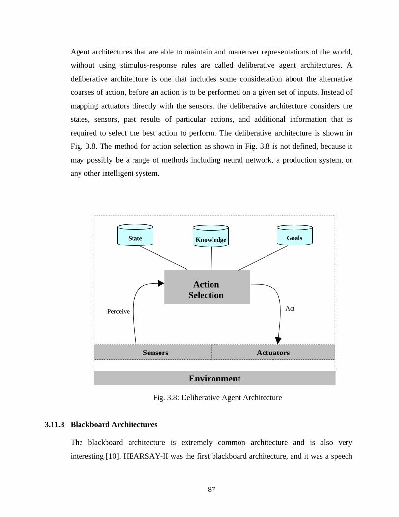
Agent architectures that are able to maintain and maneuver representations of the world,

without using stimulus-response rules are called deliberative agent architectures. A

deliberative architecture is one that includes some consideration about the alternative

courses of action, before an action is to be performed on a given set of inputs. Instead of

mapping actuators directly with the sensors, the deliberative architecture considers the

states, sensors, past results of particular actions, and additional information that is

required to select the best action to perform. The deliberative architecture is shown in

Fig. 3.8. The method for action selection as shown in Fig. 3.8 is not defined, because it

may possibly be a range of methods including neural network, a production system, or

any other intelligent system.

Fig. 3.8: Deliberative Agent Architecture

3.11.3 Blackboard Architectures

The blackboard architecture is extremely common architecture and is also very

interesting [10]. HEARSAY-II was the first blackboard architecture, and it was a speech

87

Environment

Sensors Actuators

Action Selection

KnowledgeState Goals

Perceive Act

Sensors Actuators

understanding system. This architecture works around a global work area called the

blackboard. The blackboard is a universal work area for a number of agents that operate

cooperatively to solve a particular problem. Therefore, the blackboard consists of

information about the environment, but the cooperative agents produce intermediate work

results. Fig. 3.9 shows an example blackboard architecture that could be applied to an

agent system. In this example, two different agents are employed to sample the

environment through the existing sensors (i.e., the sensor agent), and also through the

actuators available in the system.

The blackboard keeps the current state of the environment that is regularly updated by the

sensor, and when an action has to be performed, the action agent interprets this action

into control of the actuators. One or more reasoning agents actually provide the control of

the agent system. These agents work jointly to accomplish the goals, which would also be

enclosed in the blackboard. In this example, the first reasoning agent might employ the

goal definition behaviors, while the second reasoning agent may possibly implement the

planning portion.

As the blackboard is a universal work area, coordination between the agents should be

provided so that the agents do not step over one another. That is why, agents are

programmed based on their need, e.g., agents can examine the blackboard, and when

information is added, they can ask for the ability to operate. The scheduler can then

decide which agents wish to work on the blackboard, and then activate them accordingly.

The blackboard agent architecture is easily implemented on a multi-threading system.

With every agent can become one or more system threads. That is why; the blackboard

architecture is extremely common for the implementation of agent and non-agent

systems.

88

Environment

Sensors Actuators

BlackboardPerceive Act

SensorAgent

Reasoning Agent

Reasoning Agent

ActionAgent

Sensors Actuators

Fig. 3.9: Blackboard Agent Architecture

3.11.4 Belief-Desire-Intention (BDI) Architecture

BDI (Belief-Desire-Intention) agent architectures are deliberative architectures that

follow the theory of human reasoning and having planning abilities as defined by

Michael Bratman [123]. When agents are modeled within BDI architecture, they

internally indicate their beliefs, desires, and intentions and used practical reasoning to

make a decision about action selection. For an agent, belief means the view of the world

(i.e., what the agent beliefs about the state of the environment), desires are the goals

(what the agent wants to achieve) of an agent, and Intentions indicate that the Beliefs and

Desires are used by agents in order to select one or more actions, to meet the desired

goals (see Fig. 3.10). Therefore, the BDI architecture defines the fundamental

architecture of any deliberative agent. It stores the beliefs (state of the environment),

maintains a desires (set of goals), and finally, a premeditated element that maps beliefs to

desires (to select one or more actions that change the state of the environment based on

the agent’s needs)

89

Sensors Actuators

Desires

Environment

IntentionsBeliefs

Perceptual action input output

a) Horizontal Layer b) Vertical Layer c) Vertical Layer (One pass control) (Two pass control)

Layer n

........

Layer 2

Layer 1

Layer n

........

Layer 2

Layer 1

Layer n

Layer 2

Layer 1

Fig. 3.10: BDI Agent Architecture

Many researchers have accepted that neither pure reasoning approach nor pure behavioral

approach is best suited for building agents that are able to take intelligent autonomous

actions. Intelligent autonomous actions have the capability of both reactive behavior and

reasoning. This has led to the development of variety of hybrid architectures, which try to

combine the essential elements of both deliberative and behavioral systems.

3.12 Hybrid Agents

Based on the requirement that an agent should be capable of representing both reactive

and proactive behavior, separate subsystems have been created to deal with these types of

behaviors. This architecture has different subsystems that are arranged into a set of

interacting layers. In this section, layered architectures: InteRRaP and TouringMachines

are discussed. In order to deal with both reactive and proactive behaviors, there will be at

least two layers. Therefore, different architectures are differentiated in relation to how the

control and information flows within these layers. Following are the two types of control

flow inside the layered agent architecture:

• Horizontal layering: In horizontal layering architecture, each software layer

is directly linked to the sensory input and action output. Therefore, in this case

90

Sensor Input

Action Output

Perceptual action input output

a) Horizontal Layer b) Vertical Layer c) Vertical Layer (One pass control) (Two pass control)

Layer n

........

Layer 2

Layer 1

Layer n

........

Layer 2

Layer 1

Layer n

Layer 2

Layer 1

each layer behaves like an agent by giving suggestions for particular action to

perform.

• Vertical layering: In vertically layered agent architectures, decision making

is made possible through several software layers and each layer deals with the

environment at different levels of abstraction.

The advantage of horizontal layered architecture [145] is its conceptual simplicity: if we

want an agent to display n different types of behavior, then n different layers are

implemented. However, each layer is competing with one another to produce action

suggestions; there are chances that the overall agent behavior may not be consistent. In

order to ensure consistency in the horizontally layered architectures, these types of

architectures normally contain a mediator function, which decides about the particular

control layer to be active at any time. Such a central control can sometimes become very

problematic, and the designers must consider all potential interactions between layers.

Fig. 3.11: Horizontal and Vertical Layering

91

Sensor Input

Action Output

Perceptual action input output

a) Horizontal Layer b) Vertical Layer c) Vertical Layer (One pass control) (Two pass control)

Layer n

........

Layer 2

Layer 1

Layer n

........

Layer 2

Layer 1

Layer n

Layer 2

Layer 1

action output

Perceptual input

Perceptual input

action output

If there are n layers in the agent architecture, and each layer can suggest up to m possible

actions, it means there are mn possible interactions to be considered. This is undoubtedly

very difficult from a design point of view. The presence of mediator function in the agent

architecture also introduces a bottleneck into the decision making process.

These problems are partially solved in vertical layered architectures. The vertically

layered architectures can be subdivided into one-pass and two-pass architectures. In one-

pass architectures, control passes serially through each layer, until it reaches the final

layer where the action output is generated. In two-pass architectures, information first

flows up the top-most layer of the architecture (the first pass) and then control flows back

down.

Fig. 3.12: Horizontal Layered Architecture (Touring Machines)

In one-pass and two-pass vertically layered agent architectures, the complexity of inter-

layers interactions is reduced: as there are n - 1 interfaces present between n layers, and if

each layer is able to suggest m actions, then at the most m2(n - 1) interactions can be

92

Cooperative Planning

Local Planipcation

Behavior

Sensor Input

Action Output

Modling Layer

Planning Layer

Reactive Layer

Control Subsystem

Action SubsystemPerception Subsystem

considered between the layers. It is much simpler than the horizontally layered

architecture. But, this simplicity in the vertical architectures comes at the cost of decrease

in flexibility i.e. in order to take a decision the control has to pas through different layers.

This architecture is also not fault tolerant; the failure of process at any layer is most like

to have serious effects on the performance of an agent.

3.13 Conclusion

In this chapter, a comprehensive survey of the existing channel allocation schemes has

been done. The chapter also discussed various agent architectures that are used to solve

different real time problems. The next chapter presents an Optimized Blocking Dropping

Load Balancing (OBDBLB) algorithm.

Chapter 4

Optimized Blocking Dropping Load Balancing

(OBDLB) Algorithm

4.1Introduction

This chapter builds a specialized model based on hybrid agents and proposes an

Optimized Blocking Dropping Load Balancing (OBDLB) algorithm for efficient channel

allocation.

4.2INTERRAP: Vertical Layered Architecture

INTERRAP is a technique to model resource-bounded interacting agents by associating

reactivity with deliberation and cooperation capabilities [123]. INTERRAP is based on a

BDI architecture, i.e., the informational, motivational, and deliberative state of an agent

[9], which is explained through beliefs, goals, a rather generalized version of plans, and

93

Cooperative Planning

Local Planipcation

Behavior