chapter 3 design & analysis of experiments 1 7e 2009 montgomerynoordin/s/aqe ch03 rev.pdf ·...
TRANSCRIPT
Chapter 3 Design & Analysis of Experiments 7E 2009 Montgomery
1
What If There Are More Than T F L l ?Two Factor Levels?
• The t-test does not directly applyy pp y• There are lots of practical situations where there are
either more than two levels of interest, or there are l f t f i lt i t tseveral factors of simultaneous interest
• The analysis of variance (ANOVA) is the appropriate analysis “engine” for these types of experimentsanalysis engine for these types of experiments
• The ANOVA was developed by Fisher in the early 1920s, and initially applied to agricultural experiments
• Used extensively today for industrial experiments
Chapter 3 Design & Analysis of Experiments 7E 2009 Montgomery
2
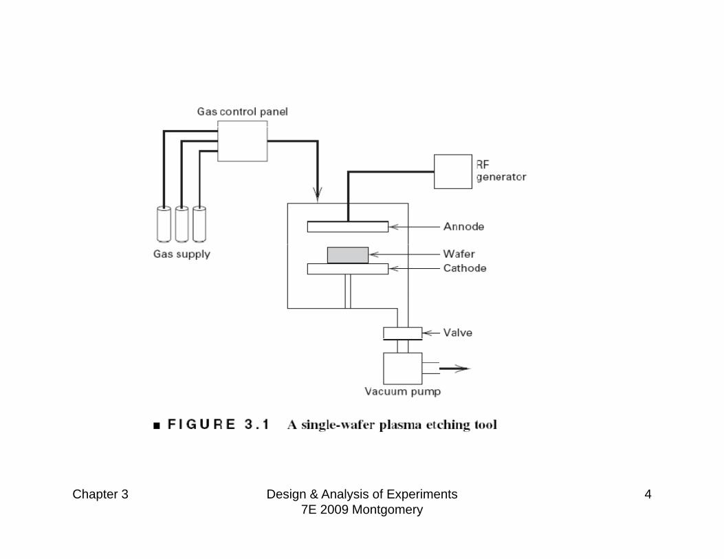
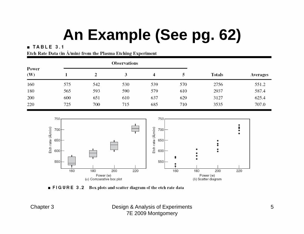
An Example (See pg. 61)An Example (See pg. 61)• An engineer is interested in investigating the relationship
bet een the RF po er setting and the etch rate for this tool Thebetween the RF power setting and the etch rate for this tool. The objective of an experiment like this is to model the relationship between etch rate and RF power, and to specify the power setting that will give a desired target etch rate.setting that will give a desired target etch rate.
• The response variable is etch rate.• She is interested in a particular gas (C2F6) and gap (0.80 cm),
and wants to test four levels of RF power: 160W 180W 200Wand wants to test four levels of RF power: 160W, 180W, 200W, and 220W. She decided to test five wafers at each level of RF power.
• The experimenter chooses 4 levels of RF power 160W, 180W, p p , ,200W, and 220W
• The experiment is replicated 5 times – runs made in random order
Chapter 3 Design & Analysis of Experiments 7E 2009 Montgomery
3
Chapter 3 Design & Analysis of Experiments 7E 2009 Montgomery
4
An Example (See pg. 62)
Chapter 3 Design & Analysis of Experiments 7E 2009 Montgomery
5
• Does changing the power change the mean etch rate?
• Is there an optimum level for power?• We would like to have an objectiveWe would like to have an objective
way to answer these questions• The t test really doesn’t apply here• The t-test really doesn t apply here –
more than two factor levels
Chapter 3 Design & Analysis of Experiments 7E 2009 Montgomery
6

The Analysis of Variance (Sec. 3.2, pg. 62)
• In general, there will be a levels of the factor, or a treatments, and n replicates of the experiment, run in random order…a completely randomized design (CRD)
• N = an total runsW id th fi d ff t th d ff t• We consider the fixed effects case…the random effects case will be discussed later
• Objective is to test hypotheses about the equality of the a treatment means
Chapter 3 Design & Analysis of Experiments 7E 2009 Montgomery
7
treatment means

The Analysis of VarianceTh “ l i f i ” f• The name “analysis of variance” stems from a partitioning of the total variability in the response variable into components that areresponse variable into components that are consistent with a model for the experiment
• The basic single-factor ANOVA model is• The basic single-factor ANOVA model is
1,2,...,i a
, , ,,
1,2,...,ij i ijyj n
2
an overall mean, treatment effect,
experimental error (0 )i ith
NID
Chapter 3 Design & Analysis of Experiments 7E 2009 Montgomery
8
experimental error, (0, )ij NID

Models for the DataModels for the Data
There are several ways to write a modelThere are several ways to write a model for the data:
is called the effects modelij i ijy
Let , then is called the means model
i i
y
is called the means model
Regression models can also be employedij i ijy
Chapter 3 Design & Analysis of Experiments 7E 2009 Montgomery
9

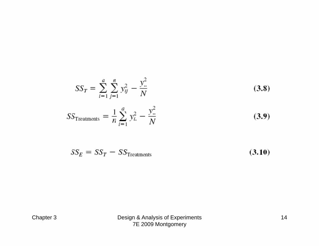
The Analysis of Variancey• Total variability is measured by the total
sum of squares:2
..1 1
( )a n
T iji j
SS y y
• The basic ANOVA partitioning is:a n a n
2 2.. . .. .
1 1 1 1( ) [( ) ( )]
a n a n
ij i ij ii j i j
a a n
y y y y y y
2 2. .. .
1 1 1( ) ( )i ij i
i i j
T T t t E
n y y y y
SS SS SS
Chapter 3 Design & Analysis of Experiments 7E 2009 Montgomery
10
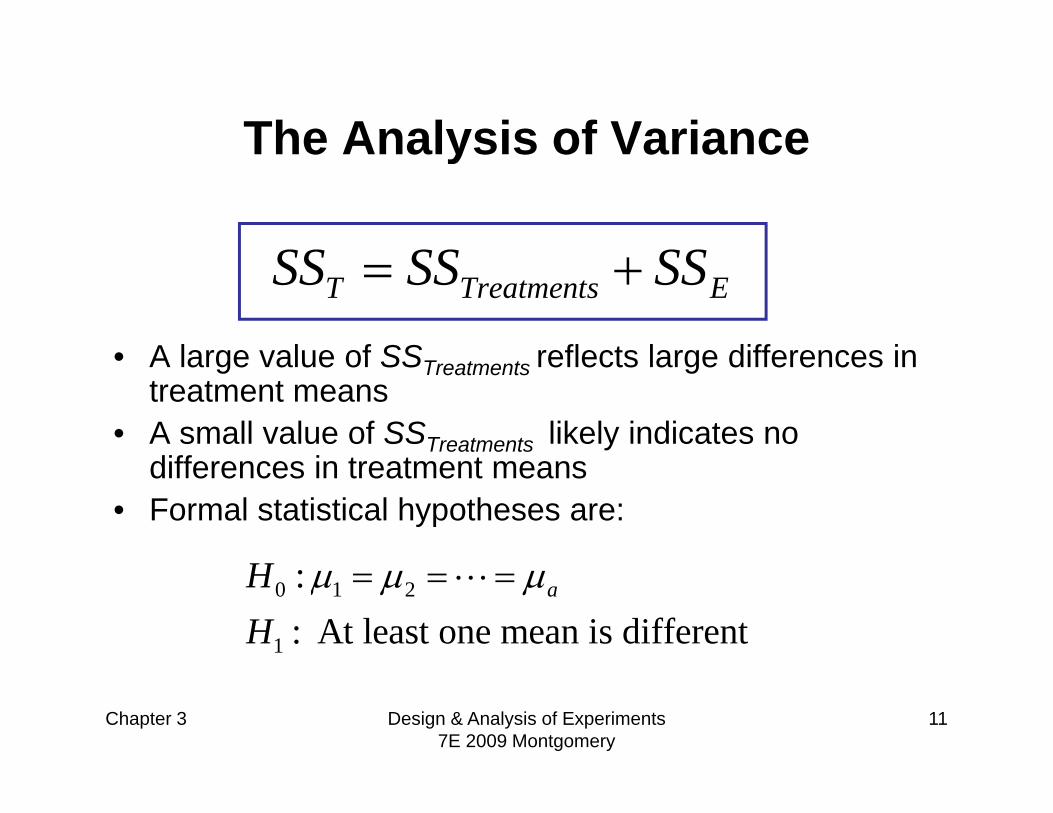
T Treatments ESS SS SS
The Analysis of VarianceThe Analysis of Variance
SS SS SS• A large value of SS reflects large differences in
T Treatments ESS SS SS
• A large value of SSTreatments reflects large differences in treatment means
• A small value of SSTreatments likely indicates no diff i t t tdifferences in treatment means
• Formal statistical hypotheses are:
0 1 2
1
:: At least one mean is different
aHH
Chapter 3 Design & Analysis of Experiments 7E 2009 Montgomery
11

The Analysis of Variance• While sums of squares cannot be directly compared
to test the hypothesis of equal means, mean squares can be compared.
• A mean square is a sum of squares divided by its degrees of freedom:
df df df1 1 ( 1)
Total Treatments Errordf df dfan a a n
,1 ( 1)
Treatments ETreatments E
SS SSMS MSa a n
• If the treatment means are equal, the treatment and error mean squares will be (theoretically) equal.
• If treatment means differ, the treatment mean square
Chapter 3 Design & Analysis of Experiments 7E 2009 Montgomery
12
If treatment means differ, the treatment mean square will be larger than the error mean square.

The Analysis of Variance is Summarized in a Table
• Computing…see text, pp 69Th f di t ib ti f F i th F di t ib ti• The reference distribution for F0 is the Fa-1, a(n-1) distribution
• Reject the null hypothesis (equal treatment means) if
0 1 ( 1)a a nF F
Chapter 3 Design & Analysis of Experiments 7E 2009 Montgomery
13
0 , 1, ( 1)a a n
Chapter 3 Design & Analysis of Experiments 7E 2009 Montgomery
14
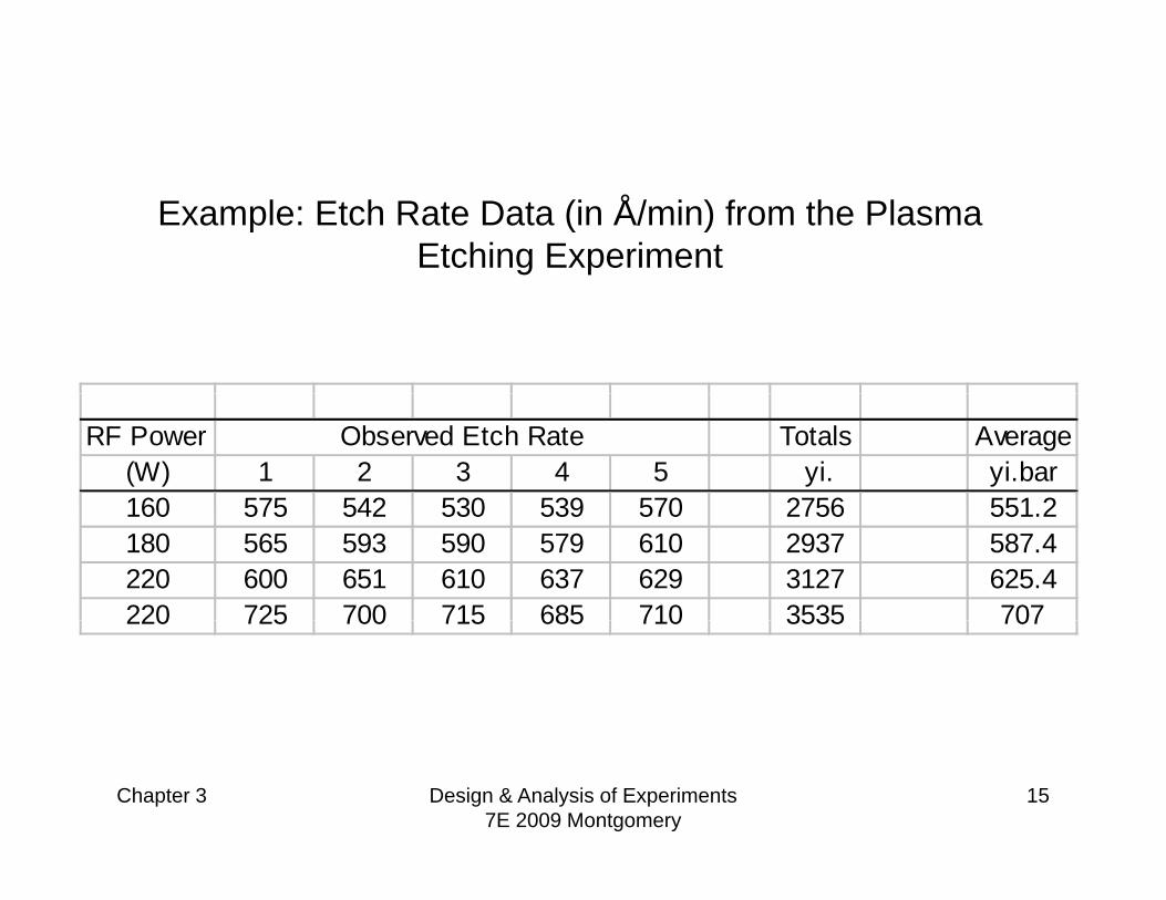
Example: Etch Rate Data (in Å/min) from the Plasma Etching Experiment
RF Power Totals Average(W) 1 2 3 4 5 yi. yi.bar160 575 542 530 539 570 2756 551 2
Observed Etch Rate
160 575 542 530 539 570 2756 551.2180 565 593 590 579 610 2937 587.4220 600 651 610 637 629 3127 625.4220 725 700 715 685 710 3535 707220 725 700 715 685 710 3535 707
Chapter 3 Design & Analysis of Experiments 7E 2009 Montgomery
15
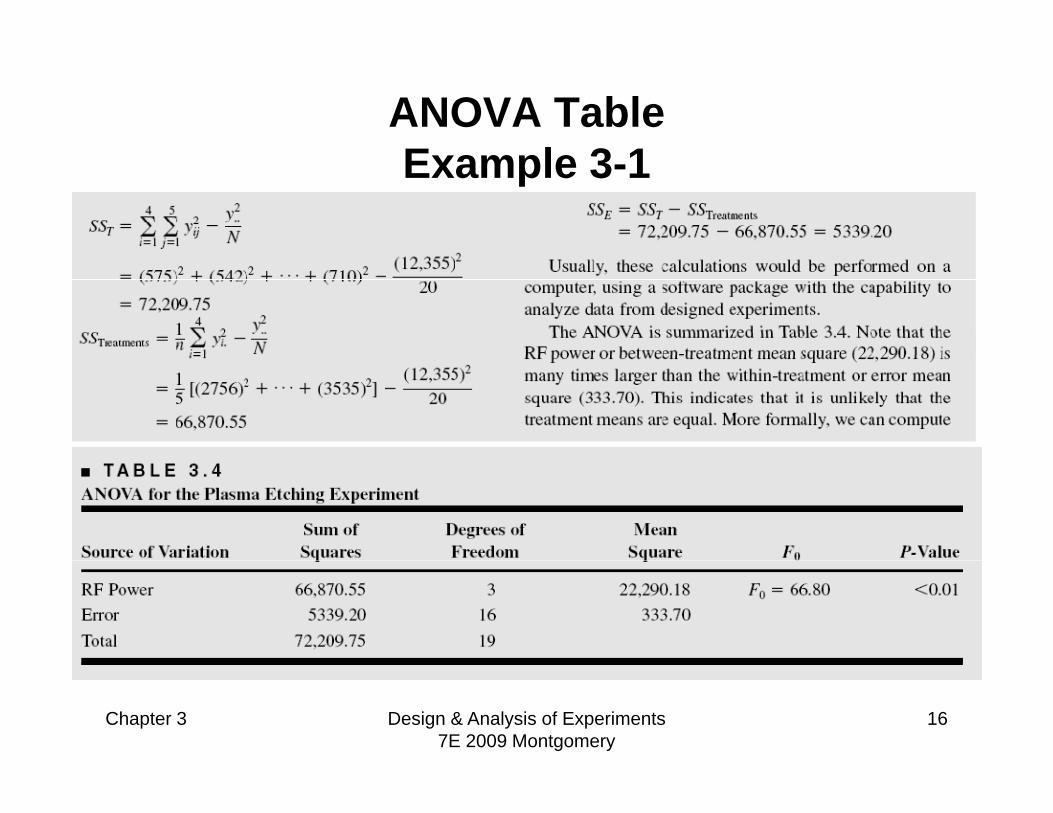
ANOVA TableE l 3 1Example 3-1
Chapter 3 Design & Analysis of Experiments 7E 2009 Montgomery
16
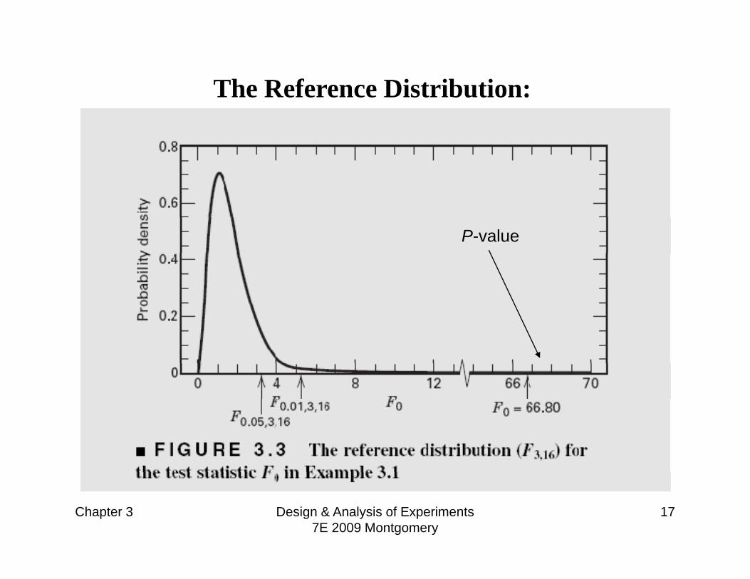
The Reference Distribution:
P-value
Chapter 3 Design & Analysis of Experiments 7E 2009 Montgomery
17

ANOVA calculations may be made simpler by coding the observation. Observation may be coded by subtracting each data by 600. We get:
Based on the data above the sum of squares may beBased on the data above, the sum of squares may be computed in the usual manner. The sum of squares are similar to that calculated previously. Therefore subtracting a constant from the original data does not change the sum
DOX 6E Montgomery 18
a constant from the original data does not change the sum of squares.
Model Adequacy Checking in the ANOVAT t f S ti 3 4 75Text reference, Section 3.4, pg. 75
Ch ki ti i i t t• Checking assumptions is important• Normality• Constant variance• IndependenceIndependence• Have we fit the right model?
L t ill t lk b t h t t d if• Later we will talk about what to do if some of these assumptions are i l t d
Chapter 3 Design & Analysis of Experiments 7E 2009 Montgomery
19
violated
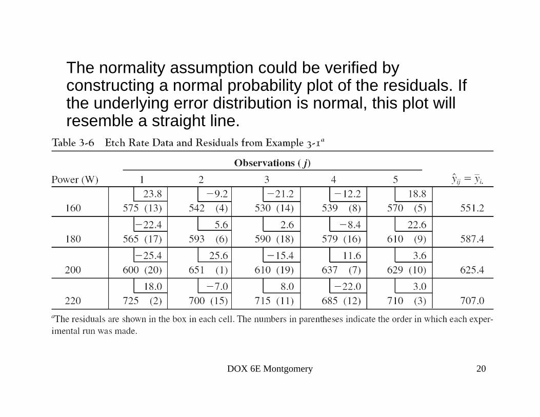
The normality assumption could be verified by constructing a normal probability plot of the residuals. If the underlying error distribution is normal, this plot will resemble a straight line.
DOX 6E Montgomery 20

Model Adequacy Checking in the ANOVA
• Examination of residuals (see text, Sec. 3 4 75)3-4, pg. 75)
ˆij ij ije y y
• Computer software
.ij iy y
Computer software generates the residuals
• Residual plots are very usefuluseful
• Normal probability plotof residuals
Chapter 3 Design & Analysis of Experiments 7E 2009 Montgomery
21

Plot of residuals in time sequence• Plotting the residuals in timePlotting the residuals in time
order of data collection is helpful in detecting correlation b t th id lbetween the residuals.
• A tendency to have runs of positive and negative residuals p gindicates positive correlation. This would imply that the independence assumption onindependence assumption on the errors has been violated.
• Important to prevent the problem and proper randomization of the experiment is an important
DOX 6E Montgomery 22
experiment is an important step in obtaining independence.
• Skill of the experimenter may improve as the experiment progresses or the process may drift. This p p g p ywill often result in a change in the error variance over time depicted by more spread at one end than at the otherother.
DOX 6E Montgomery 23
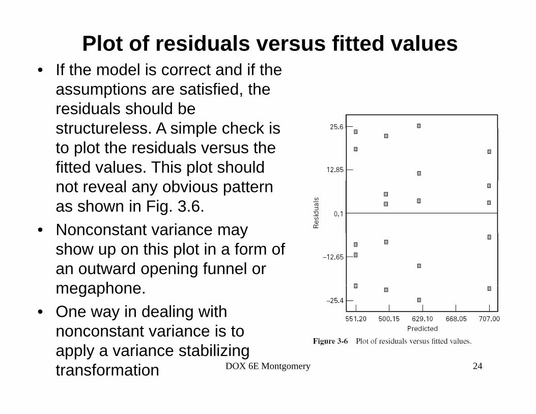
Plot of residuals versus fitted values• If the model is correct and if the
assumptions are satisfied, the residuals should be structureless A simple check isstructureless. A simple check is to plot the residuals versus the fitted values. This plot should
t l b i ttnot reveal any obvious pattern as shown in Fig. 3.6.
• Nonconstant variance mayNonconstant variance may show up on this plot in a form of an outward opening funnel or megaphonemegaphone.
• One way in dealing with nonconstant variance is to
DOX 6E Montgomery 24apply a variance stabilizing transformation
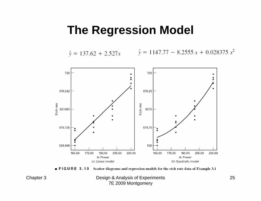
The Regression Model
Chapter 3 Design & Analysis of Experiments 7E 2009 Montgomery
25
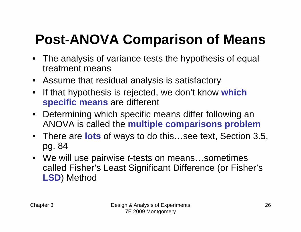
Post-ANOVA Comparison of MeansPost ANOVA Comparison of Means• The analysis of variance tests the hypothesis of equal
treatment means• Assume that residual analysis is satisfactory• If that hypothesis is rejected, we don’t know which
specific means are differentspecific means are different • Determining which specific means differ following an
ANOVA is called the multiple comparisons problem• There are lots of ways to do this…see text, Section 3.5,
pg. 84• We will use pairwise t-tests on means sometimesWe will use pairwise t tests on means…sometimes
called Fisher’s Least Significant Difference (or Fisher’s LSD) Method
Chapter 3 Design & Analysis of Experiments 7E 2009 Montgomery
26

Design-Expert Output
Chapter 3 Design & Analysis of Experiments 7E 2009 Montgomery
27

Graphical Comparison of MeansT t 88Text, pg. 88
Chapter 3 Design & Analysis of Experiments 7E 2009 Montgomery
28

ANOVA calculations are usually done via tcomputer
• Text exhibits sample calculations fromText exhibits sample calculations from three very popular software packages, Design-Expert JMP and MinitabDesign Expert, JMP and Minitab
• See pages 98-100T t di f th• Text discusses some of the summary statistics provided by these packages
Chapter 3 Design & Analysis of Experiments 7E 2009 Montgomery
29

Figure 3.12 (p. 99) Design-Expert computer output f E l 3 1for Example 3-1.
9261.0757220955.668702 Model
SSSS
R
• R2 is loosely interpreted as the proportion of the variability in the data
75.72209TotalSS
variability in the data explained by the ANOVA model. Values closer to 1 is desirable.
• Adjusted R2 reflects the number of factors in the model and useful for evaluating the impact ofevaluating the impact of increasing or decreasing the number of model terms.
• Others – see text pg. 98
DOX 6E Montgomery 30
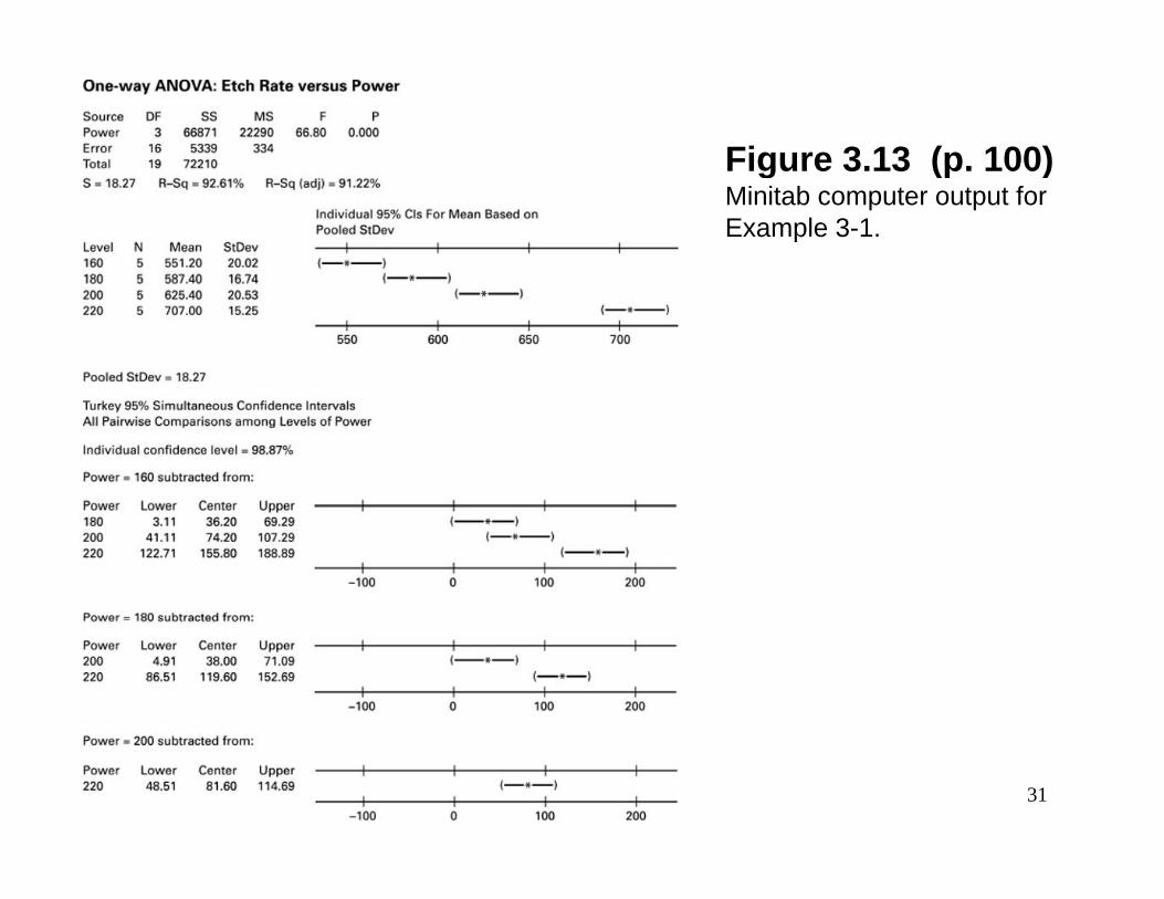
Figure 3.13 (p. 100)Figure 3.13 (p. 100)Minitab computer output for Example 3-1.
DOX 6E Montgomery 31
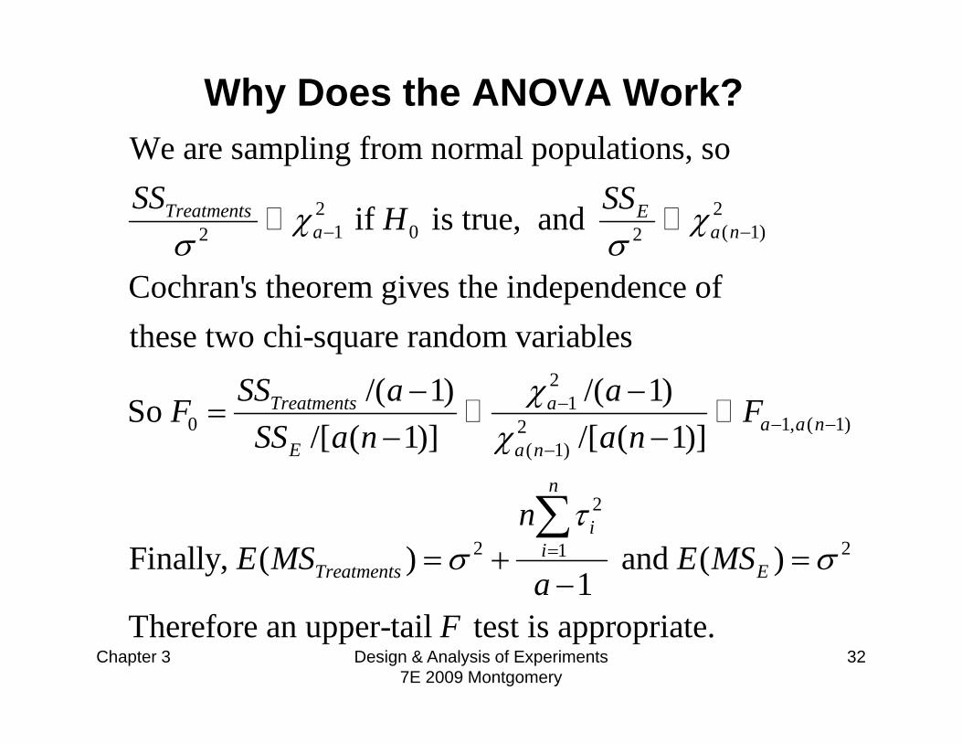
Why Does the ANOVA Work?W li f l l i
2 21 0 ( 1)2 2
We are sampling from normal populations, so
if is true, and Treatments Ea a n
SS SSH 1 0 ( 1)2 2,
Cochran's theorem gives the independence of h hi d i bl
a a n
0
these two chi-square random variables/(So TreatmentsSSF
21
1 ( 1)1) /( 1)aa a F
0So F 1, ( 1)2( 1)
2
/[ ( 1)] /[ ( 1)] a a nE a n
n
FSS a n a n
n
2 21Finally, ( ) and ( )
1
ii
Treatments E
nE MS E MS
a
Chapter 3 Design & Analysis of Experiments 7E 2009 Montgomery
32Therefore an upper-tail test is appropriate.F

Sample Size DeterminationText, Section 3.7, pg. 101
• FAQ in designed experimentsFAQ in designed experiments• Answer depends on lots of things; including
what type of experiment is being yp p gcontemplated, how it will be conducted, resources, and desired sensitivityS iti it f t th diff i• Sensitivity refers to the difference in meansthat the experimenter wishes to detect
• Generally increasing the number ofGenerally, increasing the number of replications increases the sensitivity or it makes it easier to detect small differences in
Chapter 3 Design & Analysis of Experiments 7E 2009 Montgomery
33
means
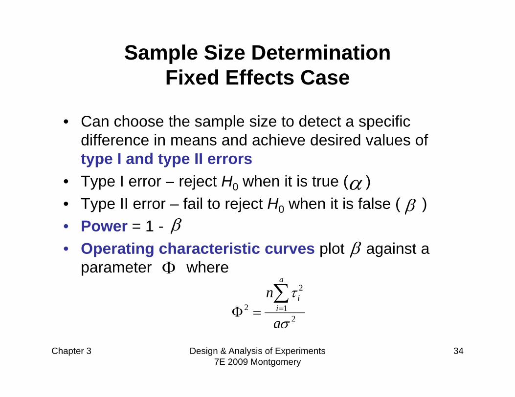
Sample Size DeterminationFi d Eff t CFixed Effects Case
• Can choose the sample size to detect a specificCan choose the sample size to detect a specific difference in means and achieve desired values of type I and type II errors
• Type I error – reject H0 when it is true ( )• Type II error – fail to reject H0 when it is false ( )
Power = 1
• Power = 1 -• Operating characteristic curves plot against a
parameter where
p2
2 12
a
ii
n
a
Chapter 3 Design & Analysis of Experiments 7E 2009 Montgomery
34
a
Sample Size DeterminationFi d Eff t C f OC CFixed Effects Case---use of OC Curves
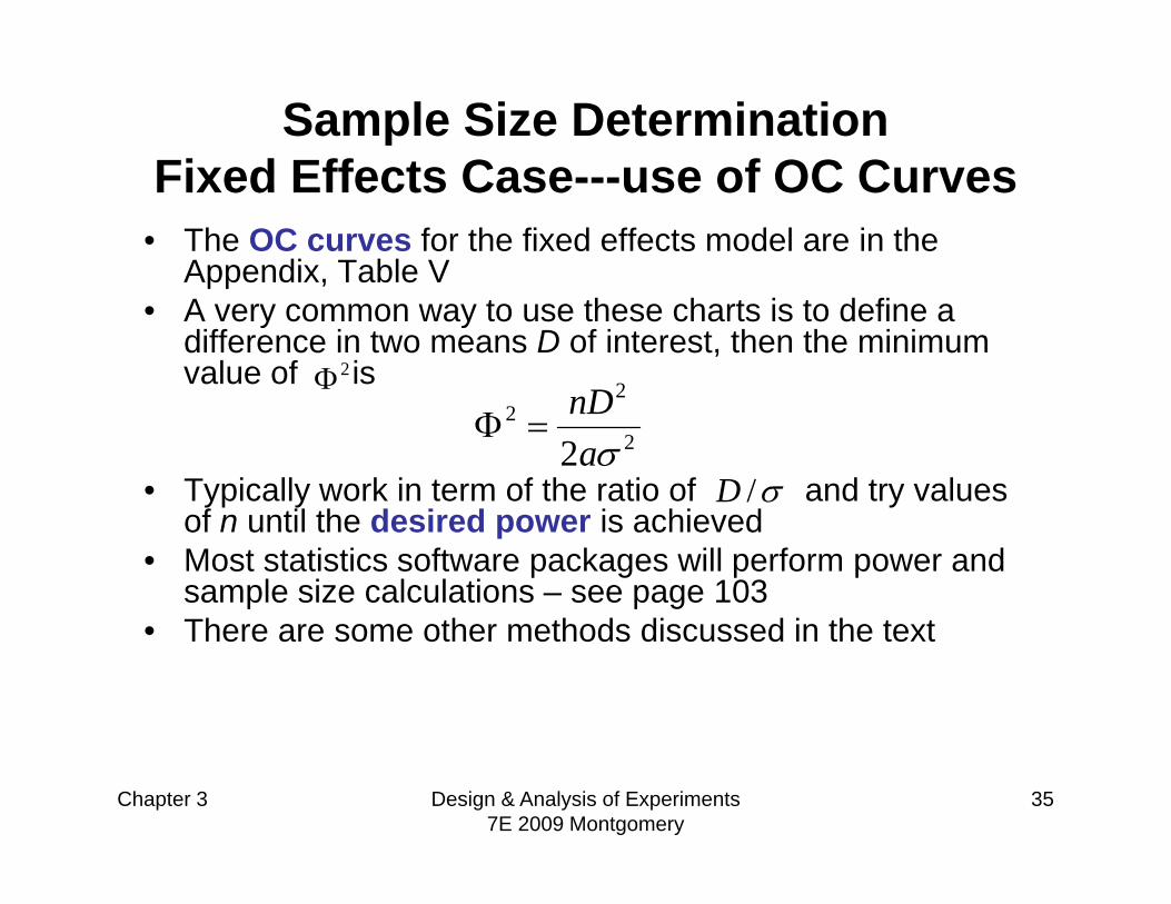
• The OC curves for the fixed effects model are in the Appendix, Table VAppendix, Table V
• A very common way to use these charts is to define a difference in two means D of interest, then the minimum value of is2 2D
• Typically work in term of the ratio of and try values f il h d i d i hi d
22
22nDa
/D of n until the desired power is achieved
• Most statistics software packages will perform power and sample size calculations – see page 103Th th th d di d i th t t• There are some other methods discussed in the text
Chapter 3 Design & Analysis of Experiments 7E 2009 Montgomery
35

Power and sample size calculations from Minitab (Page 103)
Chapter 3 Design & Analysis of Experiments 7E 2009 Montgomery
36

Chapter 3 Design & Analysis of Experiments 7E 2009 Montgomery
37
Chapter 3 Design & Analysis of Experiments 7E 2009 Montgomery
38
Chapter 3 Design & Analysis of Experiments 7E 2009 Montgomery
39
Chapter 3 Design & Analysis of Experiments 7E 2009 Montgomery
40
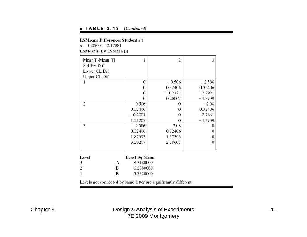
Chapter 3 Design & Analysis of Experiments 7E 2009 Montgomery
41
Question to be attemptedQuestion to be attempted
• Chapter 3Chapter 3No. 3.1, 3.3, 3.6, 3.9(N 3 7 3 8 3 11 3 5)(No. 3.7, 3.8, 3.11, 3.5)
DOX 6E Montgomery 42