59

CHAPTER 3

FINITE ELEMENT MODELING OF

TIBIA BONE AND IMPLANT

3.1 INTRODUCTION

3.1.1 Construction of CAD based bio modeling

Although non-invasive modalities, such as CT, Micro CT, MRI and

Optical Microscopy can be used to produce accurate 3D tissue descriptions,

the voxel-based anatomical imaging representation cannot be effectively used

in many biomechanical engineering studies. For example, 3D surface

extraction requires either a large amount of computational power or extreme

sophistication in data organisation and handling 3D volumetric model and on

the other hand, while producing a realistic 3D anatomical appearance, does

not contain geometric topological relation. Although they are capable of

describing the anatomical morphology and are applicable to RP through a

converted STL format, neither of them is capable of performing anatomical

structural design, modeling-based anatomical tissue bio mechanical analysis

and simulation. In general, activities in anatomical modeling design, analysis

and simulation need to be carried out in a vector-based modeling

environment, such as using CAD system and CAD-based solid modeling,

which is usually represented as ‘Boundary Representation’ (B-REP) and

mathematically described as Non-Uniform Rational B-Spline (NURBS)

functions. Unfortunately, the direct conversion of the medical imaging data

60

CT images

2D segmentation

MedCAD interface

Polyline fit on the contour of the model

Output polylines as IGES curves

3D region growing

Fit a B-Spline surface on the polyline on each slice

CAD model

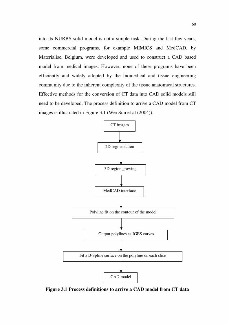
into its NURBS solid model is not a simple task. During the last few years,

some commercial programs, for example MIMICS and MedCAD, by

Materialise, Belgium, were developed and used to construct a CAD based

model from medical images. However, none of these programs have been

efficiently and widely adopted by the biomedical and tissue engineering

community due to the inherent complexity of the tissue anatomical structures.

Effective methods for the conversion of CT data into CAD solid models still

need to be developed. The process definition to arrive a CAD model from CT

images is illustrated in Figure 3.1 (Wei Sun et al (2004)).

Figure 3.1 Process definitions to arrive a CAD model from CT data

61

3.2 COMPUTED TOMOGRAPHY (CT)

In the early period the methods used to derive bone geometry and

mechanical properties were inaccurate and sometimes highly invasive and

destructive. CT images provide accurate information about bone geometry.

The Radiographic Density (RD) reported in the CT images can be related to

the mechanical properties of bone. Moreover, CT scanning is a mildly

invasive routine diagnostic method which permits the modeling of human

bones in vivo. CT scans are far more detailed than ordinary X-rays. The

information from the 2D computer images can be reconstructed to produce

3D images by some modern CT scanners. They can be used to produce virtual

images that show what a surgeon would see during an operation. Digital

Imaging and Communications in Medicine (DICOM) is a standard for

handling, storing, printing and transmitting information in medical imaging.

Therefore CT or MRI is not only a complementary technique for diagnosis

but also an important aid as its emerging technique is vital for professional

awareness, producing a virtual model and creating a physical model is

becoming popular. A thorough understanding on the basics of those

techniques is necessary for surgeons to make a model for diagnosis and

treatment planning, according to their need, rather than to depend on the

technicians. In this work, the 2D images in the DICOM format are obtained

from Siemens make CT machine to perform modeling, simulation and

analysis of patient-specific implant for RM. The input data of the modeling

process represented by tomography slices in DICOM format belongs to 23

year old adult male with a Body Weight (BW) of 80 Kg which contains 1173

tomography slices as shown in the Figures 3.2 and 3.3. The dimension of each

file is 512 x 512 pixels with the distance of 1mm between them.

62

Figure 3.2 2D slice images from CT in DICOM format

Figure 3.3 3D stacking image data in DICOM format

63

3.3 MIMICS

Materialise’s Interactive Medical Image Control Systems

(MIMICS), is a user-friendly 3D medical image processing and editing

software. It translates scanner data into full 3D CAD models, FE meshes or

RP data within minutes and allows simulating surgical procedures. This

software package is used to convert the CT data into a series of contours to

simulate outer cortical and intramedullary bone marrow surfaces by

segmentation and 3D rendering objects.

3.3.1 Import modules

MIMICS imports 2D stacked images such as CT, MRI or

Microscopy data in a wide variety of formats, far beyond DICOM. The import

software provides direct access to images written on proprietary optical disks

and tapes, converts them into the Materialise image format and preserves all

necessary information for further processing. The DICOM format is a

standard in the Medical Imaging world and most recent scanners are DICOM

compliant. MIMICS can import DICOM images that are compressed with the

JPEG algorithm.

3.3.2 Visualisation

MIMICS displays the image data in several ways, each providing

unique information. MIMICS include several visualisation functions such as

contrast enhancement, panning, zooming and rotating of the 3D view.

MIMICS divide the screen into four views as shown in the Figure 3.4,

a) The original axial view

b) The coronal view (made up by the resliced data)

c) The sagittal view (made up by the resliced data) and

d) The 3D view

64

Axial view (a)

Coronal view (b)

Sagittal view (c)

3D view (d)

Figure 3.4 Various views of CT images are loaded and registered in

MIMICS

3.3.3 Segmentation

In MIMICS, segmentation masks are used to highlight Regions Of

Interest (ROI). MIMICS enable one to define and process images with up to

30 coloured segmentation masks. To create and modify these masks, the

following functions are used:

Thresholding

Thresholding is the first action performed to create a segmentation

mask. ROI by defining a range of gray values to select a specific area as

shown in the Figure 3.5. For extracting the cortical and trabacular tibial bone

features accurately, threshold value is adjusted from 226 to 1956 Hounsfield

Units (HU) in the MIMICS which corresponds to the bone density interval.

The accuracy of the model is comprised by 3 times smoothing.

65

Region Growing

Region growing eliminates noise and separate structures that have

failed to connect. Then region growing is used to separate the ROI from the

selected object. In this work, the 3D model of the left side Tibia bone is

selected as a ROI to generate the patient-specific fracture implant. To check

the result, 3D model has to be evaluated.

Editing (Draw, Erase, Local Threshold)

Manual editing functions make it possible to draw, erase or restore

parts of images with a local threshold value. With the multiple slice edit tool,

the changes can be made on one slice to other slices. This tool greatly reduces

the amount of manual work needed to eliminate artifacts and separate

structures.

Figure 3.5 ROI is identified as appropriate differentiating colour mask

66

Dynamic Region Growing

Dynamic region growing segments an object based on the

connectivity of gray values in a certain gray value range. It allows for easy

segmentation of tendons and nerves in CT images, as well as providing an

overall useful tool for working with MRI images.

3.3.4 3D rendering and 3D information

MIMICS provide a flexible interface for quickly calculating a 3D

model of the ROI. Information about height, width, volume, surface, etc. is

available for every 3D model. During 3D reconstruction processes, each pixel

of the formed mask is converted into voxel as shown in the Figure 3.6. The

value of each voxel depends on the scanning distance between slices.

MIMICS can display the 3D model in any of the windows with visualisation

functions that include real-time rotation, pan, zoom and transparency.

Figure 3.6 3D voxel based reconstructed tibia bone model

67

Advanced rendering

The ability to apply advanced rendering with OpenGL hardware

acceleration offers high-quality rendering for optimal display of the 3D

objects. By using the clipping functions, it is possible to view inside a 3D

object or see how an STL is located on the images and much more.

3.3.5 MedCAD interface

The MedCAD interface, normally a standard module of medical

image processing software, is intended to bridge the gap between medical

imaging and CAD design software. The MedCAD interface can export data

from the imaging system to the CAD platform and vice versa through either

IGES (International Graphics Exchange Standard), STEP (Standard for

Exchange of Product) or STL format. The interface provides for fitting of

primitives such as cylinders, planes, spheres etc with the (imaging) 2D

segmentation slices. It also provides the limited ability to model a freeform

surface (such as B-spline surfaces). The limitation of using MedCAD

interface is the incapability to capture detail and complex tissue anatomical

features, particularly for features with complex geometry.

Then Med CAD module in the MIMICS is used to export the 3D

model data from imaging system to the CAD system as IGES file format as

shown in the Figure 3.7. For each section polylines have been generated, so

that 1677 polylines are obtained from tomography slices. This can be

exported for further CAD analysis.

68

Bone marrow

Cortical bone

Figure 3.7 CAD model construction using MedCAD interface

3.4 CAD MODELING OF TIBIA BONE USING CATIA

3.4.1 Introduction

CATIA (Computer Aided Three dimensional Interactive

Application) is a multi-platform CAD/CAM/CAE commercial software suite

developed by the French company Dassault Systems and marketed worldwide

by IBM.

3.4.2 Modeling of tibia bone

The 3D tibia bone model generated in polylines exported from

MIMICS software as IGES format has been imported into CAD software

CATIA, which is used as a reference model to model the anatomy specific

bone model and implant for any fracture as shown in the Figure 3.8. CATIA

is used to process the data in order to create NURBS surfaces, which are

easily handled by Finite Element software (Wei Sun and Pallavi Lal (2002)).

69

Figure 3.8 IGES file imported into CATIA

Hence the splines are created as shown in the Figure 3.9 over the

polylines to obtain the surface model of the bone which is having inner and

outer boundary. Modeling these boundaries is used to assign the material

properties of the regions of bone at the time of Finite Element Modeling

(FEM). Because of the complicated geometrical configuration of the 3D model,

the model cannot be directly exported in CAD software. Thus the solid model

of tibia is transformed to a detailed 3D model, which contains IGES surfaces.

Figure 3.9 Splines created on the polylines

70

The accuracy of the model is depending upon the CT slice

thickness. If number of slice increases or thickness of the slices decreases,

then the accuracy of the model will be increased. Some of the data loss in the

CT images can be rectified using the editing tool of the software by adding

the pixels on the sections. It would help to design the precise patient-specific

implant model. After editing the data such as blending, joining, smoothing,

filling gaps, etc. on the splines, the curves as shown in the Figure 3.10 are

wrapped as closed surfaces. The final model is obtained by inserting a

surface, which is tangent to all polylines from top to bottom.

Figure 3.10 Surface models of cortical and bone marrow regions of tibia

bone

3.5 PRE-PROCESSING USING HYPERMESH

Analysis or evaluation of the models is done by finite disordering to

elements for detailed analysis. This pre-processing is carried out as follow.

3.5.1 Introduction

Altair HyperMesh is a high-performance finite element pre-

processor that provides a highly interactive and visual environment to analyse

product design performance. With the broadest set of direct interfaces to

commercial CAD and CAE systems, HyperMesh provides a proven,

consistent analysis platform for the entire enterprise. With a focus on

engineering productivity, HyperMesh is the user-preferred environment for:

Bone marrow Cortical bone Distal end

Proximal end

Shaft

71

HyperMesh presents users with an advanced suite of easy-to-

use tools to build and edit CAE models.

For 2D and 3D model creation, users have access to a variety

of mesh-generation capabilities, as well as HyperMesh’s

powerful auto meshing module.

3.5.2 Meshing

Surface Meshing

The surface meshing module in HyperMesh contains a robust

engine for mesh generation that provides users with unparalleled flexibility

and functionality. This includes the ability to interactively adjust a variety of

mesh parameters, optimize a mesh based on a set of user defined quality

criteria and create a mesh using a wide range of advanced techniques.

Solid Meshing

Using solid geometry, HyperMesh can utilise both standard and

advanced procedure to connect, separate or split solid models for tetra-

meshing or hexa-meshing. Partitioning these models is fast and easy when

combined with HyperMesh's powerful visualisation features for solids. This

allows users to spend less time preparing geometries for solid meshing. The

solid-meshing module allows users to quickly generate high quality meshes

for multiple volumes.

Mesh Morphing

Hyper Morph is powerful solution for interactively and parametrically

changing the shape of a FEM. Its unique approach enables rapid shape variations

on the finite element mesh without sacrificing mesh quality. During the

morphing process, Hyper Morph also allows the creation of shape variables,

which can be used for subsequent design optimization studies.

72

Batch Meshing

Using Altair Batch Mesher is the fastest way to automatically

generate high-quality finite element meshes for large assemblies. By

minimising manual meshing tasks, this auto-meshing technology provides

more time for value-added engineering simulation activities. Batch Mesher

provides user-specified control over meshing criteria and geometry clean-up

parameters as well as the ability to output to customise model file formats.

3.5.3 CAD Interoperability

HyperMesh provides direct readers for industry-leading CAD data

formats for generating FEM. Moreover, HyperMesh has robust tools to clean

up (mend) imported geometry containing surfaces with gaps, overlaps and

misalignments that prevent high-quality mesh generation. By eliminating

misalignments and holes, and suppressing the boundaries between adjacent

surfaces users can mesh across larger, more logical regions of the model

while improving overall meshing speed and quality. Boundary conditions can

be applied to these surfaces for future mapping to underlying element data.

3.5.4 Geometry interfacing and clean up of tibia bone

The CAD model of tibia bone is developed and modeled through

CATIA IGES file; this is imported into HyperMesh software, to clean up

imported geometry containing surfaces with gaps, overlaps and

misalignments that prevent high-quality mesh generation. By eliminating

misalignments and holes, and suppressing the boundaries between adjacent

surfaces, the overall meshing speed and quality is improved. The influence of

mesh density on the model accuracy was investigated using different FE

meshes (tetrahedral elements) of the tibia bone with increasing numbers of

elements and nodes to determine convergence of the solution. The FE model

73

with 68,740 elements and 15,365 nodes was accepted for this study. The

Figure 3.11 shows that the model is meshed to 3 mm element size and the

quality is checked. Element type and Boundary conditions are applied to these

surfaces for future mapping to underlying element data. FE model is

developed for the entire length of the Tibial bone measuring 415 mm in

length.

Figure 3.11 Preprocessing the model

The model is divided into three regions named as thick shaft region

as cortical bone, bone marrow inside the cortical and spongy region in

proximal and distal end of the bone as trabacular. During normal walking

stance phase at full extension, the peak load acting on the human tibial region

is 3 times body weight of the person (Cinzia Zannoni et al (1998) and

Harrington (1976)). A loading condition of 2400N (BW-80 kg) is applied on

the proximal region which is split into 60 % (1470 N) of weight in the medial

region and 40 % (930 N) in the lateral region of the model. The load is

approximately distributed in the middle of the medial and lateral regions as

shown in the Figure 3.12. The linear elastic, orthotropic and heterogeneous

material property is assigned for the cortical region (Taylor et al (2002) and

Cortical bone

Bone marrow

bone

74

Ashman et al (1989)). Also, the linear elastic, isotropic and homogeneous

material property is assigned for both trabacular and bone marrow (Rho et al

(1995)) bone regions as shown in the Table 3.1. Poisson’s ratio ( ) for all the

three regions is considered as 0.3. The bulk modulus (G) for cortical bone was

calculated using the formula given in the Equation 3.1,

3E = 2G (1+ ) (3.1)

where E- young’s modulus, G- Bulk modulus and -poison’s ratio. The

degrees of freedom of the nodes in the distal end of the bone were totally

constrained. Then the model is imported into ANSYS 10.0 software to

perform the FEA of intact (without fracture) bone by assigning real constant

and element type. Pre Conjugate Solver (PCS) is used to solve the problem

and the mechanical properties such as displacement, stress and strain are

identified. As a person stands, the tibia does not collapse, but every particle

within it deforms to a minute extent and strain develops. As the bone deforms,

there are forces of molecular cohesion holding it together and resisting the

applied load. If the load is too great and exceeds these intermolecular forces,

the equilibrium is destroyed and bone breaks.

Table 3.1 Material property assigned for bone regions

No DescriptionMaterial

Property

Young’s

modulus (GPa)

Poison’s

ratio

1 Cortical bone

Linearly elastic,

orthotropic,

heterogeneous

Ex : 12.50

Ey : 14.00

Ez : 21.75

xy : 0.376

yz : 0.235

zx : 0.222

2 Bone marrow 0.1 0.3

3 Trabacular bone

Linearly elastic,

isotropic,

homogeneous17.5 0.3

75

Figure 3.12 Loading and boundary conditions

3.5.5 Modeling of lateral impact condition

After completion of modeling and reconstruction, the tibia model is

imported into ANSYS LSDYNA software to provide the original geometry

information. The lateral impact environment is simulated using 30 kg weight

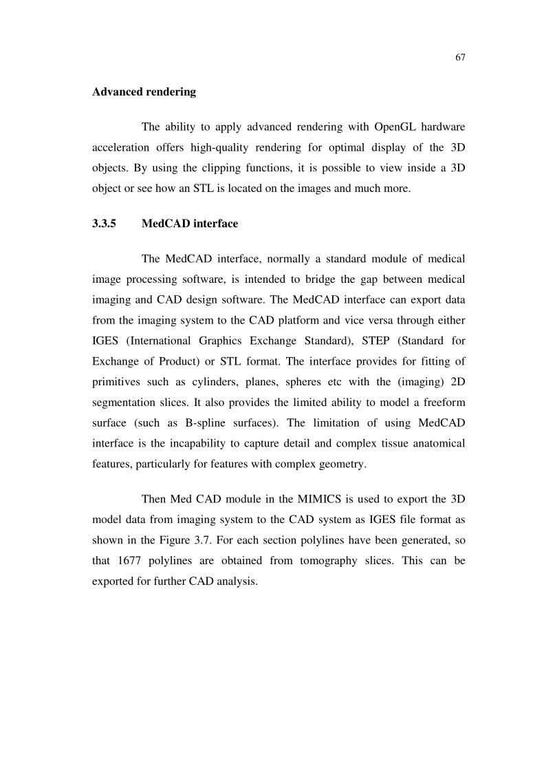
impact bar, made up of Stainless Steel of size 350 x 75 x 45 mm as shown in

the Figure 3.13. The dynamic analysis is carried out for an impact velocity of

4 m/sec. To produce impact loading, the force is applied for the time span of

4 µs. In this study, joints near proximal (knee) and distal end (foot) are not

considered. Also the ligament and muscle forces are not included, since these

are negligible compared to the impact force. Impact bar’s deformations or

stress distributions are also not considered. But the impactor mass and impact

velocity are included, since it is necessary to find the energy absorbed by the

bone before the fracture. As a contact problem, the bone is defined as the

Proximal end

Constrained distal end

Lateral load (930 N)

Medial load (1470 N)

Bone

76

target surface and impact bar as the contact surface. Stepped load is used and

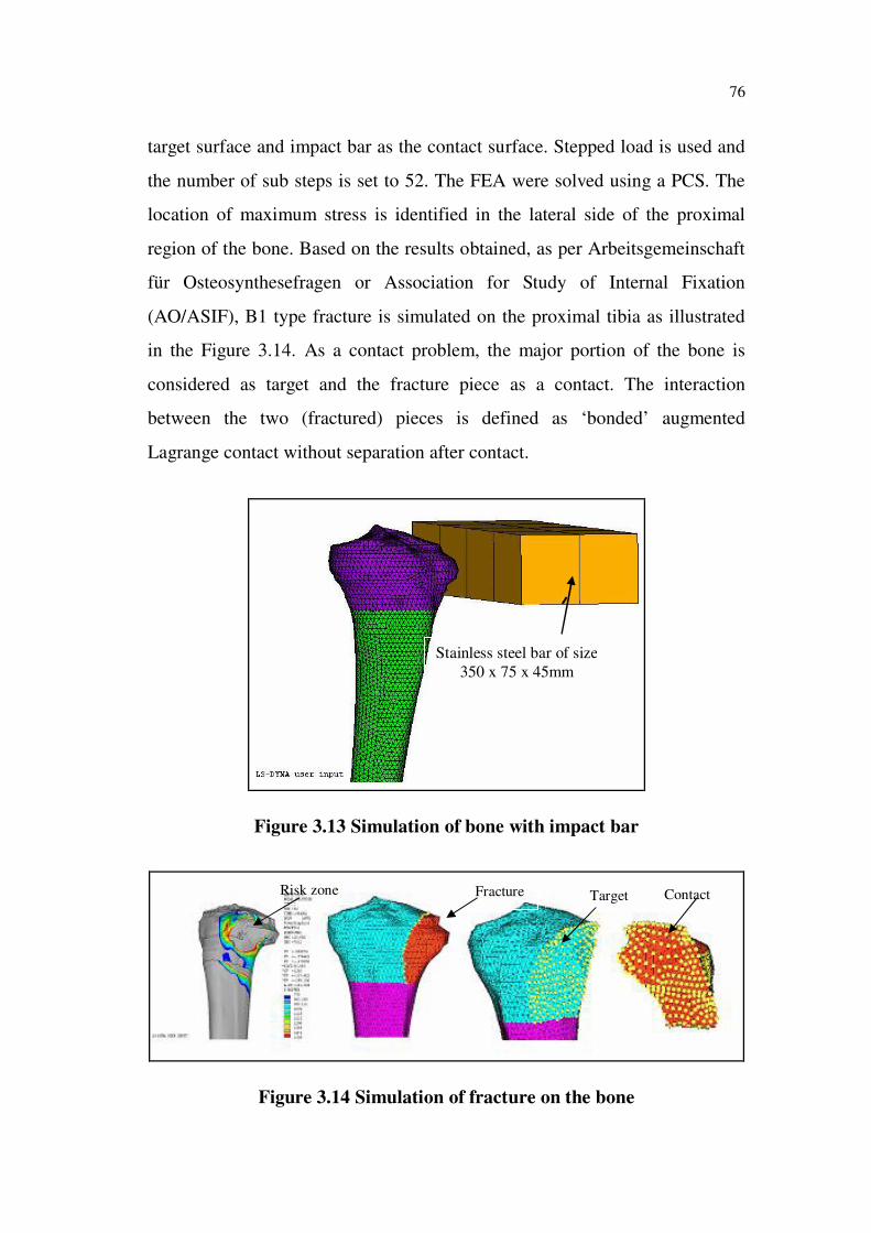
the number of sub steps is set to 52. The FEA were solved using a PCS. The

location of maximum stress is identified in the lateral side of the proximal

region of the bone. Based on the results obtained, as per Arbeitsgemeinschaft

für Osteosynthesefragen or Association for Study of Internal Fixation

(AO/ASIF), B1 type fracture is simulated on the proximal tibia as illustrated

in the Figure 3.14. As a contact problem, the major portion of the bone is

considered as target and the fracture piece as a contact. The interaction

between the two (fractured) pieces is defined as ‘bonded’ augmented

Lagrange contact without separation after contact.

Figure 3.13 Simulation of bone with impact bar

Figure 3.14 Simulation of fracture on the bone

Stainless steel bar of size

350 x 75 x 45mm

ContactTargetFractureRisk zone

77

3.6 MODELING OF PRE-FABRICATED AND PATIENT-

SPECIFIC IMPLANTS

3.6.1 Introduction

The implants are often anatomically shaped or contoured designs

versus basic geometric shapes and produced as a family in a range of sizes

that can be selected at surgery to match the patient requirement. The pre-bent

implant results in more compressive contact across the fracture site without

gapping. Gap may result in micro movements with subsequent bone

resorption and loss of fixation. An implant must be sufficiently long and

strong and should be fixed with an adequate number of screws to provide

rigid fixation for successful treatment of a fracture (Baris Simsek et al

(2006)).

Patient-specific implants are necessary for those situations when an

off-the shelf standard size is not suitable. These are usually complex cases

involving trauma or disease resulting in bone deformity or loss (Ola Harryson

et al (2007)). A patient-specific implant is produced on a prescription basis

and is unique for each patient. Most commonly used implants for fracture

fixation are often limited by their biological and mechanical constraints (Ming

- Yih Lee et al (2002)). The bio mechanical considerations while designing

the implants, improves the longevity of the implant and provides stability to

the bone-implant construct. Sharing of load by implants creates favourable

mechanical conditions for healing. In evaluating the long term success of an

implant, the reliability and the stability of the implant and bone-implant

interface plays a great role (Ola Harryson et al (2007)). Analysis of force

transfer at bone-implant interface is an essential step in the overall analysis of

loading, which determines the success or failure of an implant.

78

3.6.2 Modeling of pre-fabricated implant

The commercially available pre-fabricated implant in the market,

manufactured by M/s Greens Surgicals Private Limited, Vadodara, India as

per AO/ASIF recommendations is being used as a reference for modeling

both the pre-fabricated and patient-specific implant. Some of the fracture

fixation for proximal side of the tibia bone is shown in the Figure 3.15.

Among these, T-Buttress plate is considered for modeling, analysis and

fabrication of patient-specific implant.

Figure 3.15 Implants for proximal left tibia fracture

A portable non-contact FARO Photon Laser Scanner measurement

system (Divija Technologies, Tamil Nadu, India) to accurately capture 3D

data is used to reverse engineer the T-Buttress plate. The system rotates 360°

and measures everything within its line of sight up to 120 m away. With a

scan rate of 976,000 points per seconds and an accuracy of up to ± 2 mm it

can be used in a wide range of industries. The surface model details obtained

from the scan is imported as IGES format to translate into CAD software for

modeling and other purposes as illustrated in the Figure 3.16.

T-Buttress plate

Lateral tibial head buttress plate

L-Buttress plate

Compression plate

79

Figure 3.16 Surface model translated into CATIA

3.6.3 Modeling of patient-specific implant

The CAD model of the bone developed from the CT image is used

to develop the patient-specific implant for proximal tibial fracture. In order to

promote better bone ingrowths and uniform stress distribution, it is decided to

construct the patient-specific implant by extracting the surface features of the

bone. The inner surface of the implant should be parametric as well as it

should nearly define the external surface of the bone to get an even load

distribution and uniform thickness. The inner parametric surface i.e., bone-

implant interface is generated and it closely follows, the shape of the section

curves of the tibia bone model. This was the most challenging task.

Parameterisation feature helps to change the dimension and location of the

implant as shown in the Figure 3.17. The implant created thus is exported into

IGES format. The final model of the implant has a length of 135 mm.

80

Figure 3.17 Modeling of patient-specific implant

Figure 3.18 shows the surface model of the patient-specific implant

extracted from the bone surface. Then the thickness 2.5 mm is given to the

surface model using the contours from the implant surface, a parametric

sketch is defined on each plane. It closely follows the shape of the section

curves of the tibia model. The distance between the section curve and

parametric curve constitute the thickness of the implant as shown in the

Figure 3.19.

Figure 3.18 Surface model extracted from bone

81

Figure 3.19 2.5 mm thickness assigned over the surface of the implant

The continuity of the parametric curve has to be maintained tangent

to each other to avoid any error in the model. The final model of the implant

has a length of 135 mm and 2.5 mm thickness and was obtained using some

of the operating functions like offset, extract, fill and so on. The final model

obtained from the CAD software is used to analyse the mechanical behaviour

of bone and implant after fracture fixation at various loading and boundary

conditions. Also the CAD data is used to fabricate the patient-specific implant

directly through RM techniques.

3.7 FINITE ELEMENT ANALYSIS OF BONE WITH IMPLANT

The surface implant model developed in the CAD software is fixed

with fractured bone in the HyperMesh software. The implant material

property is assigned as linear elastic, homogeneous and isotropic. It is made

of surgical Titanium (Ti6Al4V) having an elastic modulus of 120 GPa and

poisson’s ratio of 0.3. Then the IGES format models are imported into

ANSYS software for post processing and solved to perform the analysis.

Element types, real constant, material property, thickness of implant and

82

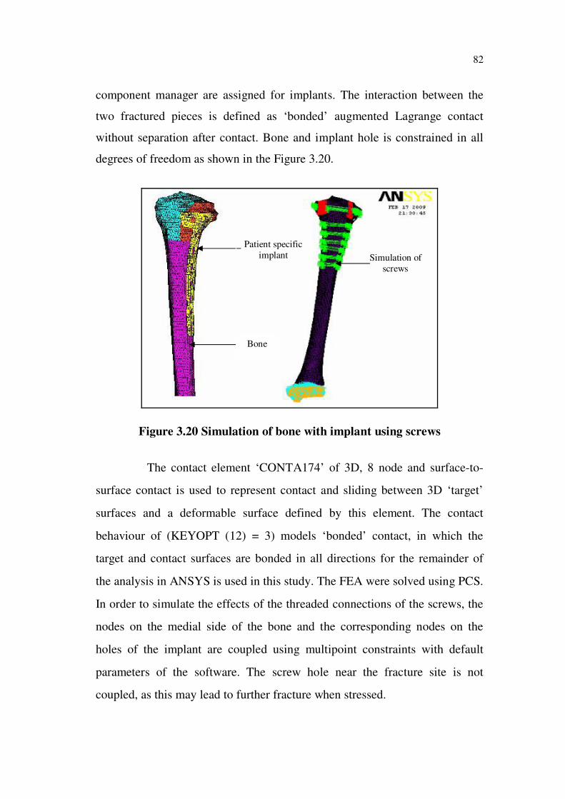
component manager are assigned for implants. The interaction between the

two fractured pieces is defined as ‘bonded’ augmented Lagrange contact

without separation after contact. Bone and implant hole is constrained in all

degrees of freedom as shown in the Figure 3.20.

Figure 3.20 Simulation of bone with implant using screws

The contact element ‘CONTA174’ of 3D, 8 node and surface-to-

surface contact is used to represent contact and sliding between 3D ‘target’

surfaces and a deformable surface defined by this element. The contact

behaviour of (KEYOPT (12) = 3) models ‘bonded’ contact, in which the

target and contact surfaces are bonded in all directions for the remainder of

the analysis in ANSYS is used in this study. The FEA were solved using PCS.

In order to simulate the effects of the threaded connections of the screws, the

nodes on the medial side of the bone and the corresponding nodes on the

holes of the implant are coupled using multipoint constraints with default

parameters of the software. The screw hole near the fracture site is not

coupled, as this may lead to further fracture when stressed.

Bone

Patient specific

implant Simulation of

screws