chapter 3 introduction to linear programmingjyee/491.06/lectures/chapter03.pdf · chapter 3...

1

1Copyright (c) 2003 Brooks/Cole, a division of Thomson Learning, Inc.

Chapter 3Introduction to Linear Programming

to accompanyIntroduction to Mathematical Programming: Operations Research, Volume 1

4th edition, by Wayne L. Winston and Munirpallam Venkataramanan

Presentation: H. Sarper


3.1 - What Is a Linear Programming Problem?

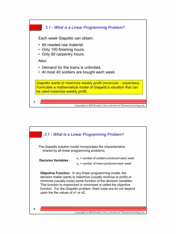
Each soldier built:• Sell for $27 and uses $19 worth of raw materials. • Increase Giapetto’s variable labor/overhead costs by $14.• Requires 2 hours of finishing labor.• Requires 1 hour of carpentry labor.

Each train built:• Sell for $21 and used $9 worth of raw materials. • Increases Giapetto’s variable labor/overhead costs by $10.• Requires 1 hour of finishing labor.• Requires 1 hour of carpentry labor.

Example

Giapetto’s, Inc., manufactures wooden soldiers and trains.

2



Each week Giapetto can obtain:

• All needed raw material. • Only 100 finishing hours.• Only 80 carpentry hours.

Also:

• Demand for the trains is unlimited.• At most 40 soldiers are bought each week.

Giapetto wants to maximize weekly profit (revenues – expenses). Formulate a mathematical model of Giapetto’s situation that can be used maximize weekly profit.



The Giapetto solution model incorporates the characteristics shared by all linear programming problems.

Decision Variablesx1 = number of soldiers produced each week

x2 = number of trains produced each week

Objective Function In any linear programming model, the decision maker wants to maximize (usually revenue or profit) or minimize (usually costs) some function of the decision variables. This function to maximized or minimized is called the objective function. For the Giapetto problem, fixed costs are do not depend upon the the values of x1 or x2.

3



Giapetto’s weekly profit can be expressed in terms of the decision variables x1 and x2:

Weekly profit =weekly revenue – weekly raw material costs – the weekly variable costs

Weekly revenue = 27x1 + 21x2

Weekly raw material costs = 10x1 + 9x2

Weekly variable costs = 14x1 + 10x2

Weekly profit =

(27x1 + 21x2) – (10x1 + 9x2) – (14x1 + 10x2 ) = 3x1 + 2x2



Thus, Giapetto’s objective is to chose x1 and x2 to maximize 3x1 + 2x2. We use the variable z to denote the objective function value of any LP. Giapetto’s objective function is:

Maximize z = 3x1 + 2x2

“Maximize” will be abbreviated by max and “minimize”by min. The coefficient of an objective function variable is called an objective function coefficient.

4



Constraints As x1 and x2 increase, Giapetto’s objective function grows larger. For Giapetto, the values of x1 and x2 are limited by the following three restrictions (often called constraints):

Constraint 1 Each week, no more than 100 hours of finishing time may be used.

Constraint 2 Each week, no more than 80 hours of carpentry time may be used.

Constraint 3 Because of limited demand, at most 40 soldiers should be produced.

These three constraints can be expressed mathematically by the following equations:

Constraint 1: 2 x1 + x2 ≤ 100

Constraint 2: x1 + x2 ≤ 80

Constraint 3: x1 ≤ 40



Sign Restrictions To complete the formulation of a linear programming problem, the following question must be answered for each decision variable: Can the decision variable only assume nonnegative values, or is the decision variable allowed to assume both positive and negative values?

If the decision variable can assume only nonnegative values, the sign restriction xi ≥ 0 is added. If the variable can assume both positive and negative values, the decision variable xi is unrestricted in sign (often abbreviated urs).

The coefficients of the constraints are often called the technological coefficients. The number on the right-hand side of the constraint is called the constraint’s right-hand side (or rhs).

5



For the Giapetto problem model, combining the sign restrictions x1 ≥ 0 and x2 ≥ 0 with the objective function and constraints yields the following optimization model:

Max z = 3x1 + 2x2 (objective function)

Subject to (s.t.)2 x1 + x2 ≤ 100 (finishing constraint)

x1 + x2 ≤ 80 (carpentry constraint)

x1 ≤ 40 (constraint on demand for soldiers)

x1 ≥ 0 (sign restriction)




Concepts of linear function and linear inequality:

Linear Function: A function f(x1, x2, …, xn of x1, x2, …, xn is a linear function if and only if for some set of constants, c1, c2, …, cn, f(x1, x2, …, xn) = c1x1 + c2x2 + … + cnxn.

For example, f(x1,x2) = 2x1 + x2 is a linear function of x1 and x2, but f(x1,x2) = (x1)

2x2 is not a linear function of x1 and x2.

For any linear function f(x1, x2, …, xn) and any number b, the inequalities inequality f(x1, x2, …, xn) ≤ b and f(x1, x2, …, xn) ≥ b are linear inequalities.

6



1. Attempt to maximize (or minimize) a linear function (called the objective function) of the decision variables.

2. The values of the decision variables must satisfy a set of constraints. Each constraint must be a linear equation or inequality.

3. A sign restriction is associated with each variable. For each variable xi, the sign restriction specifies either that xi must be nonnegative (xi ≥ 0) or that xi may be unrestricted in sign.

A linear programming problem (LP) is an optimization problem for which we do the following:



Proportionality and Additive Assumptions

The fact that the objective function for an LP must be a linear function of the decision variables has two implications:

1. The contribution of the objective function from each decision variable is proportional to the value of the decision variable. For example, the contribution to the objective function for 4 soldiers is exactly fours times the contributionof 1 soldier.

2. The contribution to the objective function for any variable is independent of the other decision variables. For example, no matter what the value of x2, the manufacture of x1 soldiers will always contribute 3x1 dollars to the objective function.

7



1. The contribution of each variable to the left-hand side of each constraint is proportional to the value of the variable. For example, it takes exactly 3 times as many finishing hours to manufacture 3 soldiers as it does 1 soldier.

2. The contribution of a variable to the left-hand side of each constraint is independent of the values of the variable. For example, no matter what the value of x1, the manufacture of x2 trains uses x2 finishing hours and x2 carpentry hours

Analogously, the fact that each LP constraint must be a linear inequality or linear equation has two implications:



Divisibility AssumptionThe divisibility assumption requires that each decision variable be

permitted to assume fractional values. For example, this assumption implies it is acceptable to produce a fractional number of trains. The Giapetto LP does not satisfy the divisibility assumption since a fractional soldier or train cannot be produced. Chapter 9 the use of integer programming methods necessary to address the solution to this problem.

The Certainty AssumptionThe certainty assumption is that each parameter (objective function

coefficients, right-hand side, and technological coefficients) are known with certainty.

8


3.1 - What Is a Linear Programming Problem?Feasible Region and Optimal Solution

x1 = 40 and x2 = 20 are in the feasible region since they satisfy all the Giapetto constraints.

On the other hand, x1 = 15, x2 = 70 is not in the feasible region because this point does not satisfy the carpentry constraint [15 + 70 is > 80].

Giapetto Constraints

2 x1 + x2 ≤ 100 (finishing constraint)


x1 ≤ 40 (demand constraint)



The feasible region of an LP is the set of all points satisfying all the LP’s constraints and sign restrictions.


3.1 - What Is a Linear Programming Problem?For a maximization problem, an optimal solution to an LP is a point

in the feasible region with the largest objective function value. Similarly, for a minimization problem, an optimal solution is a point in the feasible region with the smallest objective function value.

Most LPs have only one optimal solution. However, some LPs haveno optimal solution, and some LPs have an infinite number of solutions. Section 3.2 shows the optimal solution to the Giapetto LP is x1 = 20 and x2 = 60. This solution yields an objective function value of:

z = 3x1 + 2x2 = 3(20) + 2(60) = $180

When we say x1 = 20 and x2 = 60 is the optimal solution, we are saying that no point in the feasible region has an objective function value (profit) exceeding 180.

9


3.2 – Graphical Solution to a 2-Variable LP

Any LP with only two variables can be solved graphically. We always label the variables x1 and x2 and the coordinate axes the x1 and x2 axes.

Graphical Example:The shaded area in the

graph are the set of points satisfying the equation:

2x1 + 3x2 ≤ 6

X1

1 2 3 4

1

2

3

4

X2

-1

-1

2x1 + 3x2 ≤ 6



Finding the Feasible Solution

Since the Giapetto LP has two variables, it may be solved graphically. The feasible region is the set of all points satisfying the constraints:

Giapetto Constraints

2 x1 + x2 ≤ 100 (finishing constraint)


x1 ≤ 40 (demand constraint)



A graph of the constraints and feasible region is shown on the next slide.

10



X1

X2

10 20 40 50 60 80

2040

6080

100

f in is h in g c o n s tra in t

c a rp e n try c o n s tra in t

d e m a n d c o n s tra in t

z = 6 0

z = 1 0 0

z = 1 8 0

F e a s ib le R e g io n

G

A

B

C

D

E

F

H

From figure, we see that the set of points satisfying the Giapetto LP is bounded by the five sided polygon DGFEH. Any point on or in the interior of this polygon (the shade area) is in the feasible region.



Having identified the feasible region for the Giapetto LP, a search can begin for the optimal solution which will be the point in the feasible region with the largest z-value.

11



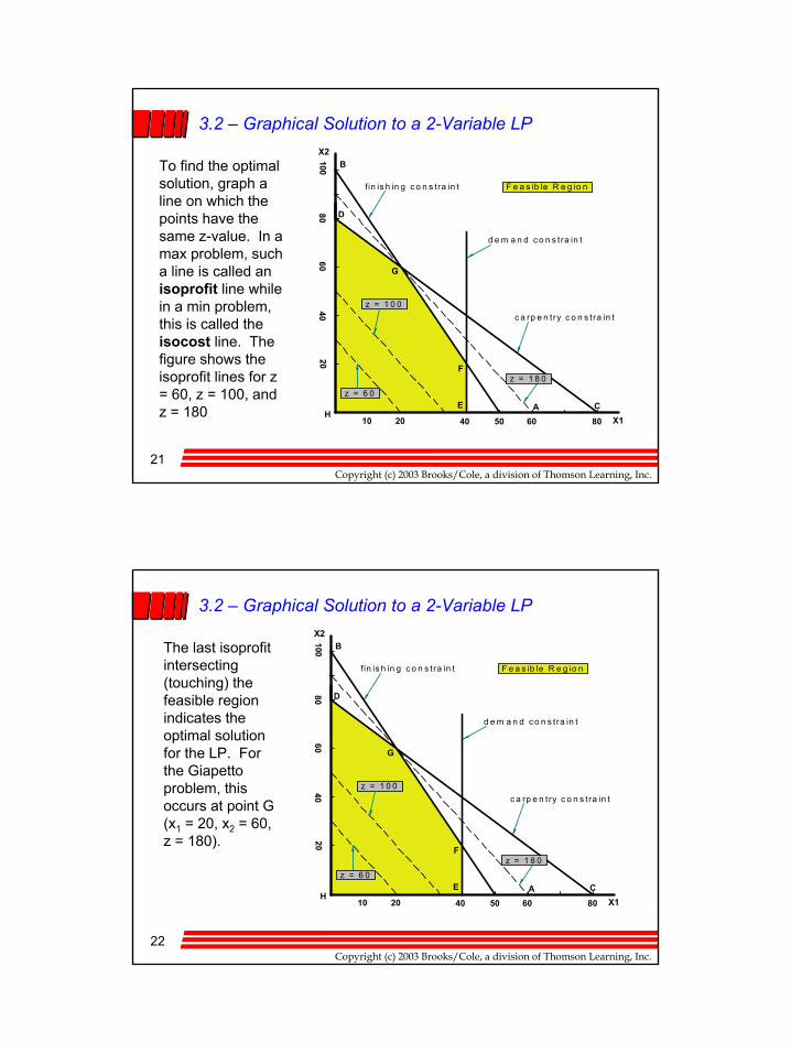
To find the optimal solution, graph a line on which the points have the same z-value. In a max problem, such a line is called an isoprofit line while in a min problem, this is called the isocost line. The figure shows the isoprofit lines for z = 60, z = 100, and z = 180

X1

X2

10 20 40 50 60 80

2040

6080

100




z = 6 0

z = 1 0 0

z = 1 8 0


G

A

B

C

D

E

F

H



The last isoprofitintersecting (touching) the feasible region indicates the optimal solution for the LP. For the Giapettoproblem, this occurs at point G (x1 = 20, x2 = 60, z = 180).

X1

X2

10 20 40 50 60 80

2040

6080

100




z = 6 0

z = 1 0 0

z = 1 8 0


G

A

B

C

D

E

F

H

12



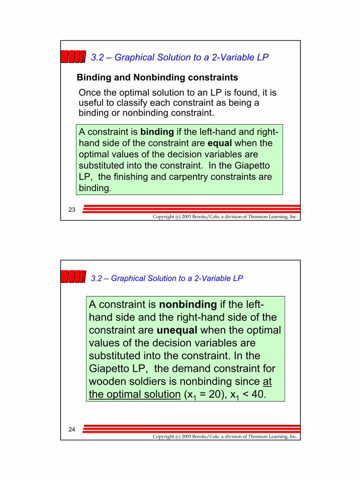
Binding and Nonbinding constraints

A constraint is binding if the left-hand and right-hand side of the constraint are equal when the optimal values of the decision variables are substituted into the constraint. In the Giapetto LP, the finishing and carpentry constraints are binding.

Once the optimal solution to an LP is found, it is useful to classify each constraint as being a binding or nonbinding constraint.



A constraint is nonbinding if the left-hand side and the right-hand side of the constraint are unequal when the optimal values of the decision variables are substituted into the constraint. In the Giapetto LP, the demand constraint for wooden soldiers is nonbinding since at the optimal solution (x1 = 20), x1 < 40.

13


3.2 – Graphical Solution to a 2-Variable LPConvex sets, Extreme Points, and LPA set of points S is a convex set if the line segment jointing any two pairs of points in S is wholly contained in S.

For any convex set S, a point p in S is an extreme point if each line segment that lines completely in S and contains the point P has P as an endpoint of the line segment.

Consider the figures (a) – (d) below:A E B

DC

A B

A B

(a) (b) (c) (d)



For example, in figures (a) and (b) below, each line segment joining points in S contains only points in S. Thus is convex for (a) and (b). In both figures (c) and (d), there are points in the line segment AB that are not in S. S in not convex for (c) and (d).

A E B

DC

A B

A B

(a) (b) (c) (d)

14



A E B

DC

A B

A B

(a) (b) (c) (d)

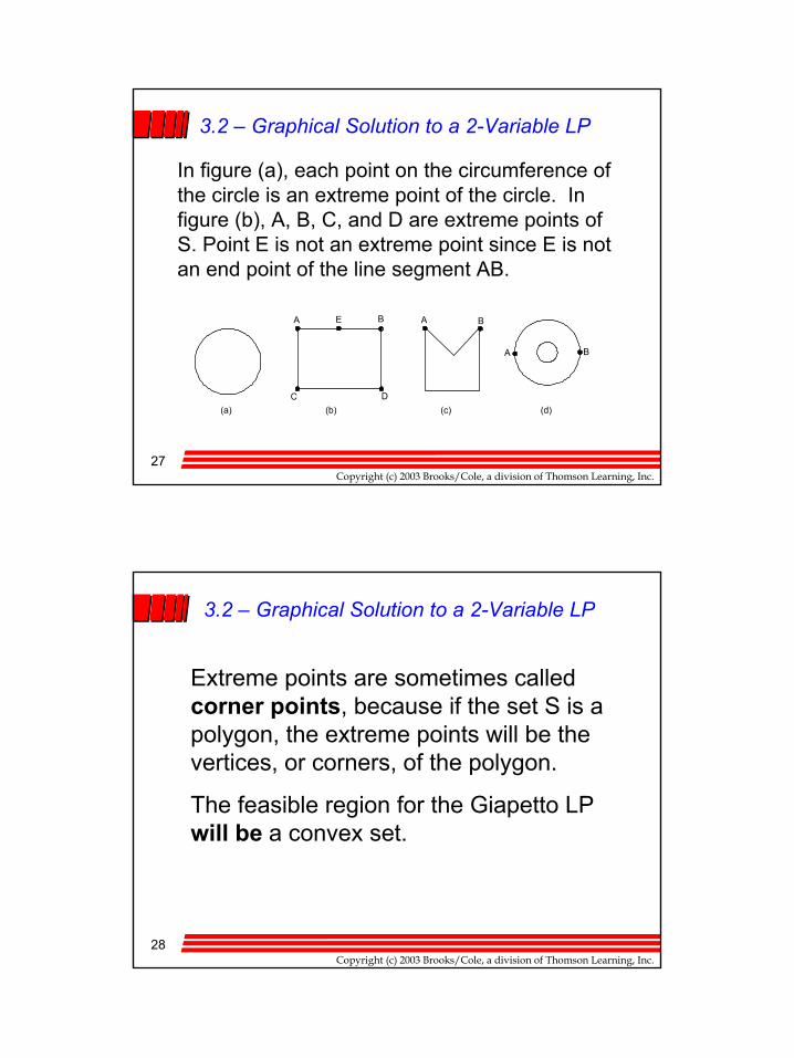
In figure (a), each point on the circumference of the circle is an extreme point of the circle. In figure (b), A, B, C, and D are extreme points of S. Point E is not an extreme point since E is not an end point of the line segment AB.



Extreme points are sometimes called corner points, because if the set S is a polygon, the extreme points will be the vertices, or corners, of the polygon.

The feasible region for the Giapetto LP will be a convex set.

15



It can be shown that:

• The feasible region for any LP will be a convex set.

• The feasible region for any LP has only a finite number of extreme points.

1.Any LP that has an optimal solution has an extreme point that is optimal.


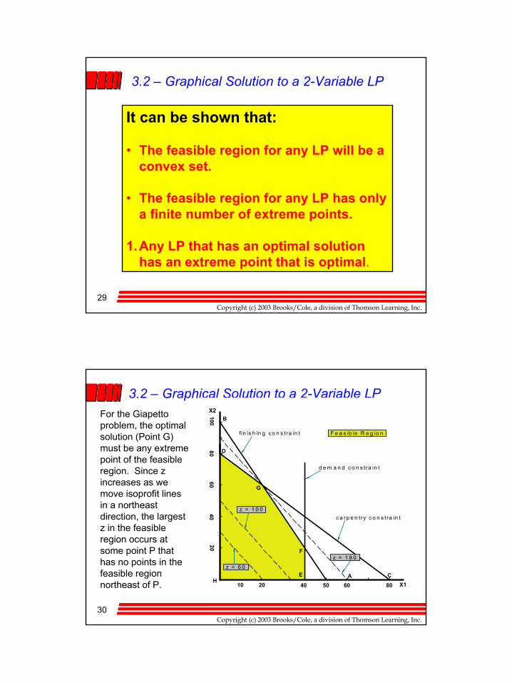
3.2 – Graphical Solution to a 2-Variable LPFor the Giapettoproblem, the optimal solution (Point G) must be any extreme point of the feasible region. Since z increases as we move isoprofit lines in a northeast direction, the largest z in the feasible region occurs at some point P that has no points in the feasible region northeast of P. X1

X2

10 20 40 50 60 80

2040

6080

100




z = 6 0

z = 1 0 0

z = 1 8 0


G

A

B

C

D

E

F

H

16


3.2 – Graphical Solution to a 2-Variable LPThis means the optimal solution must lie somewhere on the boundary of the feasible region. The LP must have an extreme point that is optimal, because for any line segment on the boundary of the feasible area, the largest z value on that line segment must be assumed at be at one endpoints of the line segment. X1

X2

10 20 40 50 60 80

2040

6080

100




z = 6 0

z = 1 0 0

z = 1 8 0


G

A

B

C

D

E

F

H



A Graphical Solution to a Minimization Problem

To reach these groups, Dorian Auto has embarked on an ambitious TV advertising campaign and has decide to purchase 1-mimute commercial spots on two type of programs: comedy shoes and football games.

Dorian Auto manufactures luxury cars and trucks. The company believes that its most likely customers are high-income women and men.

17



• Each comedy commercial is seen by 7 million high income women and 2 million high-income men.

• Each football game is seen by 2 million high-income women and 12 million high-income men.

• A 1-minute comedy ad costs $50,000 and a 1-minute football ad costs $100,000.

Dorian Auto would like for commercials to be seen by at least 28 million high-income women and 24 million high-income men.

Use LP to determine hoe Dorian Auto can meet its advertising requirements at minimum cost.



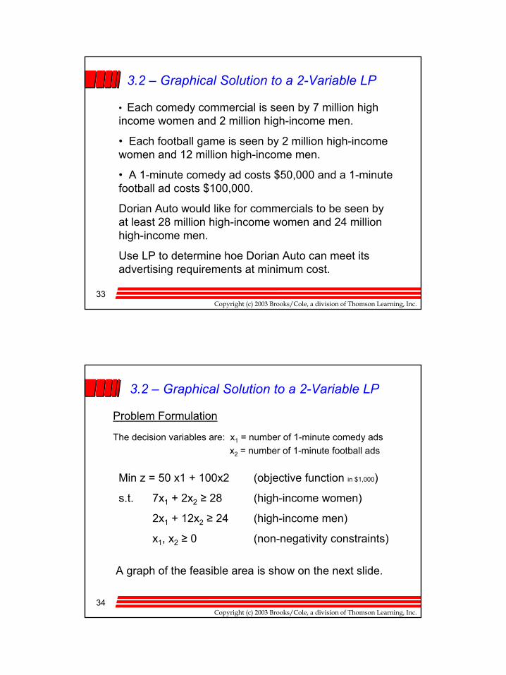
Problem Formulation

The decision variables are: x1 = number of 1-minute comedy adsx2 = number of 1-minute football ads

Min z = 50 x1 + 100x2 (objective function in $1,000)

s.t. 7x1 + 2x2 ≥ 28 (high-income women)

2x1 + 12x2 ≥ 24 (high-income men)

x1, x2 ≥ 0 (non-negativity constraints)

A graph of the feasible area is show on the next slide.

18



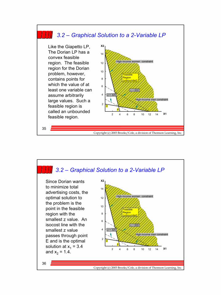
Like the Giapetto LP, The Dorian LP has a convex feasible region. The feasible region for the Dorian problem, however, contains points for which the value of at least one variable can assume arbitrarily large values. Such a feasible region is called an unbounded feasible region.

X1

X2

2

4

6

8

10

12

14

2 4 6 8 10 12 14

z = 600

z = 320

A CD

E

B

Feasible Region (unbounded)

High-income women constraint

High-income men constraint



X1

X2

2

4

6

8

10

12

14

2 4 6 8 10 12 14

z = 600

z = 320

A CD

E

B




Since Dorian wants to minimize total advertising costs, the optimal solution to the problem is the point in the feasible region with the smallest z value. An isocost line with the smallest z value passes through point E and is the optimal solution at x1 = 3.4 and x2 = 1.4.

19



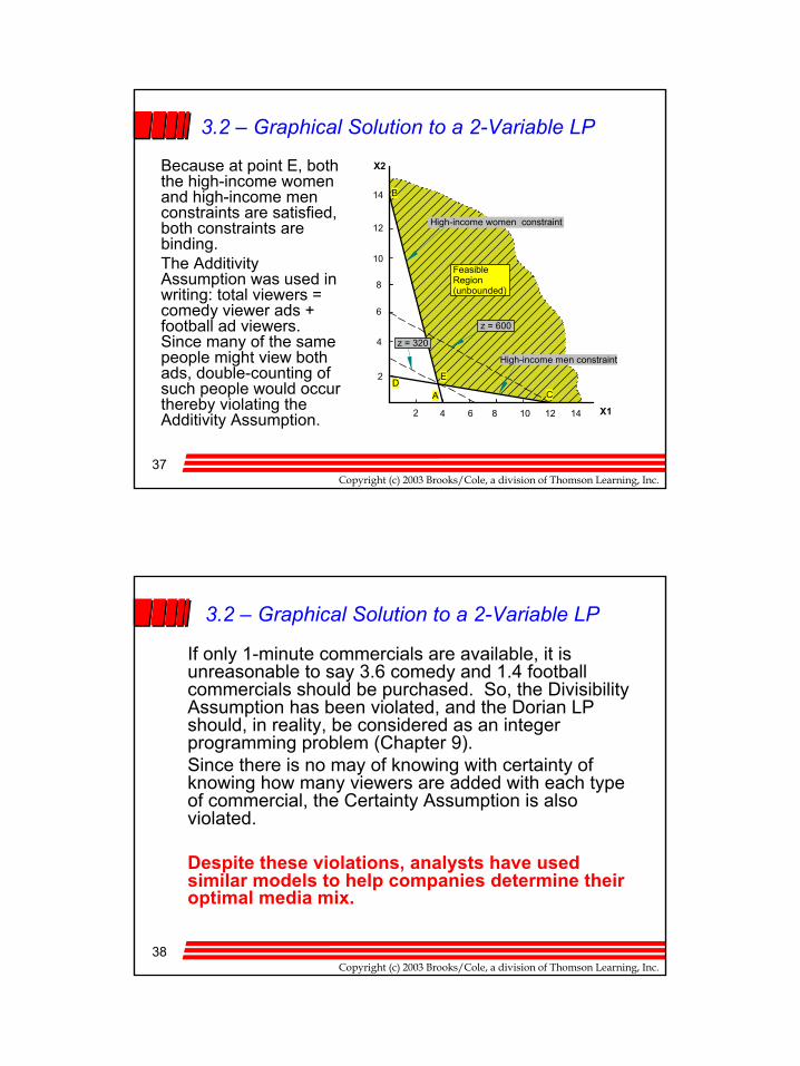
Because at point E, both the high-income women and high-income men constraints are satisfied, both constraints are binding.The AdditivityAssumption was used in writing: total viewers = comedy viewer ads + football ad viewers. Since many of the same people might view both ads, double-counting of such people would occur thereby violating the Additivity Assumption. X1

X2

2

4

6

8

10

12

14

2 4 6 8 10 12 14

z = 600

z = 320

A CD

E

B






If only 1-minute commercials are available, it is unreasonable to say 3.6 comedy and 1.4 football commercials should be purchased. So, the Divisibility Assumption has been violated, and the Dorian LP should, in reality, be considered as an integer programming problem (Chapter 9).Since there is no may of knowing with certainty of knowing how many viewers are added with each type of commercial, the Certainty Assumption is also violated.

Despite these violations, analysts have used similar models to help companies determine their optimal media mix.

20



The Giapetto and Dorian LPs each had a unique optimal solution. Some types of LPs do not have unique solutions.

• Some LPs have an infinite number of solutions (alternative or multiple optimal solutions).

• Some LPs have no feasible solutions (infeasible LPs).

• Some LPs are unbounded: There are points in the feasible region with arbitrarily large (in a maximization problem) z-values.



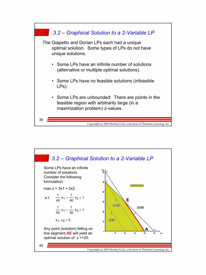
max z = 3x1 + 2x2

s.t.140

x1⋅160

x2⋅+ 1≤

150

x1⋅150

x2⋅+ 1≤

x1 x2 0≥,

Any point (solution) falling on line segment AE will yield an optimal solution of z =120.

Some LPs have an infinite number of solutions. Consider the following formulation:

X1

X2

10 20 30 40

1020

3040

50

Feasible Region

F50

60

z = 60

z = 100 z = 120

A

B

C

D

E

21



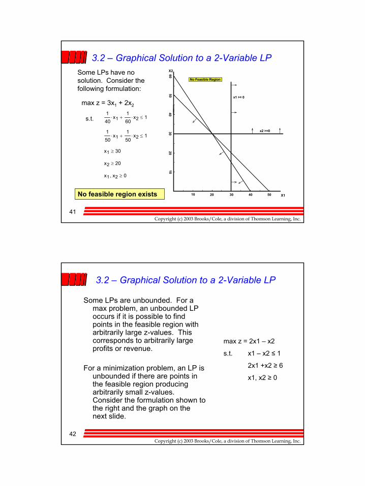
s.t.

max z = 3x1 + 2x2

140

x1⋅160

x2⋅+ 1≤

150

x1⋅150

x2⋅+ 1≤

x1 30≥

x2 20≥

x1 x2 0≥,

X1

X2

10 20 30 4010

2030

4050

No Feasible Region

5060

x1 >= 0

x2 >=0

No feasible region exists

Some LPs have no solution. Consider the following formulation:



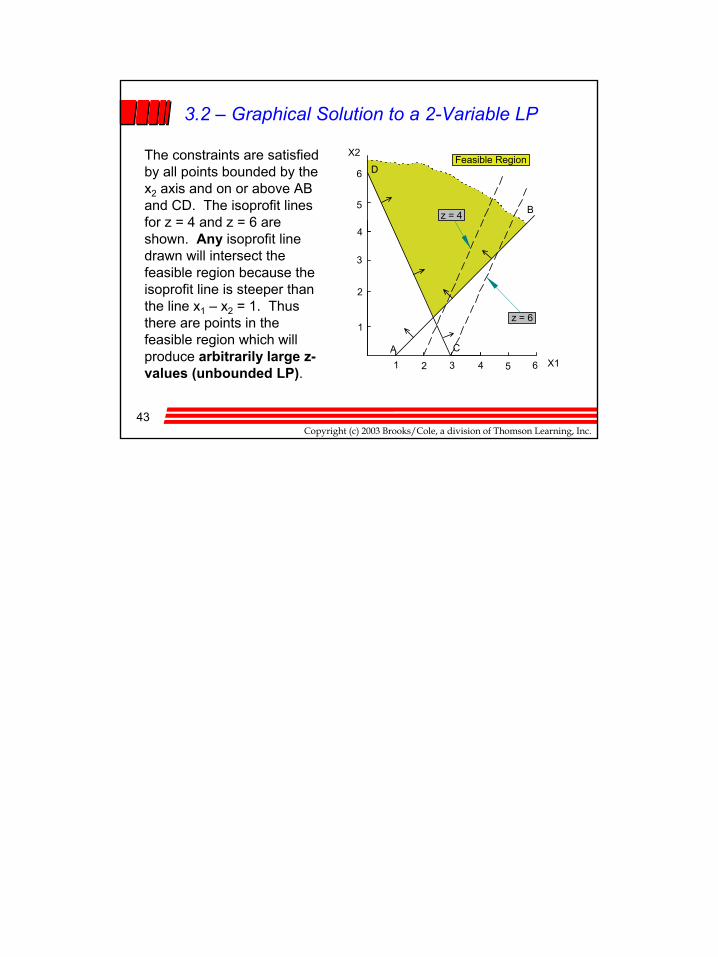
Some LPs are unbounded. For a max problem, an unbounded LP occurs if it is possible to find points in the feasible region with arbitrarily large z-values. This corresponds to arbitrarily large profits or revenue.

For a minimization problem, an LP is unbounded if there are points in the feasible region producing arbitrarily small z-values. Consider the formulation shown to the right and the graph on the next slide.

max z = 2x1 – x2

s.t. x1 – x2 ≤ 1

2x1 +x2 ≥ 6

x1, x2 ≥ 0

22



X11 2 3 4

1

2

3

4

X2

5

6

5 6A

B

C

Feasible Region

z = 4

z = 6

DThe constraints are satisfied by all points bounded by the x2 axis and on or above AB and CD. The isoprofit lines for z = 4 and z = 6 are shown. Any isoprofit line drawn will intersect the feasible region because the isoprofit line is steeper than the line x1 – x2 = 1. Thus there are points in the feasible region which will produce arbitrarily large z-values (unbounded LP).

chapter 3 introduction to linear programmingjyee/491.06/lectures/chapter03.pdf · chapter 3...

Documents