Chapter 3

RESEARCH PROCEDURES

The data for our test of a macro approach to estimating intrinsic

water quality benefits was gathered in 1576 personal interviews of a

national probability sample of persons 18 years of age and older. The

sample was designed and the interviews were conducted by the Roper Organ-

ization. Interviewing took place in two waves: 1289 people were interv-

viewed in late January - early February 1980 and 287 in March 1980.1

The

sampling plan was a multistage probability sample. Once an eligible person

was identified, as many as four attempts were made to arrange an interview.

Seventy-three percent of the individuals selected were ultimately interviewed.

A description of the sampling design is contained in Appendix V.

For the entire sample, the chances are 95 out of 100 that the results on

a particular question are within 2 to 3 percentage points of the results that

would have been obtained from a very large sample selected and interviewed

in a similar manner.

National surveys are very expensive to conduct. We were able to

minimize the costs of this experiment by taking advantage of an ongoing

survey. After the interview for the original survey was completed, the

interviewers administered our sequence of benefits questions. From the

respondents' perspective, the two interviews appeared as one long interview.

1 It was originally intended that all the interviewing would be donein the initial period, but the survey contractor had an unanticipatedshortfall in interviews which went unrecognized for a month. This neces-sitated further interviewing to bring the sample up to 1500.

3-2

While this procedure allowed us to have our instrument field tested in

a way that was completely satisfactory, budgetary constraints limited the

number of questions we could ask and prevented us from preparing a

set of briefing materials for the interviewers. Consequently, as will be dis-

cussed at length in later chapters, the percent of respondents who failed to give

the interviewers the amount they were willing to pay for the levels of

water quality was high, as was the percent who gave zero bids. In this

chapter we describe the context of the survey and the instrument. Sub-

sequent chapters discuss the reliability and validity of the responses

and the values people have for water quality. The final chapter presents

a plan for revising the procedures to improve the measures and increase

the response rate to the wtp questions.

Context

The RFF water benefits questions took about 10-15 minutes to

administer. They were preceded by a separate half-hour

survey on environmental issues which was conducted for another study.

Since the questions for this other study set the context for the water benefit

questions it is important to outline briefly their content and results.

3-3

We will discuss the possible biasing effect they may have had at a later

point in this report.

The environmental survey consisted of some 100 items which probed the

respondent's views about national priorities, environmental protection, the

regulation of risks, energy issues, values, and views about government and

the environmental movement. A number of these items were repeated from

earlier surveys for trend purposes. This survey sought to probe beneath

the respondent's presumed predisposition towards environmental protection

(as consistently shown by other national surveys) by asking questions

which: a) forced the respondent to rank order the environment among other

national priorities, b) measured concern about economic issues and energy

shortages, and c) which forced the respondent to choose between tradeoffs

(e.g. environment vs. growth or environmental quality vs. lower cost of

regulation). The questionnaire for the environmental survey which preceded

the benefits questions, including the background questions used for both

studies, is in Appendix IV.

When the respondents were forced to rank order problems in terms of

which should have the most government priority, "reducing pollution of air

and water" fell to sixth place (out of 10 problems) from the second place

position it held at the time of the original Earth Day in 1970. Responses

to other questions in the environmental survey showed the respondents were

extremely concerned about inflation, energy problems, and defense. Never-

theless, while the environment is apparently no longer viewed as a crisis

issue, overall support for environmental protection showed continued strength

2in the trend and tradeoff questions, a finding confirmed by subsequent surveys.

For a description of the findings of the environmental survey seePublic Opinion on Environmental Issues (Council on Environmental Quality, 1980).

3-4

The data from the environmental survey are part of our benefits data

file and were used in our analysis of the benefits data. The environmental

survey included several questions about water quality issues. The respondents

were asked:

1. How worried or concerned they are with "cleaning up our

waterways and reducing water pollution." Thirty-nine percent

said they were concerned "a great deal," and at the opposite

extreme 16 percent said they were concerned not much or not

at all about water pollution. (See Q.11c, Appendix IV for the

marginals and comparisons across other areas of concern in 1980).

2. Their judgment about the quality of the water in the "lakes and

streams in this area" on a self-anchored 11 step ladder for the

present, past (five years ago) and the future (five years from

now). Q.18-20. From this set of questions it is possible to

calculate their optimism or pessimism about change in local

water quality over time.

3. How far in miles the nearest freshwater lake and river large

enough for boating are from their home (Qs. 33a and b).

4. A series of questions on use of water (Qs. 58-66) For boating,

swimming and fishing in a freshwater lake or stream, respondents

were asked whether they had engaged in each activity in the past

two years, if so whether they did it within fifty miles of their

home, and how many times they did it during this time period.

We used these questions for our measures of recreational water use.

3-5

Water Pollution Ladder and Value Levels

The levels of water quality for which we sought WTP estimates are

"boatable," "fishable," and "swimmable." We described these levels in

words and depicted them graphically by means of a water quality ladder.

Use of these categories, two of which are embodied in the law mandating

the national water pollution control program, allowed us to avoid the

methodological problems we would have faced had we chosen to describe water

in terms of the numerous abstract technical measures of pollution. Although

the boatable-fishable-swimmable categories are widely understood by the

public, they did require further specification on our part to ensure that

people perceived them in a similar fashion.

We defined boatable water in the text of the question as an inter-

mediate level between water which "has oil, raw sewage and other things in

it, has no plant or animal life and smells bad" on the one hand and water

which is of fishable quality on the other. Fishable water covers a fairly

large range of water quality. Game fish like bass and trout cannot tolerate

water that certain types of fish such as carp and catfish flourish in.

In our pretests we initially ex-

perimented with two levels of fishable water -- one for "rough" fish like carp or

catfish and the other for game fish like bass -- but we were forced to

abandon this distinction because people were confused by it. We adopted a

single definition of "fishable" as water "clean enough so that game fish

like bass can live in it" under the assumption that the words "game fish"

and "bass" had wide recognition and connoted water of the quality level

Congress had in mind. Swimmable water appeared to present less difficulty

3-6

for popular understanding since the enforcement of water quality for

swimming by health authorities has led to widespread awareness that

swimming in polluted water can cause sickeness to humans.

Because WTP questions have to describe in some detail the conditions

of the "market" for the good they are inevitably longer than the usual

survey research questions. Respondents quickly become bored and restless

if material is read to them without giving them frequent opportunities to

express judgments or to look at visual aids. We designed the RFF instrument

to be as interactive as possible by interspersing the text with questions

which required the respondents to use the newly described water quality

categories. We also handed them a water quality ladder card which was

referred to constantly during the sequence of benefits questions.

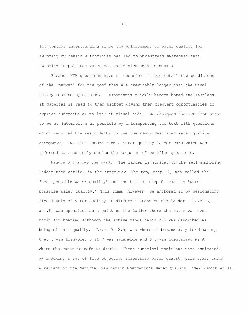
Figure 3.1 shows the card. The ladder is similar to the self-anchoring

ladder used earlier in the interview. The top, step 10, was called the

"best possible water quality" and the bottom, step 0, was the "worst

possible water quality." This time, however, we anchored it by designating

five levels of water quality at different steps on the ladder. Level E,

at .8, was specified as a point on the ladder where the water was even

unfit for boating although the active range below 2.5 was described as

being of this quality. Level D, 2.5, was where it became okay for boating;

C at 5 was fishable, B at 7 was swimmable and 9.5 was identified as A

where the water is safe to drink. These numerical positions were estimated

by indexing a set of five objective scientific water quality parameters using

a variant of the National Sanitation Foundatin's Water Quality Index (Booth et al.,

B

Figure 3.13-7

(WATER QUALITY LADDER CARD) #684

BEST POSSIBLEWATER QUALITY

10

9

8

7

6

5

4

3

2

1

0

SAFE TO DRINK

SAFE FOR SWIMMING

WORST POSSIBLEWATER QUALITY

GAME FISH LIKE BASS CAN LIVE IN IT

OKAY FOR BOATING

3-8

1976; McClelland, 1974). The method is described in Appendix II.

Although this is necessarily a tenuous scaling procedure, it yielded a

set of positions which appear reasonable. Our pretests showed that respondents

did not seem to be sensitive to changes of one or two rungs in the location

of the water quality levels along the scale.

We introduced the market and the ladder in the following manner:

This last group of questions is about the quality of water inthe nation's lakes and streams. Comgress passed strict waterpollution control laws in 1972 and 1977. As a result manycommunities have to build and run new modern sewage treatmentplants and many industries have to install water pollutioncontrol equipment.

Here is a picture of a ladder that shows various levels ofthe quality of water. (HAND RESPONDENT WATER QUALITY LADDER CARD)Please keep in mind that we are not talking about the drinkingwater in your home. Nor are we talking about the ocean. We aretalking only about freshwater lakes, rivers and streams thatpeople look at and in which they go boating, fishing and swimming.

The top of the ladder stands for the best possible quality ofwater, that is, the purest spring water. The bottom stands forthe worst possible quality of water. Unlike the other ladderswe have used in this survey, on this ladder we have markeddifferent levels of the quality of water. For example . . . .(POINT TO EACH LEVEL: E, D, C, AND SO ON, AS YOU READ STATEMENTSBELOW)

Level E (POINTING) is so polluted that it has oil, rawsewage and other things in it, has no plant or animallife and smells bad

Water at level D is okay for boating but not for fishingor swimming

Level C shows where rivers, lakes and streams are cleanenough so that game fish like bass can live in them

Level B shows where the water is clean enough so thatpeople can swim in it safely

And at level A, the quality of the water is so good thatit would be possible to drink it directly from a lake orstream if you wanted to

3-9

We thus defined the environmental good as freshwater lakes, rivers and

streams and distinguished it from drinking water and salt water. We

specifically invoked visual values as well as the active use values of

boating, fishing and swimming.

Our intention was to obtain a WTP estimate for national water quality.

In order to get the respondent to think about the national situation the

interviewer next asked:

Now let's think about all of the nation's rivers, lakes andstreams. Some of them are quite clean and others are moreor less polluted. Looking at this ladder, would you say thatall but a tiny fraction of the nation's rivers, lakes andstreams are at least at level D in the quality of theirwater today or not?

Strictly speaking, the law mandates water cleanup for all freshwater bodies.

We substituted "all but a tiny fraction" for "all" in this and the following

questions because we did not want to unnecessarily complicate the issue by

having respondents speculate about the impossibility of every portion of every

water body in the nation being at a certain water quality level at all times. Six

out of ten respondents agreed that today all but a fraction of the nation's

freshwater bodies are at level D while 17 percent were not sure and 20

percent felt that level had not yet been reached.

The next section of the instrument was meant to introduce the respondent

to two things: 1) the fact that water pollution control costs money and

2) that the level of cleanup is a matter of preference. We did this by

asking the following question:

3-10

81. As you know it takes money to clean up our nation's lakes andrivers. Taking that into account, and thinking of overallwater quality where all but a tiny fraction of the nation'slakes and rivers are at a particular level, which level ofoverall water quality do you think the nation should plan toreach within the next five years or so -- level E, D, C, B, or A?

Eighty-five percent chose a goal of fishable or better (C, B, or A) while

57 percent chose swimmable or better (B or A).

Payment Vehicle

We used two principal criteria to choose our payment vehicle. The

first is realism -- the vehicle should match the way people actually pay

for higher water quality as closely as possible. The second criteria is

conservativism -- every effort should be made to avoid a false overstatement

of willingness to pay. Conservativism in question design is important be-

cause unless respondents are made to pay the amounts they offer, WTP

studies are inevitably hypothetical in character. The bias associated

with hypothetical situations is towards overstating the amount the person

is willing to pay3although the amount of overstatement is not necessarily

large (Bohm, 1972) and is sometimes nonexistent (Davis, 1980). Given many

economists' fear that the WTP methodology is biased upward, the findings

of WTP questions will be credible only if every effort is made to avoid

this bias. Our procedure was to design our instrument so that, whenever

possible, any bias present is toward lowering rather than raising

the WTP amount.

We selected annual household payment in higher prices and taxes as

our payment vehicle because this is the way people pay for water pollution

control programs. A portion of each household's annual federal tax payment

See Chapter 4.

3-11

goes towards the expense of regulating water pollution and providing con-

struction grants for sewage treatment plants. Local sewage taxes pay for

the maintenance of three plants. Those private users who incur pollution

control expenses, such as manufacturing plants, ultimately pass much or

all of the cost along to consumers in higher prices. This payment vehicle

is conservative because:

Ever since the passage of Proposition 13 in California in 1977,

opposition to the current level of taxes is a commonly expressed

attitude which is socially acceptable (even normative). Concern

about inflation was the nation's "most important problem" according

to polls taken at the time of the RFF survey. Thus we can assume

the words "taxes and higher prices" will not be taken lightly

by our respondents and may, for some, have a highly charged negative

connotation.

By asking for the annual amount a person is willing to pay instead of

for a monthly amount, we avoid the possibility of an “easy payment

plan" underestimation.

Starting Point

Our review of the literature on micro WTP studies and on survey research

more generally, identified starting point bias as a particularly serious

problem for our study. Because of this we developed and tested an

alternative to the commonly used bidding game WTP method. In this section

we outline the problems presented by the bidding game technique and describe

our alternative procedure -- the payment card method.

3-12

The widely used bidding game format for WTP studies uses a sequence

of yes/no questions and normally requires the interviewer to begin the

bidding process by offering an initial amount. The subsequent bids flow

from that point, albeit in either direction. If the amount presented

influences the respondent's final bid in some systematic way -- starting

point bias -- we have a serious problem.

There are a priori reasons for suspecting such a bias in this type

of situation. The tendency of respondents to give a socially desirable

answer (Edwards, 1957; Dohrenwend, 1966; Phillips and Clancy, 1970, 1972)

or to acquiesce when confronted with questions using a yes/no agree or

disagree format (Couch and Keniston, 1960; Campbell et al., 1967; Carr,

1977; Jackman, 1973; and Phillips and Clancy, 1970) is well documented.

Accordingly, when valuing a public good like water quality, a respondent

may be reluctant to reject a starting bid even when it is higher than he

is willing to pay for fear of appearing cheap or lacking a social con-

science (social desirability effect) and/or because of a tendency on the

part of the respondent to agree with suggestions offered by the interviewer

(acquiescence effect).

In practice, strong starting point effects have been found by some

researchers doing micro WTP studies (Rowe et al., 1979) although other

researchers have not found them (Thayer, et al., forthcoming; Brookshire,

et al., 1979; Brookshire et al., 1980). Where starting point bias has

been discovered, the effect of higher starting points is to raise the

mean WTP amount.

3-13

The acquiescence effect shows a strong relationship with education --

people with less education are much more likely to acquiesce than those

with more education (Jackman, 1973). This introduces a further bias. If

we assume, as studies have shown, that WTP varies by income level and that

income is correlated with education, then the potential for an education/ WTP

interaction effect is strong when a single starting point is used for the

entire sample. When choosing a single starting point, the researcher needs

one that will be below the expected mean for the entire sample, but not too

far below or the process of bidding upward to find the maximum WTP amount will be

too laborious. An initial bid which meets this requirement for the entire

sample can be expected to be below the mean for people in the $15-25,000

range, close to the mean of the real bid for someone in the $8,000-14,999

income range and above the real mean bid for those with lower incomes. Since

many people in the lower income range will also have low educations, in this

situation they are likely, by the operation of the acquiescence effect, to

overbid for the good in question. The reverse is less likely to happen

for those with an income above $25,000 because their educational level is

higher (on the average) and therefore their propensity for acquiescence in

the interview situation is lower. Thus even if the overall starting bias

described earlier is not present, overstatement of benefits by lower income

people will bias the WTP amounts upwards.

A further problem with the bidding game technique is that the process

of iterating from a starting point to a final WTP amount can be tedious

if the starting point lies some distance from the respondent's real WTP

amount. If the range is narrow -- such that most respondents, for example,

3-14

value a certain good at between $1 and $5 per month on their utility bill

-- and if the increments are fairly large -- say $1 -- then the process

can be accomplished fairly efficiently. When this is not the case, the

length of the iteration process can alienate respondents or cause them

to cease bidding before reaching their maximum amount.

The problems with the bidding game approach enumerated above are

exacerbated for payment vehicles like ours which engender large bids (be-

cause they ask for an annual household amount for national water quality)

and which are strongly income dependent (owing to the income tax component

of the vehicle). Moreover, it seems questionable that the bidding game

technique can be used reliably by professional interviewers such as ours

who are spread across the country and cannot be personally instructed in

its use. For these reasons we developed our payment card technique to

elicit the respondent's WTP amounts.

In this technique the respondent is given a card which contains a menu

of amounts which begin at $0 and increase by a fixed interval until an

arbitrarily determined large amount is reached. When the time comes to

elicit the WTP amount, the respondent is asked to pick a number off the

card (or any number in between) which "is the most you would be willing to

pay in taxes and higher prices each year" (italics in the original) for a

given level of water quality. The question asks people to give us the

highest amount they are willing to pay and we accepted their answer as

representing such an amount. In our pretesting we tried asking people if

3-15

they would be willing to pay a higher amount than the one they picked and

found some people resented being "pushed" once they had settled on an amount.

Others would give us a higher amount but in such a way that we suspected

they were acquiescing to interviewer pressure rather than revealing their

true consumer surplus.

The payment card has two special features:

1. It is anchored. In our initial pretests we found the respondents

had considerable difficulty in determining their willingness to pay when

we used a card which only presented various dollar amounts. A number of

them expressed embarrasment, confusion, or resentment at the task and some

who gave us amounts indicated they were very uncertain about them. We

determined that the problem lay with the lack of benchmarks for their

estimates. People are not normally aware of the total amounts they pay for

public goods even when that amount comes out of their taxes, nor do they

know how much they cost. Without a way of psychologically anchoring their

estimate in some manner they were not able to arrive at meaningful estimates.

They needed benchmarks of some kind which would convey sufficient infor-

mation without biasing their WTP amounts. We reasoned that the most ap-

propriate benchmarks for WTP for water pollution control would be the amounts

they are already paying in higher prices and taxes for other non-environmental

public goods. We identified amounts on the card for several such goods and

conducted further pretests. These showed the benchmarks made the task

meaningful for most people.

The use of payment cards with benchmarks raises the possibility of

information bias. Are the respondents who gave us amounts for water pollution

3-16

control using the benchmarks for general orientation or are they basing their

amounts directly on the benchmarks themselves in some manner? In the former

case people would be giving us unique values for water quality; in the latter

case they would be giving us values for water quality relative to what they

think they are paying for a particular set of other public goods. If the

latter case holds and their water quality values are sensitive to changes in

the benchmark amounts or to changes in the set of public goods identified on

the payment card, their validity as estimates of consumer surplus for water

quality are suspect.

We designed our study to test for information bias due to the benchmarks.

Four different versions of the payment cards were prepared and administered

to approximately equivalent sub-samples. Figures 3.2 shows the cards given to

the lower-medium income respondents ($10,000-14,999 annual family income)

for the A, B, C, and D versions. These versions varied as follows:

A Benchmarks are shown for the amounts we estimated the averagehousehold of that income level contributes to the space program,highways, public education and defense.

B The same four public goods and amounts as on A plus police andfire protection.

C The same four public goods used in version A were shown, but foramounts 25 percent higher than on version A.

D The same four public goods and amounts as in Version A, plusthe estimated amount for water pollution control.

We added the police and fire good in version B to see if the insertion

of a new item in the dollar range where water pollution benefits estimates

were likely to fall would affect those estimates. Version C seeks to test

whether the actual amounts shown for the benchmarks affect the water pol-

lution WTP amounts. We purposely omitted environmental goods in each of the

3-17

Figure 3.2 PAYMENT CARDS FOR VERSIONS A, B, C, D FOR PEOPLE WITH FAMILY INCOMES OF $10,000-14,999

3-18

first three versions to avoid having people would tell us what they think

they should give rather than what they actually want to pay. In version D

we added our estimate of what average households are actually paying for

water pollution control to see whether this information actually does

bias the WTP amounts.

Deriving the dollar estimates for each of our benchmark public goods

was a difficult task particularly because we needed them for four income

levels as well (see below). A detailed description of our procedures is

given in Appendix III. We are satisfied that the estimates are sufficiently

close approximations to suffice for this test. If it turned out that

people's WTP amounts are very sensitive to the benchmark amounts, then much

more effort would be required to improve the accuracy of these estimates.

2. It is income adjusted. For the reasons stated earlier, the amounts

people are actually paying for water pollution control vary by income. This

is also the case for the other public goods which we used as benchmarks.

We corrected for this by developing benchmark goods estimates for four

different income categories: I) family income under $10,000; II) $10,000-

14,999; III) $15,000-24,999; IV) $25,000 and above. (Appendix I gives our

public goods estimates for each of these income categories). Each inter-

viewer therefore had four different payment cards for each of the A, B, C,

and D forms. At the appropriate point in the interview the interviewer gave

the respondent the payment card for his or her income category. (A question

on income preceded the water quality benefits questions.) For the 10 percent

of respondents who refused to divulge their income our procedure was to give

them the income card for income level IV, the highest income level as people

with higher incomes are more likely to refuse to divulge their income.

3-19

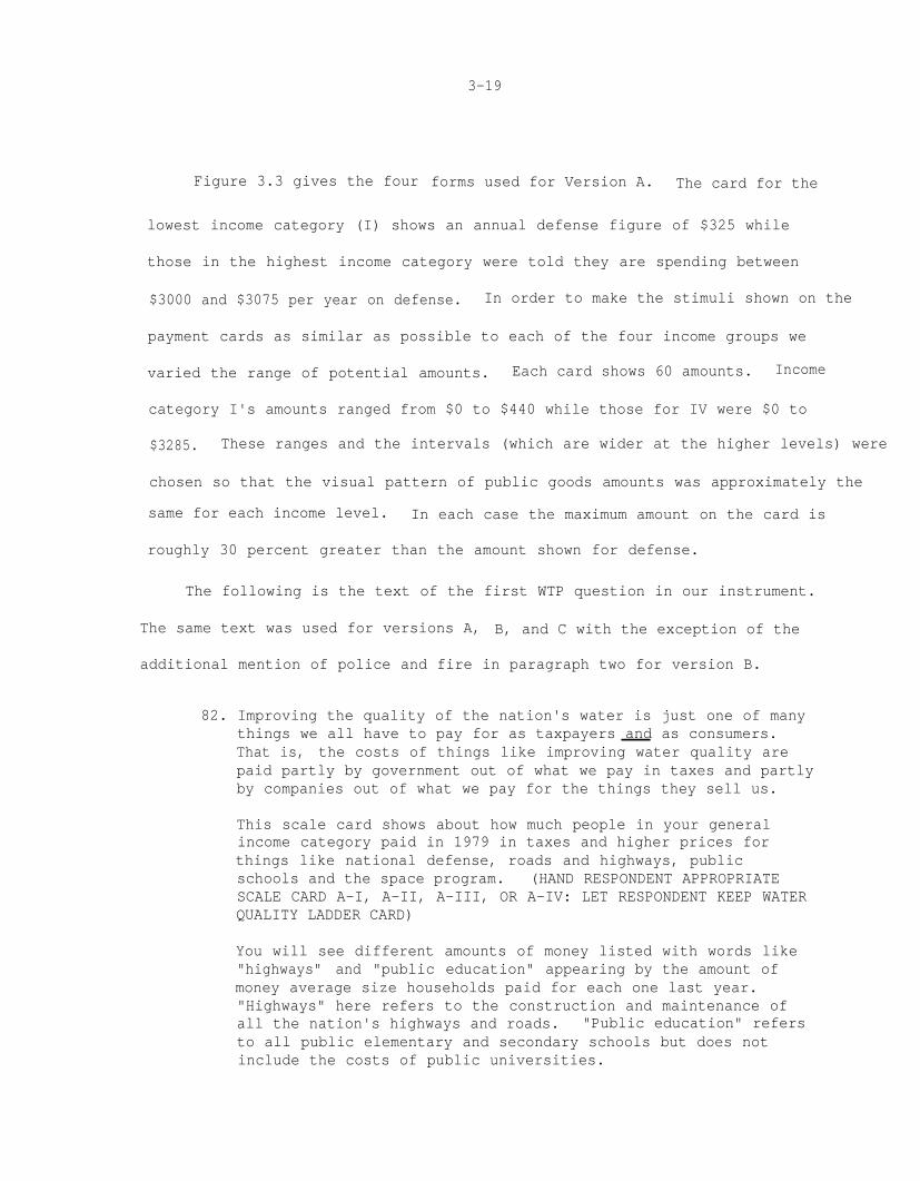
Figure 3.3 gives the four forms used for Version A. The card for the

lowest income category (I) shows an annual defense figure of $325 while

those in the highest income category were told they are spending between

$3000 and $3075 per year on defense. In order to make the stimuli shown on the

payment cards as similar as possible to each of the four income groups we

varied the range of potential amounts. Each card shows 60 amounts. Income

category I's amounts ranged from $0 to $440 while those for IV were $0 to

$3285. These ranges and the intervals (which are wider at the higher levels) were

chosen so that the visual pattern of public goods amounts was approximately the

same for each income level. In each case the maximum amount on the card is

roughly 30 percent greater than the amount shown for defense.

The following is the text of the first WTP question in our instrument.

The same text was used for versions A, B, and C with the exception of the

additional mention of police and fire in paragraph two for version B.

82. Improving the quality of the nation's water is just one of manythings we all have to pay for as taxpayers and as consumers.That is, the costs of things like improving water quality arepaid partly by government out of what we pay in taxes and partlyby companies out of what we pay for the things they sell us.

This scale card shows about how much people in your generalincome category paid in 1979 in taxes and higher prices forthings like national defense, roads and highways, publicschools and the space program. (HAND RESPONDENT APPROPRIATESCALE CARD A-I, A-II, A-III, OR A-IV: LET RESPONDENT KEEP WATERQUALITY LADDER CARD)

You will see different amounts of money listed with words like"highways" and "public education" appearing by the amount ofmoney average size households paid for each one last year."Highways" here refers to the construction and maintenance ofall the nation's highways and roads. "Public education" refersto all public elementary and secondary schools but does notinclude the costs of public universities.

3-20

Figure 3.3 PAYMENT CARDS FOR INCOME LEVELS I-IV FOR VERSION A

3-21

I want to ask you some questions about what amounts of money,if any, you would be willing to pay for varying levels ofoverall water quality in the nation's lakes, rivers and streams.Please keep in mind that the money would go for sewage treatmentplants in communities through various kinds of taxes (such aswithholding taxes, sales taxes and sewage fees) and for pollutioncontrol equipment the government would require industries toinstall, thus raising the prices of what they make.

At the present time the average quality of water in the nation'slakes, rivers and streams is at about level D on the ladder.(POINT TO LEVEL D ON WATER QUALITY LADDER CARD) If no more moneywere spent at all tomorrow on water quality, the overall qualityof the nation's lakes and rivers would fall back to about level E.(POINT TO LEVEL E) People have different ideas about how importantthe quality of lakes, rivers and streams is to them personally.Thinking about your household's annual income and the fact thatmoney spent for one thing can't be spent for another, how much doyou think it is worth to you to keep the water quality in the nationfrom slipping from level D back to level E? That is, which amounton this scale card, or any amount in between, is the most youwould be willing to pay in taxes and higher prices each year tokeep the nation's overall water quality at level D where virtuallyall of it is at least clean enough for boating? If it is notworth anything to you, please do not hesitate to say so.

Several aspects of question 82 bear comment. For the purpose of

convenience we started the process of demand revelation with the present level

of national water quality (boatable) and asked respondents to value a

reduction in this quality to level E, non-boatable. (In subsequent

questions we had them value hypothetical increases from boatable to fishable

and then swimmable.) In this question we expanded the account given in the

previous questions about how their money would be used and reinforced the

ideas that the WTP amount would be coming out of their annual income and its

use for this purpose would preclude other uses of the money. At two points

in this question we legitimated a low or zero WTP amount in an effort to

minimize the social desirability effect. We noted that "people have dif-

ferent ideas" about the importance of water quality to them personally

3-22

and at the conclusion of the question we stated: "If it is not worth

anything to you, please don't hestiate to say so."

The response categories which were supplied to the interviewers for

this question were:

Write in amount: $

Depends (voluntary)

Not sure

Not worth anything

Through a misunderstanding the survey contractor did two things

which may have biased the results. First in this and the next

question, those who responded "not worth anything" -- in effect a $0 bid

-- were not asked how much they were willing to pay for water of higher

quality. Instead, the interviewers skipped directly to the last question.

Presumably most of the people who valued boatable water at $0 were generally

unwilling to pay for water pollution control of any kind and would also have

valued fishable and swimmable quality water at $0. Our analysis of the

views of these people about water pollution and environmental quality sug-

gests that this conjecture is probably true for most of them. But some of

them may indeed only value water nationwide when it reaches the fishable

and/or swimmable quality levels. If so, they would have given a WTP amount

greater than $0 for the higher levels, if they had the opportunity, despite

their $0 bid for the lower level. Second, when the data were keypunched,

the contractor restricted the WTP amounts to three colums, thereby limiting

the maximum WTP amount to $999. For versions A, B, C combined, 43 People

3-23

were recorded as WTP this maximum amount for level B. We have no way of

knowing how many of these people actually valued water quality at an

amount higher than this. It is our judgment that both these errors have

had only a minor effect on our estimates. The direction of the

bias is, of course, conservative.

The next question sought the respondents' WTP for fishable

level C.

resulting

water,

83. As I mentioned earlier, almost all of the rivers and lakesin the United States are at least at level D in water quality.What do you think it is worth to you not only to keep themfrom becoming more polluted but also to raise their overallquality to level C? That is, including the amount you justgave me, which amount on the scale card is the most you wouldbe willing to pay in taxes and higher prices each year to raisethe overall level of water quality from level D to level C wherevirtually all of it would at least be clean enough for fishlike bass to live in?

The final WTP question used the same format for swimmable water,

level B.

84. What about getting virtually all of the nation's lakes andrivers up to level B on the ladder? Including the amountsof money you have already given me, which amount on thescale card is the most you would be willing to pay in taxesand higher prices each year to make almost all the nation'slakes, rivers and streams clean enough so that people couldswim in them?

In two of the versions, A, and C, we asked the respondents to evaluate

the amount of information we provided them about the WTP exercise. We were

precluded from asking this of all the respondents because of severe con-

straints on the length of the questionnaire.

3-24

85. Finally, in terms of your being able to decide exactly howmuch you, yourself, would be willing to pay as a taxpayerand consumer for better water quality, would you say in thelast few questions we gave you more than enough information,about enough information, not quite enough, or not enoughinformation at all?

CHAPTER 4

CONTROL FOR BIASES

Prior to discussing our findings it is necessary to examine the

character of the data we have gathered. To what extent are they free from

bias? The micro willingness-to-pay literature has devoted considerable

attention to the potential biases, their effect and how they may be overcome

(Schulze, et al., 1980). Table 4.1 lists these potential biases and several

others which we believe to be important.

Table 4.1

POTENTIAL BIASES IN WILLINGNESS TO PAY STUDIES

General Sampling

Strategic Sample

Hypothetic Response Rate

Instrument Interview

Starting Point Item non-response

Payment Vehicle Interview Procedure

Information Interviewer

Order

4-2

GENERAL BIASES

Strategic and hypothetic are the two sources of bias of greatest

fundamental concern to economists who wish to evaluate the validity of

willingness to pay surveys.

Strategic Bias

Its Nature

Strategic bias is the attempt by respondents to influence the outcome

of a study in a direction which favors the respondents' interests by

deliberately misrepresenting their demand for a good. In 1954, Paul

Samuelson argued on free-rider grounds that a person would be motivated

to "pretend to have less interest in a given collective consumption

activity than he really has" and despaired of finding a way of overcoming

this problem (1954). Samuelson assumes

that the individual would believe he or she would have to pay the amount

he or she declares as being willing to pay. If this assumption is relaxed,

as seems reasonable, many economists believe an incentive to overestimate

consumption would be prevalent (Freeman,19796:88). For example, take a

survey whose respondents believe the mean WTP amount for all respondents

will influence the government's provision of a public good and that they

will not be obligated to pay their WTP amount. If they value the good,

the respondents may attempt to raise the mean (and impose their preference)

by overstating their willingness to pay. Robert Crandall seems to have

this kind of situation in mind when he wrote: "Such surveys (consumer

1See Kutz (1975) for the the theoretical conditions necessary for

successful strategic behavior.

4-3

surveys) are always biased when the respondent knows that he or she does

not have to write a check to confirm the answer" (Crandall, 1979). Conversely,

those who do not value the good very highly but assume that many others do,

may underestimate their willingness to pay in order to lower the mean and

bring it closer to their actual willingness to pay.

Empirical attempts to test for strategic bias in willingness to pay

studies and laboratory experiments have consistently failed to find it

(Brookshire, et al., 1979:22-23; V.L. Smith, 1977). A much cited challenge

to the notion that strategic bias can be overcome in WTP studies is an

experiment conducted by Peter Bohm. In one of the few attempts to compare

hypothetical WTP questions with the results from identical non-hypothetical

situations, Bohm (1972) conducted an experiment where participants bid

for the opportunity to see a closed circuit television program. He ran

six different versions of the experiment most of which systematically intro-

duced incentives to act strategically in a situation where the respodent

actually had to pay their bids. Only one version, Group VI, gave bids

which were significantly different from any of the others. Since this

group was told that they would not actually have to pay what they bid,

Bohm draws the conclusion that "when no payments and/or forced decisions

are involved people will act in an irresponsible manner" (Bohm, 1972:125).

In other words, when the consequences for respondents are hypothetical

they will overbid. Careful examination of Bohm's study shows that this

conclusion is unwarranted:

4-4

1. Out of five comparisons, Group VI's mean bid was significantly

higher in only one case (Group III).

2. Group VI was higher in income than the other groups which may

account for the size of its mean payment.

3. Group V also did not have to pay its bid. If strategic

bias was operative, there are reasons to think that this group

should have had the highest bid of all, but it did not.

4. Unlike the other groups, Group VI had one high outlier (at 50

where the median bid was 10) which raised its mean bid considerably.

When the outlier is removed, its mean payment is reduced from 10.19 to 9.45

Kroner and the difference between Group VI and Group III drops below the

.05 level of significance. It would appear that only one person

2of 54 may have acted "irresponsibly."

The incentives to misrepresent preferences are minimal in most WTP

surveys because respondents lack either the information necessary to act

strategically or the incentive to do so because respondents do not believe

they will be directly affected by the study's outcome. Although respondents

take valuation questions seriously, most do not think their responses will have

an immediate effect on policy nor should they since policy has rarely, if ever,

been set in this manner. The now conventional wisdom on strategic bias in WTP

surveys was recently summarized by Feenberg and Mills in their recent review of

water benefit analysis. They concluded, "It is unlikely that the problem is

serious" (Feenberg and Mills, 1980).

2We do not believe the one person acted strategically since an incentive

to overbid in this situation was not apparent although our colleague, CliffordRussell, believes this to be an example of strategic bias.

4-5

Our instrument was designed to minimize possible incentives to engage

in strategic behavior. No policy outcome was mentioned in the instrument

nor were respondents told how their WTP amounts would be used. Even if

respondents inferred that the study's findings are intended for government

guidance in some way, most would be aware of the indirect connection between

such a study and the actual process by which tax rates and prices are

determined. _On a priori grounds, therefore, we would not expect strategic

bias to affect our results.

( continue)

4-6

Distribution Tests for Strategic Bias

Apart from specific experimental tests, two possible indicators of

strategic bias, neither of them formalized, have been suggested, A

distribution test was first proposed by Brookshire, Ives and Schulze (1976).

They hypothesized that the distribution of the WTP amounts (in their case,

bids) will be normal when strategic bias is absent. If it is present, they

predict a "flattened" distribution. They examined the distribution of

responses for their study, which involved the aesthetic benefits of

foregoing the siting of a power plant near Lake Powell, and concluded on

the basis of observation that since the distribution was "not flat,"

strategic behavior was unlikely.

This distribution test has several weaknesses.

1. Even if we accept the notion that non-strategically biased

distributions should be normal it is impossible for most WTP

distributions to pass the standard statistical tests for

normality such as the Komogorov-Smirnov test. These tests

assume that each data point has an equal probability of being

chosen, but since respondents tend to choose favorite numbers

(e.g., 5, 10, 20, 25 rather than 6, 11, 22, etc.), the resulting

distribution is always too lumpy to pass the test even though

the distribution may appear to approximate a normal distribution.

2Clifford Russell has recently called our intention to a groupeddata normality test (Burlington and May, 1958:180-181) which may be anappropriate normality test for these kinds of data.

4-7

2. The expectation that strategic behavior will flatten an

otherwise normal (or approximately normal) distribution is

well founded, but only if the distribution of those who value

the public good in question is normally distributed. In certain

situations there is reason to doubt that non-biased WTP amount

distributions will be normal. Imagine a population, most

of whom are either environmental enthusiasts or enthusiasts

for industrial growth at the lowest possible cost. If they

all act strategically,

flat distribution with

lating at the high end

end.

we will get a bi-modal rather than a

the environmentalists' amounts accumu-

and the industrial enthusiasts' at the other

3. Since income is the primary deterrent of willingness to pay

and since the distribution of income more clearly approximates

3a log normal curve than the normal curve. In the absence of

strategic bias, the distribution one would expect in this

situation would be closer to a log-normal than a normal

distribution.

Figure 4.1 gives the distribution of the WTP amounts for fishable (level C)

water for questionnaire versions A, B, and C combined.4

the distribution is

3According to O'Brien (1979:855) the log-normal distribution is somewhat

more skewed than the distribution of income in the United States.

4Unless otherwise specified, we will normally combine the results for

three versions, for reasons to be explained below. Whenever we report theresults for one level, we will use C, fishable water. Unless otherwisespecified, the results for the other levels (boatable, swimmable) parallelthose for fishable.

4-8

Figure 4.1

Frequency

300

270

240

210

180

150

120

80

30

DISTRIBUTION OF WTP AMOUNTS FOR FISHABLE WATERFOR VERSIONS A, B, C COMBINED INCLUDING ZERO AMOUNTS

$ 0-60 61-180 181-300 301-420 421-540 541-660 661-750 781-900 901-999

4-9

dominated by the WTP amounts in the lowest category, $0-60. Of these,

more than half are zero bids. The high occurrence of zero bids is one of

the two major problems with our method revealed by our experiment (the

other being the relatively high percent of people who failed to give any WTP

amount). It is a problem because it seems likely that most of those who

gave zero bids actually have a greater than zero value for water quality

and would be willing to pay some amount, however small, for water pol-

lution control if we had an improved way of eliciting their true preferences.

By probing zero responses, other studies have found that some of those who

give zero WTP amounts do so to protest some aspect of the interview

situation. This is undoubtedly the case in our situation, but we were

( continue )

4-10

unable, for the reasons discussed in Chapter 3, to probe our zero bidders to learn

the reasoning behind their amounts. (We discuss the problem of zero bidders in

detail later in this chapter under item non-response bias.) Since we are unable to

separate the "real" zero payers from the protest zero payers, our subsequent analysi

includes all those who gave zero amounts. By doing this we bias our findings downwa

by some indeterminate factor. However, for the sole purpose of examining

the distribution of the WTP amounts, we recalculated the distribution

leaving out all the zero amounts. The revised distribution is given in

Figure 4.2.

1. At the upper end the distribution falls off until the highest

category where it increases. This is caused in large part by

the arbitrary $999 upper limit to our WTP amounts. Since most of those who

gave this amount are in our highest income category, we believe that

if the $999 constraint had not been introduced at the keypunching

stage, the distribution would have tailed off gradually.

2. The overall shape of the distribution is not flat. It ap-

proximates a log normal distribution, a distribution similar

to that reported by Brookshire, et al. (1976) in their Lake

Powell study, and to the distribution of income in the United

States. Since income is a strong predictor of people's

willingness to pay for water quality, as we will see in Chapter 5,

we conclude that the distribution does not suggest strategic

bias.

4-11

Figure 4.2

Frequency

160

140

120

100

80

60

40

20

DISTRIBUTION OF WTP AMOUNTS FOR FISHABLE WATERFOR VERSIONS A, B, C COMBINED EXCLUDING ZERO AMOUNTS

$1-60 61-180 181-300 301-420 421-540 541-660 661-780 781-900 901-999

4-12

A second method of testing the hypothesis that the distribtuion of WTP

amounts will be "flatter" than normal when strategic bias is present is implied by

Brookshire, et al. (1976) in their Lake Powell study when they make the following

statements:. . . false bids will be very large relative to the mean forenvironmentalists and zero for non-environmentalists wherebids are constrained to be non-negative (1976:328).

. . . if strategic behavior had been prevalent one wouldexpect a significant number of high bids relative to themean bid (1976:340).

This test also has its problems. First, and most important, we have no

objective way of identifying "false" values since the essence of the

problem of preference revelation is that "true value is subjective and

typically cannot be observed independently" (Freeman, 19796:97). Second,

the simple fact that environmentalists are willing to pay more than other

people for environmental goods (and non-environmentalists less) does

not necessarily imply strategic behavior on their part, especially when

the environmental good being valued is a broad one like the nation's water

quality. If environmentalists are true to their professed ideals, we

would expect them to be willing to pay more for water quality than those

of comparable income who are less committed to environmentalist ideals.

Bearing these problems in mind, the best we can do is to arbitrarily

define certain WTP amounts as inappropriately "high" or "low," relative to

the respondents' income level, and see if a) the percentage of people

who give bids of this kind is large enough to be troublesome and

4-13

b) if environmentalists and anti-environmentalists are disproportionately

represented among those who give such bids in such a way that the results

will be biased one way or the other.

Table 4. 2 divides those who gave us amounts for fishable water into

four groups:

1. Those who gave zero.

2. Those who gave "low" amounts which we define as any amount above

zero but equal to or lower than half the amount shown on the

respondent's payment card as the amount contributed to the space

program. For those in the lowest income group this is 1-6 dollars;

for those in the highest this is 1-53 dollars.

3. Those who gave "high" amounts which we arbitrarily define as any

amount equal to or greater than the amount shown for public education

on their card. This amount was $204 for the low income group and

S1695 for the high income group.

4. Those who gave an amount between the low and high extremes, who

we label "normal."

Eighty-three percent of those who gave amounts greater than Zero5

fall into our "normal" category. Those in the extreme categories are

divided, with 10 percent giving "high" amounts and 7 percent willing to pay

low amounts. We conclude that those at the extremes are relatively few in

number and rather evenly balanced.

The table also shows some of the characteristics of the people in each

of these groups. Comparing those in the low category with the normals, the

lows have a larger percentage of people in the highest income category

5Coding did not distinguish between zero and one dollar responses,

which were both coded as zero (or, in log responses, as one).

4-14

T a b l e 4 . 2PERCENT OF THOSE GIVING VARIOUS LEVELS OF PAYMENT

WHO BELONG TO CERTAIN DEMOGRAPHIC AND ATTITUDINAL CATEGORIES

Amount Willing to Pay for Fishable Water (level C)'

$0 "LOW" “Normal” “High” Cave No Amount

Maximum N = 2

A

B

C

D

E

F

High Tucome3

Low Education:HighSchool and Below

Age 65 and Older

High on Environ-mental Sca le (2 -4 )

Very Concerned AboutWater Pollution

Use Water forRecreation

(183)4

13% (20)

78 (143)

25 (46)

6 (10)

30 (42)

34 (62)

(40) (447)

40% (16) 23%(101)

65 (26) 68 (275)

13 (5 ) 8 (38)

30 (11) 30 (144)

43 (40) 41 (196)

62 (25) 71 (334)

(52) (445)

48% (25) 16% (57)

43 (22) 73 (328)

0 (0 ) 20 (92)

62 (35) 20 (88)

65 (34) 38 (168)

83 (43) 49 (220)

1"Low" amounts are defined as any amount equal to or lower than half the amount people of the

respondents ’ income category were said to spend on space. “High” are amounts equal to or greaterthan the education amount given on the payment card. “Normal” are all amounts in between the lowand high amounts.

2Total N varies for each of the demographic and at t i tudinal categor ies .

3Def in i t ions o f var iab les arc as fo l lows : h igh income = 25t + / l ow educat ion = h igh schoo l or be low/

high on environmental scale = score o f 2 -5 on a sca le constructed f rom seven quest ions which var iesFrom -5 to +5 ; See Appendix for a Ful l descr ipt ion o f the sca le / water user = someone whohas fished, boated or swam in last two years.

4Note that these percents are each independent of the rows and colums. Here, 13

percent of those who are will ing to pay $0 have a “high” income.

4-15

($25,000 and above), and a lower percentage of users of freshwater for

recreation. Overall, they are as environmentally concerned as the

normals but are older, wealthier and somewhat less likely to use water for

recreation. This combination of characteristics does not suggest upward-biased

strategic behavior, although it is not inconsistent with free riding.

The highs are also higher in income than the normals. They are much

more likely to be high on our environmental scale -- and in their concern

about water pollution as a problem -- and somewhat higher in recreational

water use (See Chapter 5 for a description of these measures). Although we

would expect those who use and value water to place a higher value on it

through their willingness to pay, and while half of the highs are in the

highest income category and presumably can afford the amounts they said

they are willing to pay, these data are consistent with the idea that

some of these 52 people are overestimating their real willingness to

pay. Whether this is the result of deliberate calculation (strategic

bias) or unrealistic enthusiasm (hypothetical bias) cannot be determined.

We do know they are more than balanced by the 183 zero bidders.

4-16

Hypothetic Bias

Hypothetic bias is the "potential error induced by not confronting

the individual with the actual situation" (Schulze, et al., 1980). In a situation

influenced by hypothetic bias people are so far removed from the actual

situation that they do not have "genuine" opinions. Perhaps they are being

asked about something which is so far removed from their experience and

interests that they are indifferent to the public good. Alternatively, they

may have sufficient interest or potential interest in the topic but the

subject of inquiry is not specified in sufficient relevant detail in the

instrument for them to have anything but superficial opinions. This is

why social surveys sometimes find opinions about controversial topics shift

dramatically according to the way contingencies associated with the issue

are spelled out or specified.For example, attitudes towards nuclear power

can be made to shift by 40 percentage points by varying the degree of as-

surance about nuclear safety in the working of the question (Mitchell. 1980:12).

Hypothetic bias may produce a variety of effects. One is greater uncertainty

and ambivalence on the part of the repsondent compared with his or her response

to a "more realistic" situation. The empirical consequence of this is increased

variability in responses and/or a larger than normal number of refusals and

don't knows. This uncertainty and ambivalence means that a respondent's WTP

amounts are much more susceptible to the pressures of social desirability.

In many cases (especially those involving substantial amounts) the direction

of social desirability will be ambiguous or nonexistent. Below we explore

the direction of hypothetic bias for this case.

4-16a

The other primary effect is the rejection of some aspect of the

hypothetical market in WTP surveys, The payment vehicle is usually the

cause of this rejection which takes the form of refusals or protest

zero amounts. This effect is more properly a separate component of the

larger context correspondence problem we discuss later. Since this response

is not due to availability to visualize the market.

Since WTP studies are by definition hypothetical, the avoidence of

hypothetic bias requires ingenuity on the part of the researcher. It is the

burden of our argument in this section that hypothetical or contingent markets

can be described in such a way as to minimize hypothetic bias. We first

discuss two preliminary topics which have not been much discussed in the

literature: the direction of hypothetic bias and the relationship between

strategic and hypothetic bias. We then treat the question of whether and

under what circumstances survey research can realistically simulate markets

for public goods, In the final part of this section we consider the extent

to which our instrument suffers from context correspondence problems.

4-17

The Direction of the Bias

The WTP literature habitually refers to hypothetic "bias," but does

not show what bias or systematic distortion of the WTP amounts is to be

expected from unrealistic research instruments. Where people lack "genuine"

opinions about a particular issue we would expect their responses to be

more random than would be the case for an issue on which they held genuine

opinions. In the former, more people will "guess" rather than "estimate."

Such guesses are vulnerable to extraneous matters such as fatigue, personal

attraction to the interviewer, exposure to the evening's news on television,

etc. For this reason, WTP amounts affected by hypothetic bias will

show greater statistical variance and less reliability than those not so

affected. Combined with the constrained nature of WTP distributions, this

greater variance will bias the WTP amounts upwards.

Let us consider this argument in greater detail. Given an initial

(in our case the true) probability distribution with a known mean and

variance, increasing the variance of that distribution may necessarily

result in an increase in the mean (or expected) value of that probability

function. This increase in E(x) can be shown to hold for many common probability

distributions (the common characteristics of which appear to be a con-

straint on the ranges of values which the function can take). This con-

straint may be definitional or artificially imposed; in our case this

constraint is the impossibility of negative values.5a

Two probability

5aIt should be noted that protest zeros must be removed before

the distributional phenomenon described here can be observed.

4-18

distributions have been proposed for WTP distributions of our type: log-

normal (Gramlich, 1977) and normal (Brookshire, et al., 1976).6

The log-normal distribution can be defined for x as x = exp(y) where

y = N(UJ2). The expected value of x is E(x) = exp(U + (l/2)32) and

the variance of x is VAR(x) = exp(29 + 02) (e 02 - 1). It can be straight-

forwardly observed that an increase in VAR(x) causes an increase in E(x).

The normal distribution is the other distribution which has been

suggested as the appropriate distribution for WTP amounts. Because

the mean and variance are independent from each other in the normal

distribution, increasing the variance of the probability distribution

does not change the mean. However in the case of WTP distributions we

are not dealing with a true normal distribution, but a normal distribution6a

which is artificially constrained to be non-negative. We shall call this

distribution a constrained normal. Through a series of heuristic graphs

we will show why the mean WTP value increases for this distribution when

the variance of the initial probability distribution is increased.

6The increase in the E(x) for an increase in the variance of the

original chi square or F distribution follows directly from the inter-dependence of the mean and variance of a chi square or F variable. SeeHogg & Craig (1978) or Freund and Walpole (1980) for a detailed discussion

6aIn theory, nothing prevents a legitimate negative bid. Two examples

of rational negative bids would be a person who feared clean water wouldbring hordes of tourists to his or her doorstep or the person who dislikedenvironmentalists so much that the pleasure which clean water broughtenvironmentalists caused him displeasure. In practice, however, nogovernmental authority would pay a citizen in order to provide himwith clean water. We believe that the number of consumers whose truevalue for water quality is negative is sufficiently small so that we mayconsider the constraint of non-negative values to be inoperable. Thisis not necessarily true where the nature of hypothetical markets encourages alarge increase in G2 relative to the true distribution.

4-19

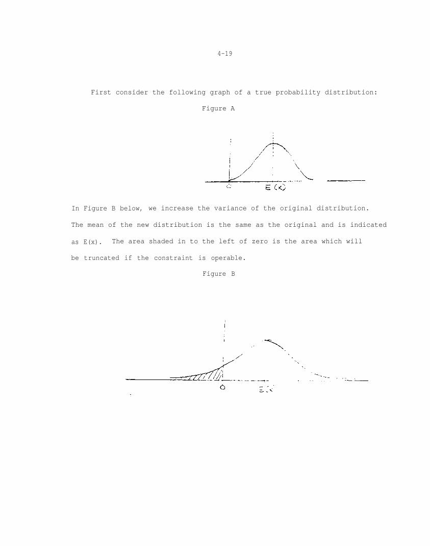
First consider the following graph of a true probability distribution:

Figure A

In Figure B below, we increase the variance of the original distribution.

The mean of the new distribution is the same as the original and is indicated

as E(x). The area shaded in to the left of zero is the area which will

be truncated if the constraint is operable.

Figure B

4-20

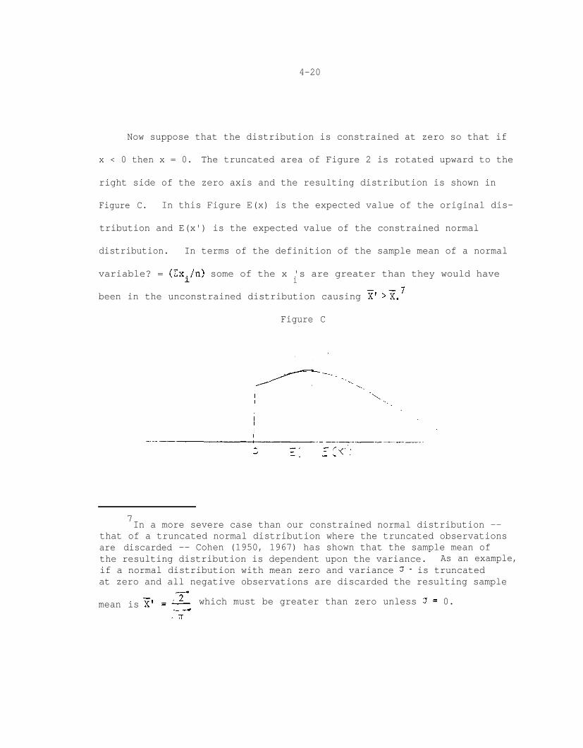
Now suppose that the distribution is constrained at zero so that if

x < 0 then x = 0. The truncated area of Figure 2 is rotated upward to the

right side of the zero axis and the resulting distribution is shown in

Figure C. In this Figure E(x) is the expected value of the original dis-

tribution and E(x') is the expected value of the constrained normal

distribution. In terms of the definition of the sample mean of a normal

variable? = (Cxi/n> some of the x 's are greater than they would havei

been in the unconstrained distribution causing x1 >?i.'

Figure C

7In a more severe case than our constrained normal distribution --

that of a truncated normal distribution where the truncated observationsare discarded -- Cohen (1950, 1967) has shown that the sample mean ofthe resulting distribution is dependent upon the variance. As an example,if a normal distribution with mean zero and variance 3 - is truncatedat zero and all negative observations are discarded the resulting sample

mean is which must be greater than zero unless J = 0.

4-21

The Relationship Between Strategic and Hypothetical Bias

A second important aspect of hypothetical bias which is unresolved

in the literature is the nature of its relationship with strategic bias.

When statements are made that: "The hypothetical nature of such (WTP) surveys

may then, in actuality, aid in eliciting bids which are not strategically

biased" (Schulze, et al., 1980:11) the implication is that hypothetical

bias is the opposite of strategic bias. According to this logic,strategic

bias occurs because people believe the situation is "real" and cover up

their "genuine" opinions to suit their perceived interests whereas it is

the unreality of the situation which promotes hypothetical bias. We

believe it is more correct to distinguish strategic from hypothetical

bias in terms of the types of realism involved, however. Strategic bias

is promoted when the consequences of the WTP questions are perceived by

the respondent as real. Hypothetical bias, in contrast, is induced when

the market described to the respondent is not realistic enough. These two

factors may vary independently as shown in Table 4.3. Respondents may

perceive that they either will have to pay the amount they state for

(continue)

4-22

Table 4.3TYPES OF REALISM AND STRATEGIC AND

HYPOTHETIC BIAS

Perceived Consequence for Respondent

4-23

the public good or that their responses will directly influence public

policy. On the table this is described as a direct consequence and

promotes strategic bias. Alternatively this consequence may not seem

likely to them, a perception which appears to be the general rule among

respondents in WTP studies including this one. Turning to the other

dimension, hypothetic bias is minimized when the hypothetical market

is credible or plausible to respondents in that it accords sufficiently

with their understanding of how the world works and imposes realistic

(albeit hypothetical) constraints on preferences (by introducing cost,

for example). It is the absence of this market realism which promotes

hypothetical bias. Both biases are minimized, therefore, when consequence

realism is low and market realism is high (cell 2 in the Table 4.3).

Schulze, et al., in a discussion of hypothetic bias argue that

both consequence and market realism are necessary for WTP surveys (cell 1):

"The contingent valuation approach requires postulating a changein environmental attributes such that it is believable to theindividual and accurately depicts a potential change. The changemust be fully understandable to him, i.e., he must be able tounderstand most, if not all, of its ramifications. The individualalso must believe that the change might occur and that his con-tingent valuation or behavioral changes will affect both thepossibility and magnitude of change in the environmental attributeor quality. If these conditions are not fulfilled, the hypotheticalnature of contingent valuation approaches will make theirapplication utterly useless." (Schulze, et al,, 1980:14).

4-24

We agree with the first part of their statement, but not the second part.

We do not believe, as they apparently do, that consequence realism is

necessary for a credible survey. Certainly none of the WTP surveys reported

in the literature on air and water pollution have achieved it, a judgment

in which Schulze and his colleagues concur; and if they had, strategic

bias would become a genuine problem for WTP surveys. In what follows

we argue that properly designed surveys can describe situations with

sufficient realism to elicit meaningful responses and discuss the adequacy

of our questionnaire in this regard. We then propose theoretically based

regression estimations as an appropriate test for hypothetical bias.

Survey Research and Market Simulation

According to Randall, et al. (1974:135) the validity of WTP surveys

"depends on the reliability with which stated hypothetical behavior is

converted to action, should the hypothetical situation posted in the game

arise in actuality." The challenge is to create a believable and meaningful

set of questions which will simulate a market for the public good in question,

Some would argue that this is an impossible task, that survey research is

too removed from reality to be able to predict behavior. This view seems

to lie behind the remarks of Gary Fromm that "It is well known that surveys

that ask hypothetical questions rarely enjoy accurate responses"

(Fromm, :172).

4-25

In fact, as Howard Schuman and Michael Johnson (1976) show in their

major literature review of the relationship between attitudes and behavior,

most studies which measure people's attitudes and their subsequent behavior

show positive results. At the individual level, for example, those Army

trainees who say they are eager for combat are significantly more likely

to perform well in combat several months later (Stouffer, et al., 1949) and

persons who say they support open housing are far more likely (70%) to sign

an open housing petition three months later than those who expressed op-

position to open housing (22%) (Brannon, et al., 1973). One study of four

elections showed behavioral intention predicted correctly to actual vote

for 83 percent of the respondents who voted (Kelley and Mirer, 1974).

Schuman and Johnson cite numerous other examples of attitude behavior

correlations and conclude that the attitude-subsequent behavior correlations which

occur "are large enough to indicate that important causal forces are

involved" (Schuman and Johnson, 1976:199) although the variance explained

by attitudinal intention is usually fairly modest.

The most impressive demonstrations of attitude-behavior correlations

occur at the aggregate level. Modern election polls predict election

results with great accuracy. The 1980 presidential election was no

exception to this generalization because the polls which took place

immediately before the vote caught the last minute shift which brought

President Reagan to power (Ladd and Ferree, 1981). For many years the

Institute for Social Research at the University of Michigan has used

4-26

survey research to measure consumer sentiments and probe the psychology of

economic behavior. Their Index of Consumer Sentiment represents a macro

measure reflect&g the changes in attitudes and expectations of all

Americans. For the past 25 years it has declined substantially prior to

the onset of every recession and it advanced prior to the beginnings of

periods of economic recovery (Katona with Morgan, 1980). These correlations

occur despite the fact that the University of Michigan economists are

unable to predict an individual's spending or saving on the basis of changes

in his or her attitudes and expectations. They attribute this paradox to

fact that individual consumer behavior is influenced by a large number of

factors including situational, attitudinal, and physical (fatigue) which make

accurate predictions of individual behavior difficult to make. The volatility

of individual behavior is smoothed out for aggregations of people; mood,

individual differences in how people react to the particular stage in the

business cycle, individual reactions to whether or not they have recently

purchased large consumer durables and the like are averaged across the

sample (Katona with Morgan, 1980:60). This is a strong argument for the

validity of surveys (provided the questions are well worded and the sampling

is adequate) as measures of aggregate benefits.

4-27

We conclude that properly designed survey questions do have the potential to ap

proximate real situations sufficiently to elicit "responsible" responses

which can be predictive of behavior under the defined circumstances

contained in the questions (Brookshire, et al., 1979:30-31). Schuman and

Johnson analyze the design factors which improve behavioral predictions,

One of the most important is the degree of congruence between the expressed

attitude and behavior. Heberlein and Black (1976), for example, found

(continue)

4-28

attitude-behavior correlations increased from .12 to .59 for the use of lead-

free gasoline when the predictive attitudes shifted from general interest in

environmental issues to a question about the degree of personal obligation the

respondent felt to buy lead-free gasoline. In a similar vein, Brookshire, d'Arge

and Schulze cite the psychologists' Ajzen and Fishbein's well known dictum that

behavioral intention and the actual behavior "should correspond, in terms

of the action, its context, its target and its time frame" (Brookshire, et

al., 1979:25).

A second important design factor is the degree of information presented

about the consequences of an attitude, particularly its financial implications.

The more fully these consequences are specified, the more realistic the

response. In the 1960s Gallup consistently found a majority of people favored

foreign aid when they were asked: "In general, how do you feel about foreign

aid -- are you for it, or against it?" In a national survey during the

same time period, Lloyd Free and Hadley Cantril introduced the pocketbook aspect

of the issue in a question which asked whether "government spending for this

purpose (foreign aid) should be kept at least at the present level, or re-

duced, or ended altogether?" When costs were raised in this manner the

majority position shifted from favoring foreign aid to wanting it reduced orsee also Mueller, 1963).

ended (Free and Cantril,1967:72;/ A similar shift occurred in a poll conducted

in the Swedish city of Malmo. In this case a sample was asked whether they

would like the Swedish government to increase aid to less-developed nations.

Later, in the same questionnaire, the respondents were asked whether they

would like this to take place "even if taxes would be raised in proportion."

Half the supporters of increased aid vanished when the question was phrased

this way, leaving only 20 percent who were willing to pay for increased aid

(Bohm, 1979:146).

4-29

The shifts in opinion evoked by the changes in question wording

are understandable because we would expect higher demand for free goods

according to economic theory, The Swedes who favor foreign aid in the

first question consist of two types of people: 1) those who favor it in

the abstract but who are not willing to pay for it when reminded of that

contingency and 2) those who favor it in the abstract and who are also

willing to pay for it, The second question induces those in category 2)

above to relinquish their support by introducing the contingency of cost.

WTP studies go one step further, of course, and ask respondents to specify

the amount of money they personally are willing to pay, This and the fact

that many other contingencies are spelled out in the questionnaire makes

them a far more realistic measure of attitudes than ordinary survey

research items.

4-30

Context Correspondence

As we noted in Chapter 2, there are special challenges in devising

a macro WTP instrument which is sufficiently realistic to avoid hypo-

thetical bias, We made special efforts, as described in Chapter 3, to

present the market for

national water quality in terms that are understandable to the respondent

and which related as closely as possible to the way the respondent actually

contributes to the provision of water quality. We will not repeat that

discussion here, but will amplify it by discussing the degree to which our

instrument is threatened by context correspondence problems, a particular7

form of hypothetic bias.

As described by Brookshire, et al. (1979, 26ff), these problems occur

"where the initial rights and endowments as well as the terminal rights and

endowments are far removed from the actual situation." The primary

example of the context correspondence problem is the failure of questions using

the willingness to accept compensation format to elicit meaningful answers.

The notion of being "bribed" to tolerate pollution is so far out of people's

ordinary comprehension that many people apparently consider it immoral and

refuse to value the environmental good at anything less than infinity

(Randall, et al., 1974; Blank, et al., 1977: Brookshire,

and above in Chapter 1). Is is possible that the high percent of no-

plays and zero bidders we found is an indicator that our instrument suffers

from context correspondence problems?

7Brookshire, et al., say a high percentage of protest votes is an

indicator of context correspondence problems (1979:28)

4-31

On an a priori basis we do not believe this to be the case. The

initial endowment of boatable water nationally and the notion that people

are paying for water quality of this level in taxes and higher prices

seems well within people's understanding, particularly since they are

already paying for water quality in this manner (although they may not have thought

about it), Our instrument assumes a structure of rights in which fresh

water is a common property resource which can be used for various purposes,

The simulated market provides a situation in which the individual buy

improved water quality situations by paying higher taxes and prices. It

assumes that these cannot be provided free of charge. It is possible that

some people may feel that businesses should pay the costs of treating

pollution out of profits instead of passing the costs on to consumers, but

surveys suggest that a large majority of the public are aware of the fact9

that these costs do get passed on to consumers (Cambridge Reports, 1978:167).

Finally, the improved situations we propose, fishable and swimmable water,

do not appear to be so far from the initial position (boatable water nationally)

to cause problems nor to deviate dramatically from the person's previous ex-

perience and preferences. Most people will have had first hand contact with

freshwater of those quality levels.

However, when we ask people to put a dollar value on water quality

levels we are asking them to do something that is not part of their normal

8In the case of going from boatable to non-boatable the respondents were

buying the continuance of the status quo. See the more detailed discussion ofproperty rights in Chapter 1 where we specify the types of consumer surplusmeasures we employ in this study.

9Cambridge Reports in a report for the Shell Oil Company asked a national

sample: "When the government imposes new health or safety standards on anindustry which single group do you think usually pays the cost of implementingthose standards: the industry out of its profits, workers in the industrythrough lower wages, consumers through higher prices or the government usingtax money? Sixty-two percent said consumers through higher prices (CambridgeReports 1978:167) and 12 percent "the government using tax money." Only 7%

4-32

behavioral repertoire; both the valuing and the contemplation of national

water quality are novel experiences for most people, By way of contrast,

those WTP studies which ask people to place a value on certain characteristics

of a particular recreational site in terms of an entrance fee ask people

to perform a much less novel act since people are familiar with entrance

fees and regularly make decisions about whether or not they are worth the

price. Does this mean that such a study is necessarily more valid than

ours? We think not,because familiarity may present problems of its own.

When respondents are asked to express WTP amounts by the entrance fee

vehicle (e.g. Thayer, forthcoming) the amount they give may represent not what

they personally consider the benefit to be worth but what they consider

to be a "fair" entrance fee based on their experience with entrance fees, Thus,

novelty as such need not be an impediment. What matters most is whether

respondents are made sufficiently familiar with the new situation in the

interview.

Where context correspondence is present we will expect two outcomes. The

first is a greater incidence of item nonresponse for the WTP items. More people

will be unable to find the situation meaningful enough to offer WTP amounts

or in protest they will bid $0. WTP surveys test for context correspondence by

examining (and reporting) the rates of these responses. As noted earlier

we had large numbers of people who failed to give amounts or who gave $0

amounts. In our discussion of this problem below, under item nonresponse

bias, we conclude that it is probably caused by problems other than

context correspondence.

4-33

Secondly, if the situation which respondents are valuing is too removed from the

experience or interests, their answers to the WTP questions will be more whimsical

than purposeful and should vary randomly. Conversely, if the task is meaningful

to the respondent, his or her answers will be constrained by the factors

which influence decisions about such expenditures in everyday life: incomevariability.

and value. The context correspondence problem in this instance is increased/

An appropriate test for randomness of responses is the size of R2 in a regression

of WTP amount on theoretically-based constraints1;

(in our case: recreational

use of freshwater, concern about water pollution, income, etc.). We

report the results of our predictive test in Chapter 5. Our findings in

this respect are very reassuring.

INSTRUMENT BIASES

The willingness to pay literature has identified four instrument

characteristics which are potential sources of bias, These are the payment

vehicle, information, order and starting- point biases. A number of studies

have varied these dimensions systematically in an effort to see whether

or not a particular instrument bias is present. Our effort in this

regard was limited to the most innovative aspect of our instrument; the

use of the payment card to elicit the respondents WTP amount. The results

of this experiment are discussed in detail under starting point bias. The

instrument was designed to minimize the effect of each of the other

potential biases.

Starting Point Bias

In Chapter 3 we discuss why we believe starting point bias is a

serious problem for bidding game studies which use payment vehicles other

10For an excellent example, see Brookshire, et al., 1980.

4-34

than admission fees to measure people's willingness to pay for public

goods. We developed the anchored payment card as a substitute for the

opening bid on the assumption that presentation of a large menu of potential

bids would minimize any tendency on the respondent's part to acquiescece

to the interviewer's suggested bid. There is the possibility of course,

that the payment card itself might bias the WTP amounts. To examine this possibility

we manipulated the two aspects of our payment cards which seemed to present

the greatest possibility of influencing respondent WTP amounts and tested

several different versions of the payment card on comparable sub-samples.

These variations and the rationale behind them are as follows:

1. The payment card is anchored with estimates for non-environmental

goods. We varied the number of goods presented from four in11

versions A and C to five in Version B. The extra good in Version B

was police and fire protection, The amount which we estimated

households spent on this good ($98, $125, $312 and $626 for the12

four income levels ) was such that it placed police and fire

protection on the payment card at a place where we guessed people

might value water quality. Except for the addition of the fifth

11In this discussion we will only consider versions A, B, C, of our

instrument. Version D was significantly different and our findings forthis version will be described elsewhere. See Chapter 3 for a descriptionof the research instrument and Appendix I for the complete wording ofall the questions.

12See Appendix III for the procedures used to derive the public good

expenditures and Appendix I for all the payment cards used in the study.

4-35

public good, the payment cards for Version B are identical

to those for Version A. If the number or placement of the

anchors affects the starting point we would expect the mean

WTP amounts for B to differ from the amounts for the other

versions.

2. In order to see whether people keyed their water benefit amounts

to the amounts shown on their card for the other public goods,

Version C displayed the same four public goods as Version A,

but each amount was increased by 25 percent. If the dollar

level of the anchor or benchmark goods determines the WTP

amounts for water quality we would expect higher mean amounts

for Version C than for Version A.

Table 4.4 summarizes the sample design for our tests of starting point bias.

We used t tests to test for the hypotheses:

Test I

Test II

Where A, B, C refers to versions A, B, C.

Table 4.44-36

STUDY DESIGN FOR EPA WATER POLLUTION BENEFITS STUDYAND NUMBER OF CASES (IN PARENTHESIS)

Versions

Scale cards with theestimated levels ofpayment for space,

A highways, publiceducation and defensefor each of the fourincome categories.

(431)*

Scale cards withcorrect payment levels

B for the four publicgoods used for A pluspolice and fire

(380)

Scale cards with samefour public goods usedfor A but the payment

C levels listed are 25%higher than those usedfor Version A

(410)

Same as A plus theD estimated amount for

water pollution control

(355)

Family Income Levels

I $9,999 or less(117)

II $10,000 to 14,999(58)

III $15,000 to 24,999(112)

Water Quality Levels

Amount willing to pay for:D Okay for boating (2.5

on 10 step ladder)

C Game fish like bass canlive in it (5.0)

B Safe for swimming (7.0)

IV $25,000 and above ornot sure/refused

(92)

Same as A Same as A

I (170)II (66)

III (98)IV (62)

Same as A

I (116)II (58)

III (126)IV (74)

Same as A

I (82)II (78)

III (103)IV (70)

Same as A

Asked whether willing topay the specific amountfor level C

If not willing to pay, askedhow much willing to keeplevel at D

If willing to pay for C,asked how much willing topay for B

"The total number of cases for each version exceeds the sum of the numberof cases ascribed to each income level for that version owing to the absenceof income data for some respondents.

4-37

The results of these tests for each income by water quality level

category are given in Table 4.5. Of the 24 paired comparisons only two

are significantly different from zero (less than the number positive

findings one would expect by chance at the .05 level) and both

are in the opposite direction to that predicted if starting point bias

is present. We conclude that for I and II, the null hypothesis

is supported: there is no evidence of starting point bias.

A second test of starting point bias was conducted using regression

analysis. We made dummy variables for each of the three versions. We

then estimated two sets of equations for pairs of versions. The first used

one of the dummy variables as the sole predictor variable, the second

is identical to the first except that we added the set of predictor variables

which are the best predictors of the WTP amounts. If Ho in Test II is incorrect,

the dummy variables for the versions should enter the equations significantly

(as measured by the t values). Table 4.6 presents the results of these

estimations. None of the version dummy variables are significant, confirming

our finding above that our instrument does not suffer from starting point

bias.

On the basis of these findings, which not only show no version effect

but also reveal an impressive stability across the versions in the multi-

variate estimations, we combine the three versions into one data set for

all further analysis.

4-38

Table 4.5

Income Level

Low 1 AB

2 AB

3 AB

High 4 AB

t TESTS OF YEAXS~FORPAIRED COMPARISONS BETWEENVERSIONS A, B, C BY INCOME AND

LEVEL OF WATER QUALITY

Level of Water Quality

Boatable Fishable Swimmable

AC

AC

AC

AC

BC AB AC BC AS

BC AB AC* BC AB AC BC

BC AB AC BC AB

BC AB AC BC AB

AC BC

AC BC

AC BC

%'wo tailed test, variances between samples were compared and then thet test was computed on pooled or separate variables as appropriate.

The one tailed t-test was insignificant for every pair of A and Cfor test I since the two significant pairs of A and C (* in the table)under the two tailed t tests are in the opposite direction from thatpredicted by Hl of test I.

*Difference between the means is significantly different from 0 atthe 5% level.

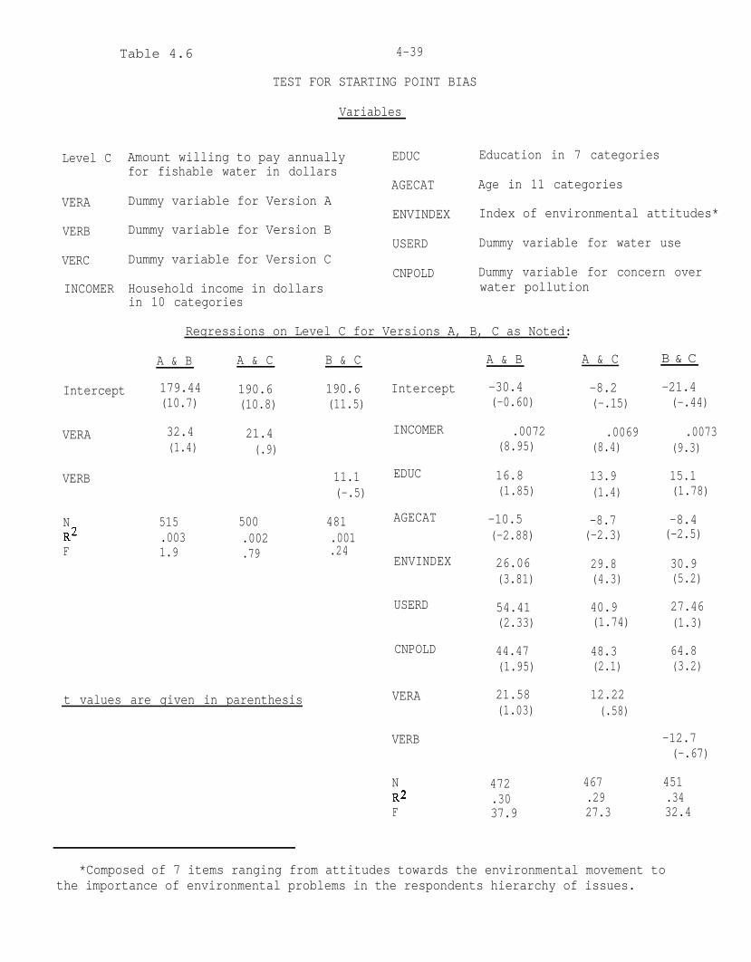
Table 4.6 4-39

Level C

VERA

VERB

VERC

INCOMER

Intercept

VERA

VERB

NR2F

TEST FOR STARTING POINT BIAS

Variables

Amount willing to pay annuallyfor fishable water in dollars

Dummy variable for Version A

Dummy variable for Version B

Dummy variable for Version C

Household income in dollarsin 10 categories

EDUC Education in 7 categories

AGECAT Age in 11 categories

ENVINDEX Index of environmental attitudes*

USERD Dummy variable for water use

CNPOLD Dummy variable for concern overwater pollution

Regressions on Level C for Versions A, B, C as Noted:

A & B A & C B & C

179.44 190.6 190.6 Intercept(10.7) (10.8) (11.5)

32.4 21.4 INCOMER(1.4) (.9)

11.1 EDUC

(-.5)

515.0031.9

500.002.79

t values are given in parenthesis VERA

481 AGECAT

.001

.24ENVINDEX

USERD

CNPOLD

VERB

N 472 467 451R2 .30 .29 .34F 37.9 27.3 32.4

A & B

-30.4(-0.60)

.0072(8.95)

16.8(1.85)

-10.5(-2.88)

26.06(3.81)

54.41(2.33)

44.47(1.95)

21.58(1.03)

A & C

-8.2(-.15)

.0069(8.4)

13.9(1.4)

-8.7(-2.3)

29.8(4.3)

40.9(1.74)

48.3(2.1)

12.22(.58)

B & C

-21.4(-.44)

.0073(9.3)

15.1(1.78)

-8.4(-2.5)

30.9(5.2)

27.46(1.3)

64.8(3.2)

-12.7(-.67)

*Composed of 7 items ranging from attitudes towards the environmental movement tothe importance of environmental problems in the respondents hierarchy of issues.

4-40

Payment Vehicle Bias

In Chapter 3 we describe why we chose annual household

payment in higher prices and taxes for our payment vehicle. There we

argue: 1) that our vehicle realistically accords with the actual form of

payment for water quality and 2) that it is familiar to respondents yet

lacks the drawbacks posed by some familiar vehicles such as entrance fees

which may limit WTP responses to an accustomed payment range rather

than to a true WTP amount. A further criteria for payment vehicles imposed

by economic theory is that they should offer respondents the widest possible

latitude of potential substitution across current commodities (Schulze,

et al., 1980:12). We believe our vehicle combines believability with the

widest latitude for substitution, two characteristics which often must be

traded off in WTP surveys (Brookshire, et al., 1979:23-4). In the ad-

ministration of the survey we encountered no problems with the vehicle.

If the vehicle suffers from any bias it is likely to be downward owing to

the current national concern over taxes and prices.

Information Bias

Information bias occurs when the wording of the instrument affects

values elicited in ways unintended by the researcher. The result is the

introduction of contingencies other than those contained in the formal

hypothetical situation. Because the opportunities for information bias

in questions are legion, the evaluation of a WTP study must

the

include a review of the wording of the entire instrument and an examination

of the quesiton. In Chapter 3 we introduce and describe the questions we

4-41

used in this study. Needless to say, we attempted to word the instrument

in such a way that by spelling out the tradeoffs, the cost, the fact that

they are already paying for public goods, etc. the respondents were presented

with a credible hypothetical market for water value. We endeavored to word

the instrument in as neutral a manner as possible so that neither the

costs nor the benefits of water quality were emphasized at the expense of

the other. Readers can judge the success of our efforts for themselves

by consulting Appendix I which contains the entire instrument in the form

it was given to the interviewers.

Order Bias

Order bias is closely related to information bias. Some information

may influence people's responses in an unwelcome manner simply because of

its location in the questionnaire. The little research that has been done

on order effects suggests that this is not an important source of bias

in surveys (Alwin, 1977:141), but good survey practice dictates that sensi-

tive or potentially biasing items should be located later in a questionnaire,

otherwise the sensitive items might lead respondents to prematurely

terminate the interview and the biasing items might affect the answers to

questions which are sensitive to that type of bias. In WTP surveys it is

important to avoid preceding the WTP items with questions which emphasize

the benefits of the good being valued at the expense of the cost or vice

versa. Rowe, et al. (1979:6) specifically cite the possible influences of

early environmental attitude questions in this regard.

4-42

The RFF water benefits was preceded by a half hour (or more) interview

on environmental and energy issues. The questionnaire for this study is

contained-in Appendix IV. What bias, if any might result from the

respondent being subjected to a searching interview about environmental

protection, environmental values, risk, energy source preferences, and

government action on these matters? Yore particularly, might these

questions stimulate a greater value for environmental quality than would

otherwise have been the case and bias the WTP amount upwards? We think

this is unlikely for the following reasons:

1. The earlier questions were realistic and balanced because they

measured environmental values in the context of the tradeoffs

associated with obtaining better environmental quality. They

a) forced people to rank order environmental goals with other

goals (Qs. 1-10), b) elicited people's views about economic and

energy problems (Qs. 11a, b, f; 21a, f; 26; 40-46) and

c) used questions whenever possible which described the tradeoffs

entailed in minimizing risk or protecting the environment

(e.g., Qs. 31, 34-36, 39, 53c).

2. A contributing factor to the realism of the RFF environmental

survey is the unique historical context of the survey. Most

of the interviewing occurred in late January and early February

1980, a time when the Iranian hostage crisis and the Russian

invasion of Afghanistan were dominating the news. These concerns,

added to the great concern expressed by our respondents about

4-43

inflation and higher prices, suggest the historical context did

not bias the respondents towards taking an environmentally

oriented position. If anything, the opposite is likely to be

the case.

3. It is possible to compare the degree of environmental support

revealed in the RFF questionnaire with the findings of a commercial

phone survey (Opinion Research Corporation, 1980) which took

place two months after most of the RFF interviewing and which

repeated several key questions word for word. The commercial

survey found even stronger support for environmental values than

did the RFF survey. This suggests that the format of the RFF

survey did not bias people towards viewing the environment with

special favor, but rather it seems to have led people to evaluate

the issues with greater realism.

In our judgment the earlier environmental/energy questions add to

the validity of the WTP study by requiring the respondents to consider a

wide range of environmental issues and their tradeoffs prior to evaluating

the worth of water quality. It is possible, however, that the length of

the first portion of the survey may have induced respondent and interviewer

fatigue. If we had used the bidding game format fatigue, if present, might

have biased the WTP results upwards by tempting respondents to acquiesce

to the starting point more often than would otherwise have been the case.

(or downwards by making their willingness to pay bid lower). Since the payment

card technique minimizes starting point bias, we have no reason to believe that

fatigue biased our results upwards in this manner. On the contrary, fatigue

may be a cause of the large number of zero amounts and no answers which

we experienced.

4-44

SAMPLING BIASES

There is a set of potential biases associated with the methodology

of survey research which have received less emphasis in the WTP literature

than they should. An instrument may be entirely free from general and

instrument biases, but if it suffers from serious sample and non-response

problems its findings cannot be generalized reliably to a larger population of

any kind and should not be used to estimate aggregate benefits. In the past some

WTP studies have made such aggregate benefit estimates on the basis of

seriously flawed samples or, worse, without even reporting the information

necesary to assess whether method biases are present or not.

Sample Bias

Scientific sampling is a process by which elements of a population

are chosen in such a way that information about those elements can be

generalized within known error ranges to the population from which the elements are

drawn. Methods of sampling are well grounded in statistical and probability

theory. There are numerous sampling techniques but the

distinguishing characteristics of a properly designed sample are that all

the units in the target population have a known, nonzero chance of being

included in the sample, and the sample design is described in sufficient13

detail to permit reasonably accurate calculation of sampling errors.

Sampling bias occurs when samples are not properly designed or reported.

=For a presentation of sampling theory and design for the non-technicalreader see Williams (1978). For a discussion of sampling for surveys seeBabbie (1973:73-130) and, especially Sudman's excellent book, Applied Sampling(1976).

4-45

The sampling method used for the RFF survey is a probability sample,

the more rigorous of the two sampling methods regularly used by commercial

survey research firms (the other being the modified probability sample).

A description of the sample, which was designed by the Roper Organization,

is presented in Appendix V. It ensures that all noninstitutionalized

persons, 18 years of age or older, who live in the lower 48 states have

a known probability of being interviewed.

There are many considerations which enter into the decision about how

many people to interview for a study,but the basic tradeoff is between

cost and accuracy, Presuming that the respondents are selected according

to sampling theory, the smaller the size of a set of respondents (which

may range from the entire sample to a sub-sample of special interest

to the analyst such as environmental activists), the larger the sampling

error. For a simple random sample, the error range at the .05 level of

confidence is 3 percent for 1,067 respondents and 7 percent for 196

(Backstrom and Hursh, 1963:33). For a sample of 50, the Opinion Research

Corporation estimates a 14% sampling error. Thus, if 25 percent of a sample

of 50 say they went boating at least once in the past two years, the true

value will lie between 11 and 39 percent, 95 percent of the time. Obviously,

if these 50 people were not chosen by proper sampling techniques the

error range is unknown,and it is impossible to say anything about what

percent of any larger population (such as the people who live in the

area where the interviewing took place) went boating in the last two years.

14For this reason, a true sample of 1500 people allows Gallup to predict

14We use "true" here to refer to a probability based sample,

4-46

a national election with great accuracy whereas a non-true sample of

100,000 is worthless for this purpose as the Literary Guild Magazine

learned to its chagrin when it predicted Landon over Franklin Roosevelt.

The RFF survey results are based on a total sample size of 1576. Much

of the analysis in this report is based on versions A, B, and C for (N=1221) for wh

we have approximately 700 valid answers to our WTP questions.

Response Rate

The results of a sample survey can be biased if "significant" number of

people selected to be part of the sample refuse to be interviewed or are

unavailable to the interviewer because of travel, sickness or work at the

time the interviewer calls. When this occurs, bias is introduced because

those not interviewed are likely to differ from those who were interviewed

in systematic ways. For example, they may be more

or less environmentally oriented. The question of what constitutes a

significant number does not have a simple answer owing to variations in

sampling design (some call for substitutions on a prespecified basis where

the person sampled is not available at the time of the interview), in

interview method (rates differ for the telephone, mail and personal interview

techniques), and in the method of calculating the response rate (since

non-responses can be due to outright refusals, to not being at home, to

terminating the interview before it is completed, etc. the way of calculating

the rate varies according to what is defined as a non-response) (Dillman,

1978:49-52).

4-47

When there are no established criteria for determining the quality

of the response rate, as is the case for most surveys which are not

conducted by professional survey research organizations, researchers should

provide sufficient information to enable the reader to evaluate the sampling15

implementation. In our case, we used a professional organization and well

established sampling procedures. The response rate for our survey is

73 percent, computed upon the number of interviews completed in households

containing people eligible for an interview. Those not interviewed included

people who refused and those who were not at home even after the interviewers

made up to three call backs to reach the person in the household designated

to be interviewed by the sampling plan. This response rate is well16

within current national sample survey practice using this methodology.

A comparison between the RFF sample and census data for age, education,

income, sex, race and region shows the RFF sample to be a close approximation

of the nation on all but education and those with the highest income (Table

4.7). Those with a less than high school education and the highest income

are somewhat under represented , a common occurrence in sample surveys

as these people are among those most likely to unavailable (the rich

travel or are less accessible; those with low educations are disproportionately

15The Colorado State researchers, for example, describe their

samples in admirable detail (Walsh, et al., 1978:19-23) and include atable which informs the reader that of 600 people originally selectedfor interview, 48 letters were returned, 231 could not be contactedby phone, 119 refused to be interviewed when contacted and 202 wereinterviewed.

16Although it is impossible to make a direct comparison, our 73 percent

may be compared to the 37% rate achieved by the Colorado State researchers(excluding the returned letters, but including in the base those the inter-viewers could not reach and those who refused?.

4-48

Table 4.7

DISTRIBUTING OF RESOURCES FOR THE FUTURE SURVEYON KEY DEMOGRAPHIC VARIABLES

Census

18 - 2425 - 3435 - 4445 - 5455 - 64

65 +

Less thanHigh schoolHigh Schoolsome college

college

Under $9,999$10 - 14,99915 - 24,999

25 +refused

RFF

16% 18%26 2215 1614 1515 1315 I.6

100 100

(age 18+) (age 25+)

25 3238 3720 1.517 16

100 100

25 2416 1728 3122 281 0- - -

1.01 100

MaleFemale

BlackWhite

New EnglandMid Atlantic

East North CentralWest North Central

South AtlanticEast South CentralWest South Central

MountainPacific

RFF Census

47% 48.7%53 5 1 .3

100 100.0

12 1287 8899 100

717179

17695

14101

617198

166

105

14101

Current Population Reports (Population characteristics: Profile or the United States: 1979)Series P-20, No. 350, U.S. Department of Commerce, Bureau of the Census, May 1980.

4-49

among the very old). Other factors may play a role here too, The 10 percent

who refused to reveal their incomes may be disproportionately well off.

The census data are not from the 1980 census (which was unavailable when the

table was constructed) which presumably will show a higher percent of peoplewith college educations than the earlier census estimates.

INTERVIEW BIASES

Item Nonresponse Bias

Respondents invariably fail to answer at least one question in an interview.

This presents a problem when the analyst wishes to generalize from a sample

to a population. Item nonresponse bias is the distortion in the estimate

of the population characteristics for a variable caused by people failing

to answer a question.

As noted earlier, this type of bias is the one which presented the

greatest problem in this study. Considering only those who answered

versions A, B, C (as has been our practice), 38 percent failed to

answer for our WTP questions and 16 percent gave a $0 amount. Strictly

speaking, the zero amounts are responses and we treated them as such,

but they bear further analysis, Since other studies have found that a

portion of the zero bids represent protest bids and not true zero

valuations, it is appropriate to treat them here under the item nonresponse

bias rubric.

Let us consider those who failed to give any amount first, In national

surveys it is common for the don't knows to range from 5-10 percent for

relatively demanding questions. This was the case with the questions which

immediately preceded the WTP items in our questionnaire.

4-50

It asked respondents for their water quality preference and received an

11 percent nonresponse rate. In comparison, the 38 percent for the WTP

items is obviously high. The three most likely explanations for this are: 1) The

general difficulty of WTP questions; 2) The peculiar difficulty of our

questions; 3) The interviewing situation for our study. We will discuss

each in turn before concluding that a combination of the first and last

of these factors is the most likely explanation for our high nonresponse

rate.

WTP surveys are very demanding of respondents and it should not be

surprising if, for comparable samples, they experience higher item non-

response rates that surveys using more common types of question. The WTP

instrument asks the respondent to attend to a description of the hypothetical

market which is necessarily detailed. It requires the respondent to value

in dollars an amenity the respondent does not customarily view in that

manner. This is an intellectually demanding task and requires a motivational

commitment which may be lacking for people for whom the public

good being valued is not particularly salient. We reviewed 13 WTP studies

to compare their item nonresponse rates on their WTP questions, Unfortunately,

less than half of these studies provide enough information about item

nonresponse to enable us to include them in the comparison. For the six

which did, the rates ranged from 1 percent for Robert Davis' pioneering study

of visits to the Maine woods (Knetsch and Davis, 1966) to 32 percent

for a sales tax vehicle used to study the value of air visibility in the

4-51

Four Corner's area (Randall, et al., 1974). In between were item non-

response rates of 2 percent (elk licenses, Brookshire, et al., 1980),

8 percent (damage from surface mining, Randall, et al., 1978), 11 percent,

17(air visibility, Brookshire, et al., 1980).

14 percent (sales tax, Walsh, et al., 1978), 20 percent (utility bill,

Brookshire, et al., 1980), and 21 percent (electric bill, Randall, et al., 1974).

These data suggest the following conclusions: 1) on the average, WTP

studies tend to have somewhat higher item nonresponse rates than regular

survey questions and yet 2) under certain conditions these rates are very

low. In Davis' case, he personally conducted all his interviews in the

Maine woods and reports very high rapport with his respondents. The elk

license payment vehicle of Brookshire, et al. (1980) is specifically and

traditionally tied to the good being valued. Because entrance fee vehicles

have the same characteristics, we would also expect them to have low item

nonresponse rates. Studies like ours which use bidding vehicles that are

less specific or traditionally tied to the good may expect higher item

nonresponse rates.

The second hypothesized cause of item nonresponse is our question

wording. While we have identified minor changes which will make the

questions clearer and more interesting to the respondents we are not aware

of serious problems in this area. In our pretest with a specially trained

interviewer only two people of 38 failed to give WTP amounts.

17Neither of the last two studies specifically report item non-

response rates. We infer these values from Randall, et al.'s, "unusable"survey figure and Brookshire, et al.'s "deletions“ for reasons not explained(presumably because the respondents gave no amount.

4-52

The interview situation is another matter. We believe this is a major

contributor to the high item nonresponse for several reasons, First, as

noted earlier, we were able to obtain a national sample at low cost because

we were able to add the benefits questionnaire to an existing survey,

Because of this, as mentioned previously, the WTP instrument was administered

after the respondents (and the interviewer) had already spent at least a

half hour on the environment/energy survey. For certain categories of

people, especially the aged and those with low levels of education, the

preceeding interview probably took longer than a half hour with cor-

respondingly greater fatigue effects. Second, because our budget was

limited, (and our purposes experimental) we did not provide the interviewers

with the kind of detailed instructions which we would provide for a full

scale benefit estimation study. These instructions would include procedures

for handling various types of respondent: queries and instructions for

encouraging reluctant players to give WTP amounts. Third, the same budget

constraints restricted the length of our WTP instrument. The addition

of several followup questions in the instrument itself which would probe

non-responses (and zero amounts) would enable us to identify respondents

who would give us WTP amounts after further explanations.

To summarize, the most likely explanation for our high item non-

response rate is a combination of the inherent difficulty of WTP questions,

and the limitations of our interview situation. Appropriate changes in

the latter, combined with a fine tuning of the questions, should reduce

the item nonresponse rate to a tolerable level, Because of the inherent

4-53

difficulty of these types of questions, it will be very difficult to

bring item nonresponse rates from 10-15 percent for WTP surveys

of the general public. Rates of this level should not unduly bias the

final estimates if weighting procedures are used to compensate for the

nonrespondents. We discuss these matters further in Chapter 6.

How will our item nonresponse rate of 39 percent bias these data?

Put another way, this question becomes: What kinds of people failed to

respond to our WTP questions? We estimated a logit regression equation

for a combination of background variables and key attitude items which

is presented in Table 4.8. Definitions for these variables are given on

Table 4.6, page 4-39 The dependent variable is a dummy with the non-

respondents set at 1 and all those who gave WTP amounts greater than zero

for fishable water at 0. (Thus we drop those who gave zero amounts from

the following analysis). The overall predictive accuracy coefficient of

.27 indicates a moderate fit. Older people, blacks and those who are

uncertain about the nation's water quality goals (0.81 SPRECHLD) were especially

likely (p. = .OO1> and those respondents low in income and education were

very likely (p. = .O1> to be among the nonrespondents. The respondent's sex

and use of water for recreation were also significantly related to the dependent

variable. This profile is consistent with the hypothesis that people for

whom the issue is less salient (SPRECHLD, RACED) and/or for whom the WTP

instrument is difficult to answer(AGECAT, EDUC, SPRECHLD) are more likely

to be among the nonrespondents to the WTP items. It is noteworthy that

environmental and water quality attitudes (ENVINDEX, CNPOLD) are not

significant in this equation.

Table 4.84-54

LOGITl REGRESSIONS RELATING BACKGROUND ANDATTITUDINAL VARIABLES TO CERTAIN TYPES OF

WILLINGNESS TO PAY RESPONSES FOR FISHABLE WATER2

Dependent variable; Dependent variable;Independent 1 = zero wtp amount; 1 = 'don't know' how muchVariables 0 = WTP amount greater willing to pay

than zero 0 = WTP amount greater than zero

Intercept

INCOMER -.0002* -.00002**

EDUC -.42*** -.23**

AGECAT .14** .09***

RACED -.95** -1.38***

SEXD -.10 .39*

USERD -1.11*** -.44*

ENVINDEX -.44*** -.08

CNPOLD

SPRECHLD3

-.23 -.15

-.96** -1.68***

N 695 783Likelihood ratio index .31 .18R2 index (D) .25 .19

Percent correctly predictedzero amounts 84%other amounts 86

Predictive accuracycoefficient .47

don't know 77%other amounts 78

.27

* p < .05 / ** p < l .01 / *** p < .001

1Xaximum likelihood estimates are computed by the Newton-Raphson method.(SAS Institute, 1980).

2For Versions A, B, and C combined.

3Dummy variable where 1 = nation should plan to achieve nationwide waterquality of fishable or better within the next five years (Q.81); 0 = all otherresponses of which "not sure" comprises two-thirds and preference for nationwidewater quality lower than fishable comprises one-twelfth.

4-55

From what we know about the willingness to pay for water quality

of other respondents, the bias given our estimates by the high item non-

response rate is upwards. The older, less educated and lower income

people who expressed WTP amounts gave lower amounts, other things being

equal, than their peers, and we would expect the addition of a significant

number of the nonrespondents to those giving WTP amounts to lower the mean

WTP value for water quality.

Turning now to the zero amounts, sixteen percent of our sample gave

WTP amounts of $0 for fishable water. It is very difficult to compare

this with the experience of other WTP studies since only four of the 13

studies reviewed report the total percent of $0 bids. For these studies

the zero amounts varied as follows: 1 percent, Maine Woods (Knetsch

and Davis, 1966); 2 percent for sales tax vehicle and 26 percent for

utility bill option, water quality in the South Platte River Basin

(Walsh, et al., 1978); 6 percent for non-reservation residents, air

pollution visibility in Four Corner's area (Randall, et al., 1974); and

7-32 percent, depending on WTP version, decreased risk from nuclear plant

accidents (Mulligan, 1978). Our level of zero amounts is somewhere

in the middle of this distribution, but we do not regard this level of

zero amounts as acceptable, especially since we already have a high non-

response rate for the WTP questions.

4-56

their true value in any future use of our instrument.

The factors discussed above for nonresponse are also the likely

cause of the zero amounts. Question wording probably played a much

larger role in stimulating the zero responses, however. Endeavoring

to legitimate low values for respondents who might have been hesitant

to express their "true" feelings about water quality, we ended the first

WTP question in the series by saying: "If it is not worth anything to you,

please do not hesitate to say so." In retrospect we believe this was

too strong a statement which unnecesarily promoted zero responses by

some who probably have valued water at greater than zero but who were

reluctant to undertake the mental effort necessary to arrive at that value.

We will substitute another type of encouragement to respondents to give

We estimated a logit regression for

a dummy variable with zero WTP set at 1 and those who gave amounts greater

than zero at 0. This regression is also reported in Table 4.7. This

estimation has superior predictive power to the parallel one for

nonrespondents (predictive accuracy coefficient of .47). Comparing the

two equations we find recreational use and environmentalism play a

greater role in predicting the zero bidders, who tend to use water less

and are weaker in their support for environmentalism. These findings are consiste

with the hypothesis that zero bids do represent low (if not zero) value

for water quality. However, the importance of age, also significant

in the equation at the .001 level, and the role of race and education (.01),

4-57

parallel their place in the nonresponse equation and suggests that zero

bids may also be partially due to people protesting the WTP format or

expressing an unwillingness to answer the question.

The bias introduced by the large number of zero bidders is to make

our estimates lower than they would be if we had fewer zero bidders.

From the findings of other WTP studies which have asked their zero

bidders why they bid zero (Rowe, et al., 1979a; Thayer forthcoming,

Brookshire, et al., 1980; Brookshire, et al., 1976) it seems very likely

that some of our zero bidders are probably protesting the instrument

rather than really valuing water quality at $0. An indeterminate

number of the remaining zero bidders, while not protesting, nevertheless

probably value water quality at least somewhat higher than $0 and could

be induced to bid higher by the changes described above.

(continue)

4-58

Interview Procedure and Interviewer Biases

Two other interview method biases remain to be discussed. The

interview procedure-bias refers to bias introduced by the manner of conducting

the interview. Interviewing takes place by either personal interview,

telephone or mail. The differences involved in choosing

between these methods including cost, return rate, ease of asking sensitive

questions, and ease of asking complex questions. Although it is the most

expensive method, the personal interview method is superior to the other

methods on all dimensions (Dillman, 1978:74-76; on social desirability

see Bradburn and Sudman, 1979:8). The personal interview method is especially

preferable for WTP surveys because it permits the researcher to use visual

displays such as our ladder and payment cards and it is the most successful

of these methods when the questions are potentially tedious and boring

(Dillman, 1978:75). The only viable alternative would be the mail survey,

a method used only twice in a WTP study to our knowledge (Bishop and Heberlein,

1980; Fish and Wildlife Service, 1975) as the need to create the hypothetical

market in sufficient detail is too wordy for phone interviews.

Unlike the mail surveys, personal interview surveys are open

to potential interviewer bias. This type of bias consists of differential

effects introduced by the individual interviewers. In a bidding game,

for example, some interviewers may be more skillful in inducing respondents

to increase their bids above the starting point more than others. If a

study uses relatively few interviewers who conduct 25 interviews or more,

it is possible to test for interviewer effects by holding the respondents'

4-59

personal characteristics (such as income) constant and comparing the mean

WTP amounts to see if they differ significantly. Because Roper used

100 interviewers scattered across the country to conduct our interviews,

the number of interviews per interviewer is too few to conduct this type

of test. With that many interviewers we would expect individual inter-

viewer effects, if there are any, to average out. There is always the

possibility that the interviewer training may induce all the interviewers

in a project to obtain higher bids than interviewers trained by someone

else might with the same questionnaire, but there is no easy way to test

for this other than to conduct elaborate methodological experiments.

One advantage of our payment card technique is that it minimizes the

potential interviewer effect on the WTP amount as compared with the

bidding game method.