chapter 3 : sampling variability and confidence...
TRANSCRIPT

This chapter is from Introduction to Statistics for Community College Students, 1st Edition, by Matt Teachout, College of the Canyons, Santa Clarita, CA, USA, and is licensed
under a “CC-By” Creative Commons Attribution 4.0 International license – 10/1/18
Chapter 3: Sampling Variability and Confidence Intervals Vocabulary
Population: The collection of all people or objects to be studied.
Census: Collecting data from everyone in a population.
Sample: Collecting data from a small subgroup of the population.
Statistic: A number calculated from sample data in order to understand the characteristics of the data. For example, a sample mean average, a sample standard deviation, or a sample percentage.
Parameter: A number that describes the characteristics of a population like a population mean or a population percentage. Can be calculated from an unbiased census, but is often just a guess about the population.
Sampling Distribution: Take many random samples from a population, calculate a sample statistic like a mean or percent from each sample and graph all of the sample statistics on the same graph. The center of the sampling distribution is a good estimate of the population parameter.
Sampling Variability: Random samples values and sample statistics are usually different than each other and usually different than the population parameter.
Point Estimate: When someone takes a sample statistic and then claims that it is the population parameter.
Margin of Error: Total distance that a sample statistic might be from the population parameter. For normal sampling distributions and a 95% confidence interval, the margin of error is approximately twice as large as the standard error.
Standard Error: The standard deviation of a sampling distribution. The distance that typical sample statistics are from the center of the sampling distribution. Since the center of the sampling distributions is usually close to the population parameter, the standard error tells us how far typical sample statistics are from the population parameter.
Confidence Interval: Two numbers that we think a population parameter is in between. Can be calculated by either a bootstrap distribution or by adding and subtracting the sample statistic and the margin of error.
95% Confident: 95% of confidence intervals contain the population value and 5% of confidence intervals do not contain the population value.
90% Confident: 90% of confidence intervals contain the population value and 10% of confidence intervals do not contain the population value.
99% Confident: 99% of confidence intervals contain the population value and 1% of confidence intervals do not contain the population value.
Bootstrapping: Taking many random samples values from one original real random sample with replacement.
Bootstrap Sample: A simulated sample created by taking many random samples values from one original real random sample with replacement.
Bootstrap Statistic: A statistic calculated from a bootstrap sample.

This chapter is from Introduction to Statistics for Community College Students, 1st Edition, by Matt Teachout, College of the Canyons, Santa Clarita, CA, USA, and is licensed
under a “CC-By” Creative Commons Attribution 4.0 International license – 10/1/18
Bootstrap Distribution: Putting many bootstrap statistics on the same graph in order to simulate the sampling variability in a population, calculate standard error, and create a confidence interval. The center of the bootstrap distribution is the original real sample statistic.
Introduction: The goal of learning Statistics or Data Science is to be able to analyze data to learn about populations in the world around us. The best way to understand a population is collect and analyze unbiased data from that population, namely a census. The trouble is we rarely have an unbiased census. It is sometimes impossible to collect data from everyone in a population. We have to rely on samples, small subgroups of the population. The next few chapters deal with the subject of using samples to understand populations. This is sometimes called “inferential statistics”. We will start by trying to distinguishing between population parameters from sample statistics.
Section 3A – Population Parameters and Sample Statistics Vocabulary
Population: The collection of all people or objects to be studied.
Census: Collecting data from everyone in a population.
Sample: Collecting data from a small subgroup of the population.
Bias: When data does not represent the population.
The goal of collecting and analyzing data is to understand the world around us. To this end, our goal is understand populations. The population is all of the people or objects you plan to study. A population can be large (like all people l iving in Brazil) or small (l ike all students in a particular statistics class). It goes without saying that the larger the population the more difficult it is to understand.
The best data for representing populations is an unbiased census. A census is an attempt to collect data from everyone in a population. A census is easier if we have a small population l ike the people in a particular statistics class. The advantage of collecting an unbiased census is that we can calculate population values (parameters) directly with reasonable certainty. Governments may sometimes attempt to do a census and collect data on all of the people l iving in a particular country. It should be noted that though they attempt to get data on everyone, they rarely succeed. There will always be some people fall through the cracks and are not represented in the census. An unbiased census of a large population still represents a high percentage of the people, so is generally better than a small sample of people.
A data scientist rarely has the ability to collect a census unless the population is relatively small. People that work in statistics and data science usually rely on collecting samples. Remember a sample is a small subgroup of the population. It is usually less than 10% of the population and is often significantly less than 10%. If the sample is unbiased, we then try to analyze the sample data and make guesses as to what is happening at the population level. Therefore, a data scientist or statistician needs to be able to use sample values (statistics) to figure out approximate population value (parameters).
Statistic: A number calculated from sample data in order to understand the characteristics of the data.
Parameter: A population value. It can be calculated from an unbiased census, but is often just a guess about what someone thinks the population value might be.

This chapter is from Introduction to Statistics for Community College Students, 1st Edition, by Matt Teachout, College of the Canyons, Santa Clarita, CA, USA, and is licensed
under a “CC-By” Creative Commons Attribution 4.0 International license – 10/1/18
It is very important to note that statistics and parameters are not the same thing. A statistic calculated from 250 people in a sample will often be very different from the actual population parameter from millions of people. The question that is important to ask is how far off is the sample statistic from the population parameter? That is sometimes called “margin of error” and is a key topic in this chapter.
Common Statistics
x̅ : (“x-bar”) Sample mean average
s : Sample standard deviation (typical distance from the sample mean)
𝑠𝑠2: Sample variance (sample standard deviation squared)
p̂ : (“p-hat”) Sample proportion (sample percentage)
n : Sample size or frequency (number of people or objects in the sample)
r : Sample correlation coefficient (measures quantitative relationships between samples)
𝑏𝑏1 : Sample slope (The slope of a regression l ine calculated from sample data.)
𝑏𝑏0 : Sample Y-intercept (The Y-intercept of a regression line calculated from sample data.)
Common Parameters
µ : (“mu”) Population mean average
σ : (“sigma”) Population standard deviation (typical distance from the population mean)
𝜎𝜎2: Population variance (population standard deviation squared)
π: (“pi”) Population proportion (population percentage) (Some people use “p” for population proportion.)
N : Population size or frequency (number of people or objects in the population)
ρ : (“rho”) Population correlation coefficient (measures quantitative relationships between populations. Note this is not a “p”. It is the greek letter “rho”.)
𝛽𝛽1 : Population slope (The slope of the population regression l ine. Used when studying quantitative relationships between populations.)
𝛽𝛽0 : Population Y-intercept (The Y-intercept of the population regression line. Used when studying quantitative relationships between populations.)
Let’s look at some examples of using statistics and parameters. It is important to be able to identify if a number used is a statistic or a parameter and what letter we might use in the computer program.

This chapter is from Introduction to Statistics for Community College Students, 1st Edition, by Matt Teachout, College of the Canyons, Santa Clarita, CA, USA, and is licensed
under a “CC-By” Creative Commons Attribution 4.0 International license – 10/1/18
Example
“We think the mean average ACT score for all high school students is about 22. The mean average ACT score for a random sample of 85 high school students was 21.493”
µ = 22 (parameter) n = 85 (statistic) x̅ = 21.493 (statistic)
Example
“A random sample showed that 13.2% of adults were infected, but this indicates that the population percentage could be 17%”. (Note: Computer programs often require you to convert the percentages into decimal proportions.)
p̂ = 0.132 (statistic) π = 0.17 (parameter)
Example
The standard deviation for the heights of all women is thought to be about 2.5 inches. A random sample of women heights had a standard deviation of 2.618 inches.
σ = 2.5 (parameter) s = 2.618 (statistic)
Example
“Sample data indicated that the correlation coefficient was 0.239 and the slope was 47.3 dollars per pound. Let’s compare these to the population claims that the correlation coefficient is zero and the slope is about 50 dollars per pound.”
r = 0.239 (statistic) 𝑏𝑏1 = 47.3 (statistic) ρ = 0 (parameter) 𝛽𝛽1 = 50 (statistic)
Problem Set Section 3A Directions: Determine if the numbers in the following clips from magazines and newspapers are describing a population parameter or a sample statistic. In each case give the symbol we would use for the parameter or statistic (N , n , π , p̂ , µ , x ̅, σ , s , 𝜎𝜎2, 𝑠𝑠2, ρ , r , 𝛽𝛽1 , 𝑏𝑏1)
1. “Our study found that of the 200 people tested in the sample, only 3% showed side effects to the medication.”
2. “It has been speculated for years that the mean average height of all men is 69.2 inches, but our sample data disagrees with this. Our sample mean average was 69.5 inches.”

This chapter is from Introduction to Statistics for Community College Students, 1st Edition, by Matt Teachout, College of the Canyons, Santa Clarita, CA, USA, and is licensed
under a “CC-By” Creative Commons Attribution 4.0 International license – 10/1/18
3. “The standard deviation for all humans is about 1.8 degrees Fahrenheit. A random sample of 52 people found a standard deviation of 1.739 degrees Fahrenheit”.
4. “We tested a sample of 300 incoming college freshman and found that their mean average IQ was 101.9 with a standard deviation of 14.8”.
5. “The mean average human body temperature has long been thought to be 98.6 degrees Fahrenheit, but our sample of 63 randomly selected adults had a mean average was 98.08”.
6. “The mean average number of units that students take per semester is about 12, but when we took a random sample of 160 college students found that the mean average was 12.37 units.”
7. “A public opinion poll showed that 47.2% of voters would vote for the candidate, but when the votes or entire population were counted we found that only 41.3% voted for the candidate.”
8. “According to the California Department of Finance, the Los Angeles county population as of January 2015 was approximately 10,136,559 people.”
9. “We want to check and see if the population correlation coefficient could be zero. The sample correlation coefficient was 0.338.”
10. “Many experts think that the population slope for weight gain in these type of bears is about 3 pounds per month, but the sample slope from 54 bears was 2.7055 pounds per month.”
11. “A random sample of 40 men found that the sample variance for systolic blood pressure was 109.474, but this indicates that the population variance could be as high as 173.”
Section 3B – Sampling Variability and Sampling Distributions If you wanted to study baseball players, would you only study one baseball player? If you wanted to study bears, would you only study one bear? The answer of course is no. When studying a topic like bears or baseball players, we should look at many different bears, many different baseball players. The problem with studying samples is that we usually only collect one sample at a time. We cannot learn about the behavior and variability in samples if we only look at one sample. We need to look at hundreds or even thousands of samples.
Sampling Distributions
Suppose we take many, many random samples from a population. From each random sample we calculate a statistic l ike the sample mean average. If we put all of those sample means on the same graph, we have created a “sampling distribution”. Sampling distributions are one of the best ways to understand random samples and sampling variability.
In the real world, a data scientist has only one random sample and may have no idea what a population parameter is. In this example, we will be creating a sampling distribution by take random samples from a census. We will assume the census is unbiased. With an unbiased census, we will know what the population parameter is. That way we can compare our sample statistics to the parameter and study the variability.
Example: Work Hours per Week for working COC Statistics Students (Fall 2015 semester)
We will start by looking at a census of the work hours of all of the working Math 140 students in the Fall 2015 semester. It should be noted that we are only studying the statistics students that said they work in addition to

This chapter is from Introduction to Statistics for Community College Students, 1st Edition, by Matt Teachout, College of the Canyons, Santa Clarita, CA, USA, and is licensed
under a “CC-By” Creative Commons Attribution 4.0 International license – 10/1/18
going to school. We removed all of the students that work zero hours. We will take a lot of random samples of size 50 from this census data and create a sampling distribution for various statistics.
Census Data (Work Hours per Week for working COC Stat Students Fall 2015)
We see that the census data is skewed right with a population mean average of 27.283 hours per week, a population standard deviation of 12.969 hours per week, and a population median of 25 hours per week. We will assume that the census was unbiased and these are parameters.
Population mean = 27.283 hours per week Population standard deviation = 12.969 hours per week Population median = 25 hours per week
We learned in chapter 1 that random samples tend to minimize sampling bias, so are better representations of the populations than other samples that are not random. Does this mean that random samples are perfect representations of the population? Let’s see.
Sample 1: Here is one random sample of 50 statistics students from the work hours census data.
This chapter is from Introduction to Statistics for Community College Students, 1st Edition, by Matt Teachout, College of the Canyons, Santa Clarita, CA, USA, and is licensed
under a “CC-By” Creative Commons Attribution 4.0 International license – 10/1/18
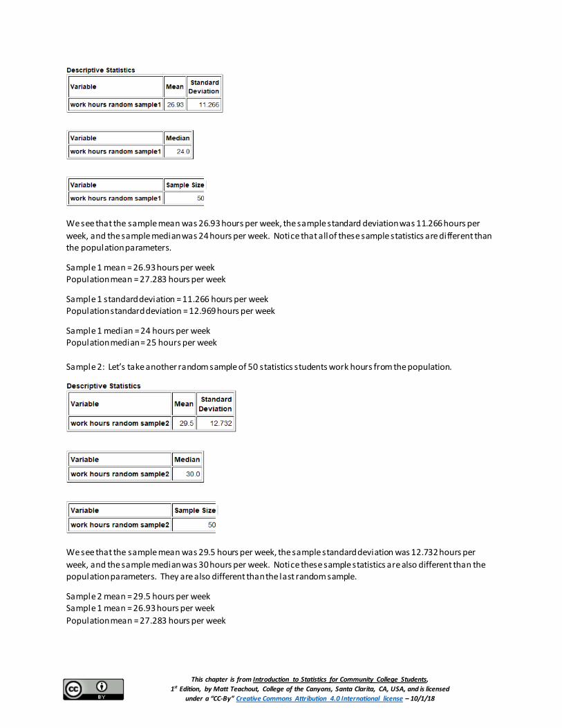
We see that the sample mean was 26.93 hours per week, the sample standard deviation was 11.266 hours per week, and the sample median was 24 hours per week. Notice that all of these sample statistics are different than the population parameters.
Sample 1 mean = 26.93 hours per week Population mean = 27.283 hours per week
Sample 1 standard deviation = 11.266 hours per week Population standard deviation = 12.969 hours per week
Sample 1 median = 24 hours per week Population median = 25 hours per week Sample 2: Let’s take another random sample of 50 statistics students work hours from the population.
We see that the sample mean was 29.5 hours per week, the sample standard deviation was 12.732 hours per week, and the sample median was 30 hours per week. Notice these sample statistics are also different than the population parameters. They are also different than the last random sample.
Sample 2 mean = 29.5 hours per week Sample 1 mean = 26.93 hours per week Population mean = 27.283 hours per week

This chapter is from Introduction to Statistics for Community College Students, 1st Edition, by Matt Teachout, College of the Canyons, Santa Clarita, CA, USA, and is licensed
under a “CC-By” Creative Commons Attribution 4.0 International license – 10/1/18
Sample 2 standard deviation = 12.732 hours per week Sample 1 standard deviation = 11.266 hours per week Population standard deviation = 12.969 hours per week
Sample 2 median = 30 hours per week Sample 1 median = 24 hours per week Population median = 25 hours per week
These examples show us that random sample statistics will usually be different than the population parameters. Random sample statistics will also be different than each other. Every time we take another random sample from the same population we will get different values. This is the principle of “sampling variability” and is a major roadblock on the quest to estimating population parameters.
Sampling Variability: Random samples values and sample statistics are usually different than each other and usually different than the population parameter.
Let’s continue taking random samples from the population of working statistics students in Fall 2015. Every time we take a random sample we keep getting different values and different statistics. Hardly any of the samples are close to the population parameter. In this example, we will focus on the mean. Remember the population mean average was 27.283 hours per week. No matter how many random samples we take, the sample means are usually different than the population mean of 27.283 hours per week. Every sample has a “margin of error”.
Margin of Error: How far off a sample statistic can be from the population parameter.
In the first random sample, the sample mean was 26.93 hours per week. So the sample mean of 26.93 hours per week was 0.353 hours lower than the population mean of 27.283 hours per week. This is the margin of error.
In the second random sample, the sample mean was 29.5 hours per week. So the sample mean of 29.5 hours per week was 2.217 hours higher than the population mean of 27.283 hours per week. Again, that is the margin of error for that sample.
What does this tell us?
The principle of sampling variability tells us that sample statistics will usually be off from the population parameter. In other words, almost all samples have a margin of error. Sometimes random samples are closer to the population parameter like sample 1 and sometimes the random samples are farther away l ike sample 2.
Important Note: If you know the population parameter, then it is relatively easy to calculate the margin of error (sample statistic – population parameter). Most of the time, we are working with sample data, so have no idea what the population parameter is. In that case, it is much more difficult to figure out the potential margin of error. Formulas were developed in order to estimate what the margin of error could be.
Point Estimates
People are usually very interested to know population values. However, we rarely ever know the population parameter. In the real world, we usually only have one random sample. Sometimes, a person will simply tell you that the sample statistic is the population parameter. This is called a “point estimate” and tends to create a lot of confusion for people.
Point Estimate: When someone takes a sample statistic and then claims that it is the population parameter.
In an article published by a health website, the author states that the population average weight of all men in America is 196 pounds. As with most articles, this is a guess about the population average and is not the actual

This chapter is from Introduction to Statistics for Community College Students, 1st Edition, by Matt Teachout, College of the Canyons, Santa Clarita, CA, USA, and is licensed
under a “CC-By” Creative Commons Attribution 4.0 International license – 10/1/18
population average weight of men. We call this a “point estimate”. Someone took a sample of men and weighed them. We do not know the sample size or if the sample was even random. They calculated the sample average and found it to be 196 pounds. Since no one really knows the population average weight of all men in the U.S., the author simply tells us the sample average is the population average.
Think about the principle of sampling variability that we just learned. We said that a sample statistic usually has a margin of error is off from the population parameter. Yet people reading the article believe that the population average weight of all men in the U.S. is exactly 196 pounds.
Population parameters may be calculated if we had an unbiased census, but remember that is rare. (Certainly we do not have an unbiased census of the weights of all men in the U.S.) Usually, we have one random sample. When reading an article that claims to know a population parameter like a population mean or population percentage, it is important to realize that it is just a guess about the population parameter, and that guess probably came from a sample. Sample statistics can be very off from the actual population parameter.
Sampling Distributions for Sample Mean Averages
Let’s go back to the example of working COC statistics students in the Fall 2015 semester. We have seen that the population mean average is 27.283 hours per week, but the two random samples of 50 statistics students gave sample means that have both been off from that population mean.
Let’s continue to collect random samples of size 50 and calculate sample means. We collected 251 random samples and calculated 251 sample means. If we put all of the sample means on the same graph, we can create a sampling distribution.

This chapter is from Introduction to Statistics for Community College Students, 1st Edition, by Matt Teachout, College of the Canyons, Santa Clarita, CA, USA, and is licensed
under a “CC-By” Creative Commons Attribution 4.0 International license – 10/1/18
Here is the sampling distribution we created with Statcato. Each dot in the sampling distribution represents the sample mean of a random sample. We also created a histogram of the sampling distribution to better judge the shape. Notice a few things.
• We took 251 random samples and calculated 251 sample means. We see sampling variability in action. The population mean is 27.283 hours per week but sample means ranged between 22.28 hours and 32.58 hours. Random sample means are usually not the same as each other and can be very different than the population mean.
• Despite the population being skewed right, the sampling distribution for these sample means is normal. This is often referred to as the “Central Limit Theorem”.
• The center of the sampling distribution is 27.127 hours. This is not the mean of a sample. It is the mean average of all the sample means. Notice that the center of the sampling distribution is very close to the population mean of 27.283 hours.
• We also calculated the “standard error”. This is the standard deviation of the sampling distribution (or the standard deviation of all the sample statistics) and is an important measure of sampling variability. Think of it this way. The standard error tells us how far typical sample statistics are from the center of the sampling distribution. Since the center of the sampling distribution is 27.127 hours and is pretty close to the population parameter of 27.283 hours, the standard error tells us how far typical sample statistics are from the population parameter. In this case, it tells us that typical sample means are approximately within 1.916 hours of the population mean.
This chapter is from Introduction to Statistics for Community College Students, 1st Edition, by Matt Teachout, College of the Canyons, Santa Clarita, CA, USA, and is licensed
under a “CC-By” Creative Commons Attribution 4.0 International license – 10/1/18
Important Note: Don’t confuse the standard error with the margin of error. The standard error tells us how far typical sample statistics are from the population value, but not all random samples are typical. Remember we learned from the empirical rule that typical for normal data represents only the values that are within 1 standard deviation from the mean (middle 68%). Usually sample values can be up to two standard deviations from the mean (middle 95%). So early statisticians thought that the margin of error should be about twice as large as the standard error. This is still a common formula for margin of error.
Margin of Error = 2 × Standard Error
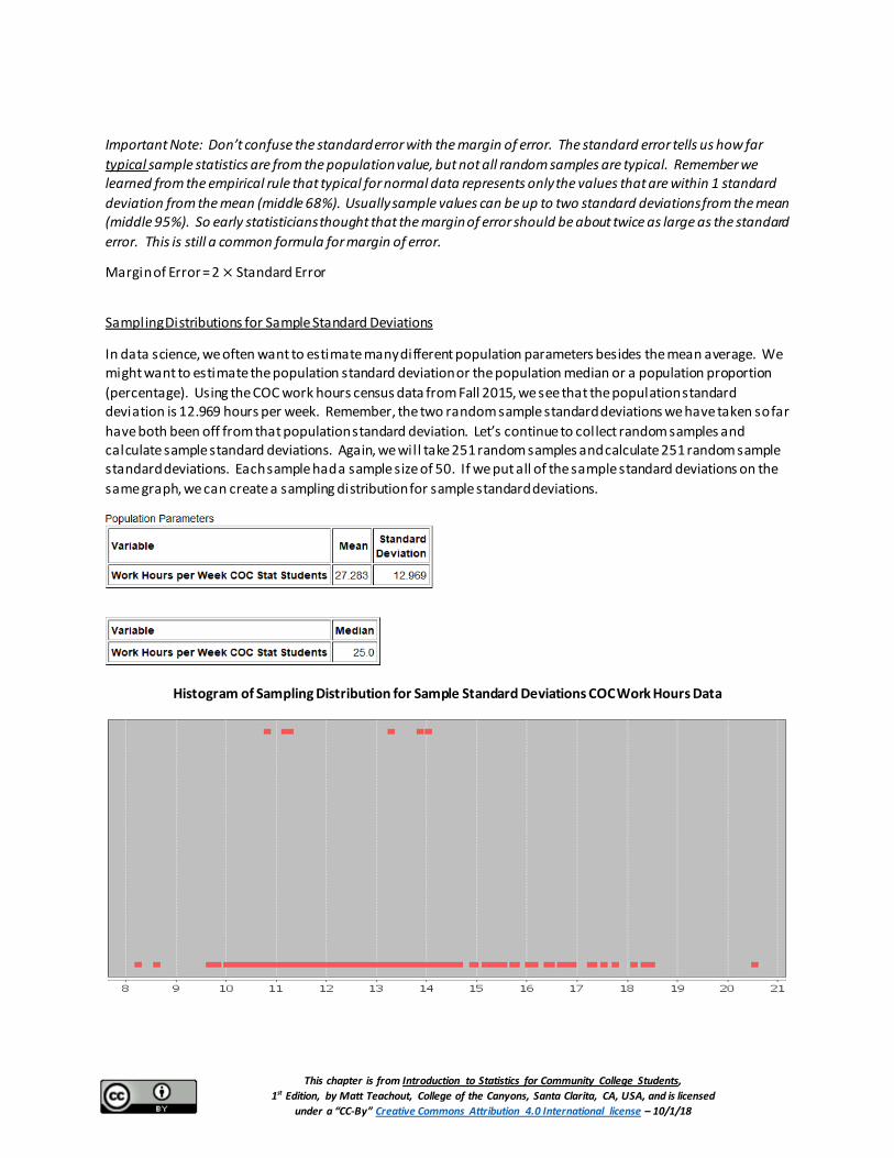
Sampling Distributions for Sample Standard Deviations
In data science, we often want to estimate many different population parameters besides the mean average. We might want to estimate the population standard deviation or the population median or a population proportion (percentage). Using the COC work hours census data from Fall 2015, we see that the population standard deviation is 12.969 hours per week. Remember, the two random sample standard deviations we have taken so far have both been off from that population standard deviation. Let’s continue to collect random samples and calculate sample standard deviations. Again, we will take 251 random samples and calculate 251 random sample standard deviations. Each sample had a sample size of 50. If we put all of the sample standard deviations on the same graph, we can create a sampling distribution for sample standard deviations.
Histogram of Sampling Distribution for Sample Standard Deviations COC Work Hours Data
This chapter is from Introduction to Statistics for Community College Students, 1st Edition, by Matt Teachout, College of the Canyons, Santa Clarita, CA, USA, and is licensed
under a “CC-By” Creative Commons Attribution 4.0 International license – 10/1/18
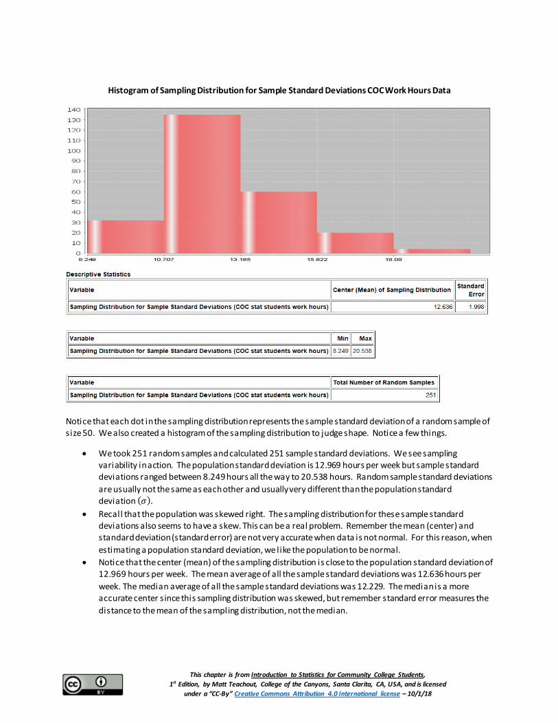
Histogram of Sampling Distribution for Sample Standard Deviations COC Work Hours Data
Notice that each dot in the sampling distribution represents the sample standard deviation of a random sample of size 50. We also created a histogram of the sampling distribution to judge shape. Notice a few things.
• We took 251 random samples and calculated 251 sample standard deviations. We see sampling variability in action. The population standard deviation is 12.969 hours per week but sample standard deviations ranged between 8.249 hours all the way to 20.538 hours. Random sample standard deviations are usually not the same as each other and usually very different than the population standard deviation (𝜎𝜎).
• Recall that the population was skewed right. The sampling distribution for these sample standard deviations also seems to have a skew. This can be a real problem. Remember the mean (center) and standard deviation (standard error) are not very accurate when data is not normal. For this reason, when estimating a population standard deviation, we like the population to be normal.
• Notice that the center (mean) of the sampling distribution is close to the population standard deviation of 12.969 hours per week. The mean average of all the sample standard deviations was 12.636 hours per week. The median average of all the sample standard deviations was 12.229. The median is a more accurate center since this sampling distribution was skewed, but remember standard error measures the distance to the mean of the sampling distribution, not the median.

This chapter is from Introduction to Statistics for Community College Students, 1st Edition, by Matt Teachout, College of the Canyons, Santa Clarita, CA, USA, and is licensed
under a “CC-By” Creative Commons Attribution 4.0 International license – 10/1/18
• The standard error was 1.998. Remember, the standard error tells us how far typical sample statistics are from the center (mean) of the sampling distribution. Since the center of the sampling distribution is pretty close to the population value, the standard error tells us how far typical sample statistics are from the population parameter. In this case, it tells us that typical sample standard deviations are within 1.998 hours of the population standard deviation. Again, the accuracy of the center (mean) and the spread (standard error) are in question because the sampling distribution did not look normal.
Sampling Distributions for Sample Median Averages
When data is skewed, we saw that the median average is usually more accurate than the mean, but how well do sample medians approximate population medians? Using the COC work hours census data from Fall 2015, we see that the population median is 25 hours per week. Remember, the two random sample medians we have taken so far have both been off from that population median. Let’s continue to collect random samples and calculate sample medians. Again, we will take 251 random samples and calculate 251 random sample medians. All of the samples had a sample size of 50. If we put all of the sample medians on the same graph, we can create a sampling distribution for sample medians.

This chapter is from Introduction to Statistics for Community College Students, 1st Edition, by Matt Teachout, College of the Canyons, Santa Clarita, CA, USA, and is licensed
under a “CC-By” Creative Commons Attribution 4.0 International license – 10/1/18
Notice that each dot in the sampling distribution represents the sample median of a random sample. Notice a few things.
• We took 251 random samples and calculated 251 sample medians. We see sampling variability in action. The population median is 25 hours per week but sample medians ranged between 20 hours all the way to 32.5 hours. Random sample medians are usually not the same as each other and usually very different than the population median.
• Recall that the population was skewed right. The sampling distribution for these sample medians also seems to have a skew to the right. This again can be a real problem with the accuracy of the standard error.
• Again, we calculated the approximate center of the sampling distribution. This is the mean average of all of the sample medians. Notice that the center of the sampling distribution is 25.765 hours and is closer to the population median of 25 hours per week. Since this data was skewed to the right, the median of the sampling distribution will be a better measure of center. The median of the sampling distribution was 25 hours per week and in this case, was exactly the same as the population median. Remember that the standard error measures the distance to the mean of the sampling distribution, not the median.
• We also calculated the standard error. Remember, the standard error tells us how far typical sample statistics are from the population parameter. In this case, it tells us that typical sample medians are within 2.582 hours of the population median. Again, the accuracy of the center (mean) and spread (standard error) are in question since the sampling distribution did not look normal.
Sampling Distributions for Sample Proportions (Sample Percentages)
Probably one of the most common population parameters that statisticians need to estimate is a population proportion or population percentage. There are important questions that need to be answered, l ike what percentage of people in a country have health insurance or what percentage of people have diabetes.
To understand sampling variability for sample percentages we will again chose an example where we have census data and therefore know the population parameter. College of the Canyons (COC) has two campuses in the Santa Clarita Valley, the Valencia campus and the Canyon Country campus. We want to know what percentage of COC statistics students attend the Canyon Country campus. In 2015, we took a census of all of the statistics students at COC and found that the population percentage that attend the Canyon Country campus was 0.332 or 33.2%. If we take random samples of 40 students at a time from that population, will the sample proportions be 0.332? Let’s find out.

This chapter is from Introduction to Statistics for Community College Students, 1st Edition, by Matt Teachout, College of the Canyons, Santa Clarita, CA, USA, and is licensed
under a “CC-By” Creative Commons Attribution 4.0 International license – 10/1/18
Here is a sampling distribution of thousands of random samples taken from the COC statistics student census. Remember the population proportion was 0.332.
Notice that each dot in the sampling distribution represents the sample proportion of a random sample of 40 students. Notice a few things.
• We took 4000 random samples and calculated 4000 sample proportions. Again, we see sampling variability in action. The population proportion was 0.332 (33.2%) but sample proportions ranged between about 0.125 (12.5%) all the way to about 0.575 (57.5%). We see that there is a lot of sampling variability in sample proportions. Random sample proportions are usually not the same as each other and usually very different than the population proportion (𝜋𝜋).
• Categorical data does not have a shape, but the sampling distribution for these sample proportions is normal.
• The center of the sampling distribution is calculated in the top right of the graph under “mean”. This is not the mean of a sample. It is the mean average of all the sample proportions. Notice that the center of the sampling distribution is 0.332 (33.2%) and is very close to the population proportion. In fact, the center of the sampling distribution is exactly the same as the population proportion 0.332 (33.2%).
• In the top right of the graph you will again see “standard error”. Again, the standard error tells us how far typical sample statistics are from the center of the sampling distribution (population parameter). In this case it tells us that typical sample proportions are within 0.069 (6.9%) of the population proportion.

This chapter is from Introduction to Statistics for Community College Students, 1st Edition, by Matt Teachout, College of the Canyons, Santa Clarita, CA, USA, and is licensed
under a “CC-By” Creative Commons Attribution 4.0 International license – 10/1/18
Key Notes about Sampling Distributions
1. Sampling Variability
Sampling distributions show us that random sample statistics are usually different from each other and different than the population parameter. Every time we take a random sample we should expect to get different sample statistics and the statistics will be off from the population parameter.
2. Shape of Sampling Distributions
The shape of sampling distribution is very important. Remember the center (mean) and spread (standard error) of the sampling distribution are only accurate if the sampling distribution is normal. We saw that if the population is skewed, the sampling distribution may or may not be normal. This is an important topic that needs further exploration.
2. Population Parameter ≈ Center of the Sampling Distributions
While one sample statistic can be very far off from the population parameter, the center of a sampling distribution is usually very close to the population parameter. Let’s suppose you are in a situation where you cannot collect an unbiased census. If you are able to collect multiple random samples, you can start to create a sampling distribution. Then look for the center of the distribution and you will usually have a pretty good approximation of the population parameter. If you are using the mean of the sampling distribution as the center, we will want the sampling distribution to be normal.
Political election polls are usually dramatically off from what will happen on voting day. Yet as we get closer and closer to voting day, statisticians and data scientists seem to have a better idea of how the voting will go? If we base our population percentage of voting on one sample (one poll), we may be very far of. By the time of the vote, we have taken many polls, many samples. If we put all the sample percentages on the same graph, we have created a sampling distribution for sample proportions. Go to the center of the graph and you will have a much better idea of the population proportion, the population percentage of who will vote in what direction.
3. Standard Error and Margin of Error
Standard error is the standard deviation of the sampling distribution and tells us how far typical statistics could be from the population parameter. The accuracy of the standard error is highly reliant on the sampling distribution being normal.
Remember standard error and margin of error are not the same thing. Standard error measures typical statistics. Many sample statistics may not be typical. The margin of error considers sample statistics that are not just typical. Usually the margin of error is about twice as large as the standard error.
Optional Sampling Distribution Class Activity 1 Exploring Sampling Variability for Mean Averages with a Sampling Distribution
The goal of this activity is to explore how well random samples approximate population values. Normally we do not know population values and we must use a sample value to approximate the population value. This is called a “point estimate”. For this activity we will look at some population data from International Coffee Organization (ICO). We will be using the “Columbian Mild” price data in U.S. cents per pound. The population mean average price was 134.338 cents per pound. Again, in real data analysis we often do not know the population value, but for this activity it is useful for comparison purposes.

This chapter is from Introduction to Statistics for Community College Students, 1st Edition, by Matt Teachout, College of the Canyons, Santa Clarita, CA, USA, and is licensed
under a “CC-By” Creative Commons Attribution 4.0 International license – 10/1/18
Open the “Confidence Interval Act 1 Data Set A” in Excel. 120 random samples have been taken from the Columbian Mild data. All the data sets have 30 coffee prices. Each person in the class will be finding the mean of a few of these data sets. Once you find the mean, you will put a magnet up or draw a dot on the board to represent the sample mean you found. When everyone’s magnets or dots are up on the board, we will have generated a “sampling distribution”.
Answer the following questions:
1. The population mean was 134.338 cents. How many cents was the sample mean you calculated from the population mean of 134.338 cents? (If you calculated more than one sample mean, answer the question for all the sample means you calculated.) This is called the “Margin of Error”.
2. Look at the dots or magnets on the board. Did all the sample means come out to be the same as the population mean of 134.338 cents? Why do you thing this happened? Aren’t random samples supposed to be good approximations of the population? What does this tell you about sampling variability?
3. Normally we may have only one random sample. If all you knew was one of the random samples on the board, how difficult would it be to determine that the population mean is really 134.338 cents? What does this tell us about the difficulty in determining population values from 1 random sample?
4. Estimate the shape and center of the sampling distribution on the board. Is the center of the graph close to the population mean of 134.338? Would the center of the sampling distribution be a better approximation of the population mean than a single sample mean?
5. The standard deviation of a sampling distribution is often called the “standard error” and is an important part of inferential statistics. Let’s see if we can estimate the standard deviation of the sampling distribution on the board. What is 95% of the 120 total dots on the board? (Round to the ones place.) Find two values that about 95% of the dots fall in between. How far apart are these two values? The empirical rule says that if the data set is bell shaped, the middle 95% should be about 4 total standard deviations. So divide your distance between the values by 4. This should be pretty close to the actual standard deviation. This is the standard deviation of the sampling distribution which is called “Standard Error”.
Optional Sampling Distribution Class Activity 2
Exploring Sampling Variability for Percentages with a Sampling Distribution
The goal of this activity is to explore how well random sample percentages approximate population percentages. Normally we do not know population percentage and we must use a sample percentage to approximate the population percentage. This is called a “point estimate”. For this activity we will be fl ipping coins 30 times and count the number of tails. Then calculate the sample percentage of tails. Each person will do three sets of 30 and therefore get three sample percentages. Again, in real data analysis we often do not know the population value, but for this activity it is useful for comparison purposes. Our goal is to see how well random sample percentages approximate population percentages.
Each person in the class will be finding three sample percentages. Once you find each sample percent, you will put a magnet up or draw a dot on the board to represent the sample percent you found. When everyone’s magnets or dots are up on the board, we will have generated a “sampling distribution” of sample percentages.
Answer the following questions:

This chapter is from Introduction to Statistics for Community College Students, 1st Edition, by Matt Teachout, College of the Canyons, Santa Clarita, CA, USA, and is licensed
under a “CC-By” Creative Commons Attribution 4.0 International license – 10/1/18
1. In a perfect world and a fair coin, what should the population percentage for getting tails be? So in a sample of 30 how many times do we expect to get tails? In sampling we often do not get what we expect. How far were the sample percentages you calculated from the population percentage?
2. Look at the dots or magnets on the board. Did all the sample percentages come out to be the same as the population percentage? Why do you thing this happened? Aren’t random samples supposed to be good approximations of the population? What does this tell you about sampling variability?
3. Normally we may have only one random sample. If all you knew was one of the sample percentage on the board, and you never knew the expected population value, how difficult would it be to determine what the population percentage really is? What does this tell us about the difficulty in determining population values from 1 random sample?
4. Estimate the shape and center of the sampling distribution on the board. Is the center of the graph close to the population percentage of 0.5? Would the center of the sampling distribution be a better approximation of the population percentage than a single sample percentage?
5. The standard deviation of a sampling distribution is often called the “standard error” and is an important part of inferential statistics. Let’s see if we can estimate the standard deviation of the sampling distribution on the board. What is 95% of the total number of dots on the board? (Round to the ones place.) Find two values that about 95% of the dots fall in between. How far apart are these two values? The empirical rule says that if the data set is bell shaped, the middle 95% should be about 4 total standard deviations. So divide your distance between the values by 4. This should be pretty close to the actual standard deviation. This is the standard deviation of the sampling distribution which is called “standard error”.
Problem Set Section 3B
Directions: Answer the following questions about sampling distributions.
1. Describe the process of making a sampling distribution.
2. What can sampling distributions tell us about sampling variability?
3. What is a point estimate? Discuss how point estimates create confusion for people reading articles and scientific reports.
4. Discuss the shape of sampling distributions. When the population is skewed, is the sampling distribution always normal? Why is it important for a sampling distribution to be normal? In the examples in this section, which statistics had a normal sampling distribution? Which statistics had a skewed sampling distribution?
5. Explain how the standard error is calculated. What does the standard error tell us about sample statistics and the population parameter? Why is the standard error only accurate when the sampling distribution is normal?
6. What is the difference between standard error and margin of error? Is the standard error smaller or larger than the margin of error?
For the following problems, copy the indicated census data set from the Math 140 Survey Data at www.matt-teachout.org. We will be assuming this is an unbiased census and therefore know the population mean. Open StatKey at www.lock5stat.com and click on “sampling distribution from the mean”. Under “edit data” paste in the indicated data set. Create a sampling distribution and then answer the following questions.
7. Create a sampling distribution with sample size 10 from the Age in Years census data (Math 140 Survey Data)

This chapter is from Introduction to Statistics for Community College Students, 1st Edition, by Matt Teachout, College of the Canyons, Santa Clarita, CA, USA, and is licensed
under a “CC-By” Creative Commons Attribution 4.0 International license – 10/1/18
a) What was the shape and mean average of the population? b) Were all the sample means the same as the population mean? c) Were all the sample means the same as each other? d) How many random samples did you take when you created the sampling distribution? e) What is the shape of the sampling distribution? f) What is the center (mean) of the sampling distribution? Is it relatively close to the population mean? g) What is the standard error? Write a sentence explaining the meaning of the standard error.
8. Create a sampling distribution with sample size 100 from the Age in Years census data (Math 140 Survey Data)
a) What was the shape and mean average of the population? b) Were all the sample means the same as the population mean? c) Were all the sample means the same as each other? d) How many random samples did you take when you created the sampling distribution? e) What is the shape of the sampling distribution? f) What is the center (mean) of the sampling distribution? Is it relatively close to the population mean? g) What is the standard error? Write a sentence explaining the meaning of the standard error. h) How does the standard error for sample size 10 compare to the standard error for sample size 100? i) How does the shape of the sampling distribution for sample size 10 compare to the shape of the sampling distribution for sample size 100?
9. Create a sampling distribution with sample size 10 from the sleep hours per night census data (Math 140 Survey Data)
a) What was the shape and mean average of the population? b) Were all the sample means the same as the population mean? c) Were all the sample means the same as each other? d) How many random samples did you take when you created the sampling distribution? e) What is the shape of the sampling distribution? f) What is the center (mean) of the sampling distribution? Is it relatively close to the population mean? g) What is the standard error? Write a sentence explaining the meaning of the standard error.
10. Create a sampling distribution with sample size 25 from the sleep hours per night census data (Math 140 Survey Data)
a) What was the shape and mean average of the population? b) Were all the sample means the same as the population mean? c) Were all the sample means the same as each other? d) How many random samples did you take when you created the sampling distribution? e) What is the shape of the sampling distribution? f) What is the center (mean) of the sampling distribution? Is it relatively close to the population mean? g) What is the standard error? Write a sentence explaining the meaning of the standard error. h) How does the standard error for sample size 10 compare to the standard error for sample size 25? i) How does the shape of the sampling distribution for sample size 10 compare to the shape of the sampling distribution for sample size 25?

This chapter is from Introduction to Statistics for Community College Students, 1st Edition, by Matt Teachout, College of the Canyons, Santa Clarita, CA, USA, and is licensed
under a “CC-By” Creative Commons Attribution 4.0 International license – 10/1/18
The following population proportions come from the Math 140 Survey Data at www.matt-teachout.org. We will be assuming this is an unbiased census and therefore know the population proportion (%). Open StatKey at www.lock5stat.com and click on “sampling distribution from the proportion”. Under “edit proportion”, enter the given population proportion. Create a sampling distribution and then answer the following questions.
11. A census of COC statistics students in the fall 2015 semester indicated that the population proportion of statistics students with brown hair is 0.537. Use this population proportion to create a sampling distribution with sample size 10 with StatKey.
a) Were all the sample proportions the same as the population proportion? c) Were all the sample proportions the same as each other? d) How many random samples did you take when you created the sampling distribution? e) What is the shape of the sampling distribution? f) What is the center (mean) of all the sample proportions in the sampling distribution? Is it relatively close to the population proportion (𝜋𝜋)? g) What is the standard error? Write a sentence explaining the meaning of the standard error.
12. A census of COC statistics students in the fall 2015 semester indicated that the population proportion of statistics students with brown hair is 0.537. Use this population proportion to create a sampling distribution with sample size 100 with StatKey.
a) Were all the sample proportions the same as the population proportion? c) Were all the sample proportions the same as each other? d) How many random samples did you take when you created the sampling distribution? e) What is the shape of the sampling distribution? f) What is the center (mean) of all the sample proportions in the sampling distribution? Is it relatively close to the population proportion (𝜋𝜋)? g) What is the standard error? Write a sentence explaining the meaning of the standard error. h) How does the standard error for sample size 10 compare to the standard error for sample size 100? i) How does the shape of the sampling distribution for sample size 10 compare to the shape of the sampling distribution for sample size 100?
13. A census of COC statistics students in the fall 2015 semester indicated that the population proportion of statistics students that smoke cigarettes is 0.091. Use this population proportion to create a sampling distribution with sample size 10 with StatKey.
a) Were all the sample proportions the same as the population proportion? c) Were all the sample proportions the same as each other? d) How many random samples did you take when you created the sampling distribution? e) What is the shape of the sampling distribution? f) What is the center (mean) of all the sample proportions in the sampling distribution? Is it relatively close to the population proportion (𝜋𝜋)? g) What is the standard error? Write a sentence explaining the meaning of the standard error.
14. A census of COC statistics students in the fall 2015 semester indicated that the population proportion of statistics students that smoke cigarettes is 0.091. Use this population proportion to create a sampling distribution with sample size 100 with StatKey.
a) Were all the sample proportions the same as the population proportion? c) Were all the sample proportions the same as each other? d) How many random samples did you take when you created the sampling distribution? e) What is the shape of the sampling distribution?

This chapter is from Introduction to Statistics for Community College Students, 1st Edition, by Matt Teachout, College of the Canyons, Santa Clarita, CA, USA, and is licensed
under a “CC-By” Creative Commons Attribution 4.0 International license – 10/1/18
f) What is the center (mean) of all the sample proportions in the sampling distribution? Is it relatively close to the population proportion (𝜋𝜋)? g) What is the standard error? Write a sentence explaining the meaning of the standard error. h) How does the standard error for sample size 10 compare to the standard error for sample size 100? i) How does the shape of the sampling distribution for sample size 10 compare to the shape of the sampling distribution for sample size 100?
Section 3C – The Central Limit Theorem In the last section, we saw that when estimating population parameters from samples, it is very important for a sampling distribution to be normal. The accuracy of the center of the sampling distribution (population estimate) and the spread of the sampling distribution (standard error) are tied to the sampling distribution being normal. We also saw that if the population was skewed, the sampling distribution may or may not look normal. In this section, we will discuss further the shape of sampling distributions and what conditions need to be met in order to get a normal sampling distribution.
Sample Means
Let’s start by looking at sample means. Let’s look at the census of College of the Canyons (COC) statistics students taken in the Fall 2015 semester. The variable we will look at is how many minutes it takes to commute to COC.
Census Data (Commute Time in Minutes for COC Stat Students Fall 2015)
We see that the population is skewed with a population mean average commute time of 23.295 minutes. We will assume that the census is unbiased and that the population mean is really 23.295 minutes.
Key Question: If the population is skewed, what conditions need to be met in order for the sampling distribution to look normal?
Mean Example 1: Sample Size of Seven from a Skewed Population
Let’s take many random samples from the census of COC stat students commute times, calculated the sample mean from each sample and then put the sample means on the same graph. This is called a sampling distribution for sample means. For this example, we used small samples with a sample size of seven. We used the sampling
This chapter is from Introduction to Statistics for Community College Students, 1st Edition, by Matt Teachout, College of the Canyons, Santa Clarita, CA, USA, and is licensed
under a “CC-By” Creative Commons Attribution 4.0 International license – 10/1/18
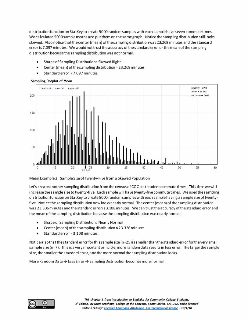
distribution function on StatKey to create 5000 random samples with each sample have seven commute times. We calculated 5000 sample means and put them on the same graph. Notice the sampling distribution still looks skewed. Also notice that the center (mean) of the sampling distribution was 23.268 minutes and the standard error is 7.097 minutes. We would not trust the accuracy of the standard error or the mean of the sampling distribution because the sampling distribution was not normal.
• Shape of Sampling Distribution: Skewed Right • Center (mean) of the sampling distribution ≈ 23.268 minutes • Standard error ≈ 7.097 minutes.
Mean Example 2: Sample Size of Twenty-Five from a Skewed Population
Let’s create another sampling distribution from the census of COC stat student commute times. This time we will increase the sample size to twenty-five. Each sample will have twenty-five commute times. We used the sampling distribution function on StatKey to create 5000 random samples with each sample having a sample size of twenty-five. Notice the sampling distribution now looks nearly normal. The center (mean) of the sampling distribution was 23.336 minutes and the standard error is 3.108 minutes. We can trust the accuracy of the standard error and the mean of the sampling distribution because the sampling distribution was nearly normal.
• Shape of Sampling Distribution: Nearly Normal • Center (mean) of the sampling distribution ≈ 23.336 minutes • Standard error ≈ 3.108 minutes.
Notice also that the standard error for this sample size (n=25) is smaller than the standard error for the very small sample size (n=7). This is a very important principle, more random data results in less error. The larger the sample size, the smaller the standard error, and the more normal the sampling distribution looks.
More Random Data → Less Error → Sampling Distribution becomes more normal
This chapter is from Introduction to Statistics for Community College Students, 1st Edition, by Matt Teachout, College of the Canyons, Santa Clarita, CA, USA, and is licensed
under a “CC-By” Creative Commons Attribution 4.0 International license – 10/1/18
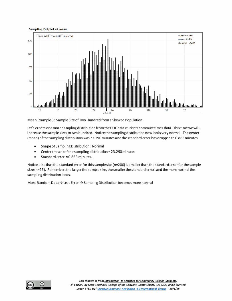
Mean Example 3: Sample Size of Two Hundred from a Skewed Population
Let’s create one more sampling distribution from the COC stat students commute times data. This time we will increase the sample sizes to two hundred. Notice the sampling distribution now looks very normal. The center (mean) of the sampling distribution was 23.290 minutes and the standard error has dropped to 0.863 minutes.
• Shape of Sampling Distribution: Normal • Center (mean) of the sampling distribution ≈ 23.290 minutes • Standard error ≈ 0.863 minutes.
Notice also that the standard error for this sample size (n=200) is smaller than the standard error for the sample size (n=25). Remember, the larger the sample size, the smaller the standard error, and the more normal the sampling distribution looks.
More Random Data → Less Error → Sampling Distribution becomes more normal

This chapter is from Introduction to Statistics for Community College Students, 1st Edition, by Matt Teachout, College of the Canyons, Santa Clarita, CA, USA, and is licensed
under a “CC-By” Creative Commons Attribution 4.0 International license – 10/1/18
Summary: If a population is skewed, it seems we need a larger sample size, for the sampling distribution to look normal. As the sample size increases, the standard error decreases, and the sampling distribution looks more normal. This is the idea behind the “Central Limit Theorem”. A common rule when dealing with means is that if the population is skewed the sample size should be at least 30 for the sampling distribution for sample means to look normal.
Central Limit Theorem: If the sample size is sufficiently large, the sampling distribution for sample means will have a normal shape even if the population is skewed.
Key Question: What would happen if the population was already normal?
Mean Example 4: Sampling Distribution from a normal population.
Let’s now look at an example of a census with a normal shape. In the Fall 2015 semester we took a census of all of the statistics students at COC and asked them their heights in inches. We will assume this was an unbiased census. This population looked very normal with a population mean average height of 66.511 inches and a population standard deviation of 4.787 inches. For this example we will focus on the mean.

This chapter is from Introduction to Statistics for Community College Students, 1st Edition, by Matt Teachout, College of the Canyons, Santa Clarita, CA, USA, and is licensed
under a “CC-By” Creative Commons Attribution 4.0 International license – 10/1/18
Now let’s see what happens if we take thousands of samples from this population. We will start with small sample sizes of 10 stat students at a time.
We took 3000 random samples each of size ten and calculated 3000 sample means to create this sampling distribution. Notice a few key things.
• The sample means are different. We see sampling variability in action. The population mean was 66.511 inches but the sample means could be anywhere from about 62 inches to 72 inches. Sample statistics are different and usually very different than the population parameter
• Even though we have a very small sample size of ten, the sampling distribution still looks normal. This means that the center (mean) of the sampling distribution and the standard error are relatively accurate even for a sample size of ten.

This chapter is from Introduction to Statistics for Community College Students, 1st Edition, by Matt Teachout, College of the Canyons, Santa Clarita, CA, USA, and is licensed
under a “CC-By” Creative Commons Attribution 4.0 International license – 10/1/18
• The center of the sampling distribution (66.516 inches) is very close to the population mean of (66.511 inches)
• We have calculated the standard error of 1.501. For a sample size of 10, typical sample means are within 1.501 inches of the population mean. The margin of error is probably closer to 3 inches (2 x standard error).
Sample Mean Summary
Let’s summarize our findings about sample means from random samples.
1. If the population is skewed, we will need a sample size of at least 30 or higher in order to insure that our sampling distribution for sample means will be nearly normal.
2. If the population is already normal, then the sampling distribution for sample means will be normal for any sample size.
Important note about sample size:
Even though the minimum requirement for sample means is a sample size of 30 or above, this does not mean we are happy with a data set of only 30. Remember less data results in more error. For random data, the bigger the sample size the better. Thirty is just the bare minimum requirement to insure that the sampling distribution for sample means will look nearly normal.
Standard Deviation Example 1: Standard Deviation and Variance
Remember that the sample variance is the square of the standard deviation. Statisticians often opt to estimate variability in sample variances instead of standard deviation. Later, we can take the square root of the variance estimates to get the standard deviation.
If the population was skewed, what is the shape of sampling distributions for sample standard deviations? Are there any sample size requirements for estimating sample standard deviations? What if the population was already normal?
In the last section, we looked at the COC work hours census data from Fall 2015. We see that the population standard deviation is 12.969 hours per week. We created a sampling distribution of 251 random samples and calculate 251 random sample standard deviations. Each sample had a sample size of 50. If we put all of the sample standard deviations on the same graph, we can create a sampling distribution for sample standard deviations.

This chapter is from Introduction to Statistics for Community College Students, 1st Edition, by Matt Teachout, College of the Canyons, Santa Clarita, CA, USA, and is licensed
under a “CC-By” Creative Commons Attribution 4.0 International license – 10/1/18
Notice that while a sample size of 50 would be large enough to ensure a sampling distribution of sample means to be normal, it does not insure a sampling distribution of sample standard deviations to be normal. If the population is skewed, the sampling distribution for sample standard deviations will tend to be skewed.
Sample Standard Deviation and Sample Variance Summary
Let’s summarize our findings about sample standard deviations and sample variance from random samples.
1. A sampling distributions of sample variance is usually skewed right. Later we will see that if the population is normal, the sampling distribution for sample variance will follow a skewed right Chi-Squared distribution. Requirements for traditional techniques for estimating population variance or population standard deviations usually require the population to be normal no matter what the sample size is. If the population was not normal, then we would have to resort to different technique l ike bootstrapping.
Sample Proportion Example 1:
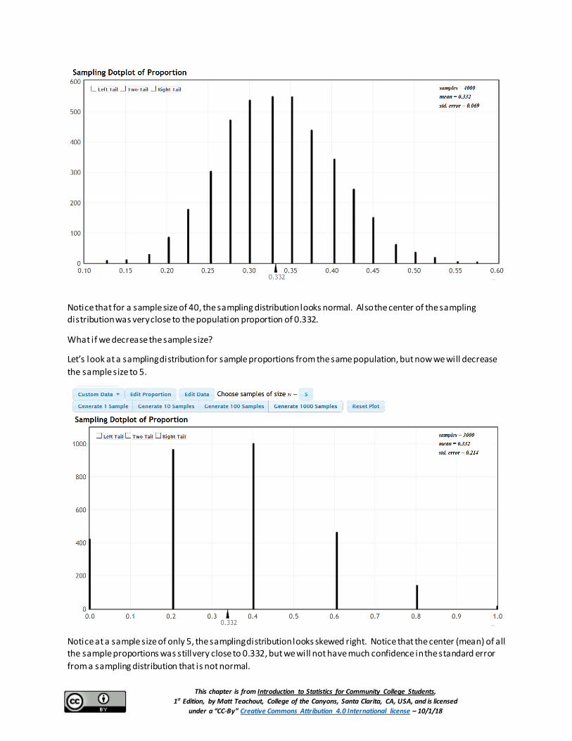
In the last section we looked at the fall 2015 census of COC stat students and found that the population percentage that attend the Canyon Country campus was 0.332 or 33.2%. Here is a sampling distribution of thousands of random samples taken from the COC statistics student census. Remember the population proportion was 0.332.
This chapter is from Introduction to Statistics for Community College Students, 1st Edition, by Matt Teachout, College of the Canyons, Santa Clarita, CA, USA, and is licensed
under a “CC-By” Creative Commons Attribution 4.0 International license – 10/1/18
Notice that for a sample size of 40, the sampling distribution looks normal. Also the center of the sampling distribution was very close to the population proportion of 0.332.
What if we decrease the sample size?
Let’s look at a sampling distribution for sample proportions from the same population, but now we will decrease the sample size to 5.
Notice at a sample size of only 5, the sampling distribution looks skewed right. Notice that the center (mean) of all the sample proportions was still very close to 0.332, but we will not have much confidence in the standard error from a sampling distribution that is not normal.

This chapter is from Introduction to Statistics for Community College Students, 1st Edition, by Matt Teachout, College of the Canyons, Santa Clarita, CA, USA, and is licensed
under a “CC-By” Creative Commons Attribution 4.0 International license – 10/1/18
So what sample size insures a normal sampling distribution for sample proportions?
The “At Least Ten” rule
It turns out that for random categorical data, the random sample should have at least ten successes and at least ten failures. We should have at least 10 statistics students from the Canyon Country campus and at least 10 that are not from the Canyon Country campus to insure that the sampling distribution will look normal.
Notice if we only had a random sample of five stat students, it is impossible to get at least ten from Canyon Country and at least ten not from Canyon Country.
There is no minimum sample size requirement for categorical data because the population proportion will be different in each situation.
Why did the sampling distribution for samples of size 40 work?
If we know the population proportion (𝜋𝜋), here is a common formula for estimating the number of success and failures in random categorical sample data:
Expected number of success for sample size (𝑛𝑛): 𝑛𝑛(𝜋𝜋) Expected number of failures for sample size (𝑛𝑛): 𝑛𝑛(1 −𝜋𝜋)
For a sample size of 40, will we be l ikely to get ten successes and ten failures? If the population proportion for Canyon Country is 0.332, we are l ikely to get about 13 students from Canyon Country and 27 students not from Canyon Country.
𝑛𝑛(𝜋𝜋) = 40(0.332) = 13.28
𝑛𝑛(1 −𝜋𝜋) = 40(1−0.332) = 40(0.668) = 26.72
Important Note: Remember we rarely have an unbiased census, so we may have no idea what the population proportion is. All we have is random sample data. In that case, you will want your random categorical sample data to have at least ten success and at least ten failures. That does not mean twenty!
Summary of Sampling Distributions for sample proportions (sample %)
• Categorical data does not have a shape. Yet if we compute thousands of sample proportions and put them on the same graph, the sampling distribution will have a shape.
• To insure the sampling distribution for sample proportions will be normal we want to have at least ten successes and at least ten failures in our random categorical sample data.

This chapter is from Introduction to Statistics for Community College Students, 1st Edition, by Matt Teachout, College of the Canyons, Santa Clarita, CA, USA, and is licensed
under a “CC-By” Creative Commons Attribution 4.0 International license – 10/1/18
Key Question#1: Why is it so important for a sampling distribution to be normal?
We will discuss this in greater detail in later sections, but here are two of the main reasons.
• Remember standard error is the standard deviation of the sampling distribution and measures the typical distance from the mean (center) of the sampling distribution. Neither the standard error nor the center (mean) of the sampling distribution are very accurate unless the sampling distribution is normal.
• Before computers were invented, statisticians relied on formulas to understand sampling variability, calculate standard error and estimate population parameters. Many of these formulas are based on normal curves and are not accurate if the sampling distribution is not normal. This is why conditions or assumptions for sample means and sample proportions are often tied to making sure the sampling distribution is normal when estimating population parameters.
Key Question#2: Is there a way to estimate a population parameter and understand sampling variability when the sampling distribution is not normal?
• Yes. Computer technology may be used to understand sampling variability in the case when our sampling distribution is not likely to be normal. Techniques like bootstrapping and randomized simulation were invented to be able to understand sampling variability, calculate standard error, and estimate or check population parameters when the sampling distribution is not normal. We will discuss these techniques in later chapters.
Problem Set Section 3C Directions: Answer the following questions about sample size requirements and the shape of sampling distributions.
1. Why is it important for a sampling distribution for sample means or sample proportions to be normal?
2. What conditions should be met to insure that a sampling distribution of sample proportions is normal?
3. State the Central Limit Theorem and explain the ideas behind it.
4. Suppose the population is not normal. If we increase the sample size, what will happen to the standard error and the shape of the sampling distribution of sample means?
5. Suppose the population is not normal. If we decrease the sample size, what will happen to the standard error and the shape of the sampling distribution of sample means?
6. Suppose the population is not normal. What conditions should be met in order to insure that a sampling distribution of sample means is normal?
7. If the population is normal, will the sampling distribution for sample means look normal for very small sample sizes?
8. Median averages, variance and standard deviation can have very irregular looking sampling distributions. This can make traditional formula calculations difficult. Is there a way to study sampling variability and estimate population parameters when a sampling distribution is not normal or when traditional formulas are not accurate?

This chapter is from Introduction to Statistics for Community College Students, 1st Edition, by Matt Teachout, College of the Canyons, Santa Clarita, CA, USA, and is licensed
under a “CC-By” Creative Commons Attribution 4.0 International license – 10/1/18
Section 3D – Introduction to Confidence Intervals Vocabulary
Population: The collection of all people or objects to be studied.
Census: Collecting data from everyone in a population.
Sample: Collecting data from a small subgroup of the population.
Statistic: A number calculated from sample data in order to understand the characteristics of the data. For example, a sample mean average, a sample standard deviation, or a sample percentage.
Parameter: A number that describes the characteristics of a population like a population mean or a population percentage. Can be calculated from an unbiased census, but is often just a guess about the population.
Point Estimate: When someone takes a sample statistic and then claims that it is the population parameter.
Margin of Error: Total distance that a sample statistic might be from the population parameter. For normal sampling distributions and a 95% confidence interval, the margin of error is approximately twice as large as the standard error.
Standard Error: The standard deviation of a sampling distribution. The distance that typical sample statistics are from the center of the sampling distribution. Since the center of the sampling distributions is usually close to the population parameter, the standard error tells us how far typical sample statistics are from the population parameter.
Confidence Interval: Two numbers that we think a population parameter is in between.
95% Confident: 95% of confidence intervals contain the population value and 5% of confidence intervals do not contain the population value.
90% Confident: 90% of confidence intervals contain the population value and 10% of confidence intervals do not contain the population value.
99% Confident: 99% of confidence intervals contain the population value and 1% of confidence intervals do not contain the population value.
What if the population percentage of people worldwide have congestive heart failure (CHF)? What is the population mean average salary of every working adult in Japan? Estimating population parameters is very important if we are to understand the world around us.
Estimating Population Parameters
There are two ways for finding a population parameter, an unbiased census or the center of a sampling distribution from thousands of large random samples. If you collect data from everyone in your population and have not incorporated bias into the data, then you have collected an unbiased census. In that case, you know the entire population. Unbiased census data can be used to find population parameters l ike the population mean (µ), the population standard deviation (𝜎𝜎), or the population proportion (𝜋𝜋). Simply calculate the mean or proportion or standard deviation of the census and you know your population parameter.

This chapter is from Introduction to Statistics for Community College Students, 1st Edition, by Matt Teachout, College of the Canyons, Santa Clarita, CA, USA, and is licensed
under a “CC-By” Creative Commons Attribution 4.0 International license – 10/1/18
We also learned that if you collect many large random samples from a population, you can create a sampling distribution. The center of the sampling distribution is usually a very good estimate of the population parameter.
This is not what happens usually in the real world. Populations may have millions of people, making it virtually impossible to take a census (unless you are the government). Most data scientists simply cannot collect a census from large populations. Random samples are usually very difficult to collect and can be expensive. Therefore, it is rare to see someone collect many random samples from the same population. Certainly not thousands of random samples. So we often cannot create a sampling distribution from the population either.
A person analyzing data usually has one large random sample. So the question is, can we estimate a population parameter with one large random sample?
Remember the principle of sampling variability.
Sampling Variability: Random sample statistics will usually be different from each other and different from the population parameter.
Every time we take a random sample we will get something different. The sample statistic you calculate from random sample data will almost always be off from the population parameter. Remember there will always be a margin of error.
Key: If all you have is one random sample, you will not be able to find the population parameter. The sample statistic you calculate will be off from the real population parameter.
If we have one random sample, can we estimate the population parameter at least? Yes, but we should be careful how we label it.
Point Estimates
Point Estimate: Some people take the random sample statistic and then just tell us in their article or report that the sample statistic is the population parameter.
Most of the time, when someone in an article gives us a population parameter, it usually is not the actual population parameter. It is a point estimate. They took some sample data, calculated the sample mean, and then tell us that the sample mean is the population mean. As you can imagine this creates a lot of confusion. Many people read articles and think the author knows the exact population mean or the exact population percentage, when in fact the number the author is quoting came from a sample. It is important to be aware of this. A good scientific report will usually make this distinction.
Good Point Estimate: “We tested a random sample of people for high cholesterol and found that 31.7% of the sample had high cholesterol. So we estimate that the population percentage of people worldwide with high cholesterol is about 31.7% with a 1.2% margin of error.”
Bad Point Estimate: “The population percentage of people worldwide that have high cholesterol is 31.7%.”
The second example shows what most articles say. It can be very confusing for most people since they believe that the author knows the population percentage for everyone worldwide. They do not realize it was just a sample percentage. We know from our study of sampling distributions and sampling variability that this sample percentage can be very far off from the real population percentage.
This chapter is from Introduction to Statistics for Community College Students, 1st Edition, by Matt Teachout, College of the Canyons, Santa Clarita, CA, USA, and is licensed
under a “CC-By” Creative Commons Attribution 4.0 International license – 10/1/18
Confidence Intervals
A sample statistic will usually be off from the population parameter. In other words, the sample statistic has a margin of error.
Margin of Error: The distance that a sample statistic might be from the population parameter.
It is relatively easy to calculate margin of error if already know the population parameter. Remember we rarely know the population parameter in the real world. It can be very difficult to estimate margin of error when you do not know the population parameter. Many mathematicians and statisticians put a lot of thought into finding formulas that would estimate the margin of error. We will go over some of these famous margin of error formulas throughout the chapter.
If you know the margin of error and the sampling distribution was relatively normal or symmetric, then you can use the margin of error to create a confidence interval.
Confidence Interval: Two numbers that we think a population parameter is in between.
When all you have is one random sample, you will not be able to find the population parameter exactly, but you can find two numbers that we think the population parameter may be in between. This is called a “confidence interval”. For example, we may know what the population percentage is, but we think it is between 10.2% and 13.6%.
Here is a common formula for calculating a confidence interval.
Sample Statistic ± Margin of Error
Example 1: Suppose we look at a random sample of gas mileage (miles per gallon) for various cars. We want to estimate the population mean average mpg for all cars in the world. The sample mean (𝑥𝑥𝑥) was 24.761 mpg but remember this does not mean that the population mean is 24.761. Using a formula, we were able to calculate the margin of error for this sample to be 2.152 mpg. So what would the confidence interval be?
Sample Statistic ± Margin of Error
𝑥𝑥𝑥 ± Margin of Error
24.761 mpg ± 2.152 mpg
Lower Limit: 24.761 – 2.152 = 22.609 mpg
Upper Limit: 24.761 + 2.152 = 26.913 mpg
So a sample mean average gas mileage of 24.761 mpg tells us that the population mean average gas mileage for cars could be in between 22.609 mpg and 26.913 mpg.
Confidence Intervals can be written in three ways: interval notation, inequality notation, or just give the sample statistic and margin of error. In this example here are the three ways the confidence interval may be written.
Interval Notation: ( 22.609 mpg , 26.913 mpg) Most computer programs write their confidence intervals in interval notation. This does not mean (x,y) like in algebra. It means the population parameter could be any of the millions of numbers in between 22.609 mpg and 26.913 mpg.

This chapter is from Introduction to Statistics for Community College Students, 1st Edition, by Matt Teachout, College of the Canyons, Santa Clarita, CA, USA, and is licensed
under a “CC-By” Creative Commons Attribution 4.0 International license – 10/1/18
Inequality Notation: 22.609 mpg < µ < 26.913 mpg Remember this interval was trying to find two numbers that the population mean (µ) is in between. That is exactly what this says.
Sample Statistic and Margin of Error: 24.761 mpg (± 2.152 mpg error) Many scientific journals or articles write it this way. They write the sample statistic as their point estimate with the margin of error.
Example 2: In the article earlier we were looking for the percentage of people worldwide with high cholesterol. What would the confidence interval be for this problem?
“We tested a random sample of people for high cholesterol and found that 31.7% of the sample had high cholesterol. There was a 1.2% margin of error.”
When calculating confidence intervals from a percentage, we usually convert the sample percentage into a sample proportion (𝑝𝑝𝑝). We should also convert the margin of error into a proportion.
31.7% = 0.317
1.2% = 0.012
Sample Statistic ± Margin of Error
𝑝𝑝𝑝 ± Margin of Error
0.317 ± 0.012
Lower Limit: 0.317 – 0.012 = 0.305
Upper Limit: 0.317 + 0.012 = 0.329
We can convert these proportion back into percentages if we wish. Notice that we can write the confidence interval in three ways again. Remember a population proportion can be written with the letter “p” or “π”.
Interval Notation: ( 0.305 , 0.329 ) or ( 30.5% , 32.9% ) Inequality Notation: 0.305 < π < 0.329 or 30.5% < π < 32.9% Sample Statistic and Margin of Error: 31.7% ( ± 1.2% error)
You should be comfortable converting percentages into proportions and proportions into percentages. Notice that when calculating the upper and lower l imits we could have added and subtracted the percentages and got the same answer.
Lower Limit: 31.7% – 1.2% = 30.5%
Upper Limit: 31.7% + 1.2% = 32.9%
So a sample percentage of 31.7% does not tell us that the population percentage. It tells us that the population percentage could be in between 30.5% and 32.9%.
Important Note: Never add or subtract a proportion and a percentage. Yes, they are equivalent, but they are not the same. Either add and subtract the proportions, or add and subtract the percentages.
Never do this!! 11.9 ± 0.017

This chapter is from Introduction to Statistics for Community College Students, 1st Edition, by Matt Teachout, College of the Canyons, Santa Clarita, CA, USA, and is licensed
under a “CC-By” Creative Commons Attribution 4.0 International license – 10/1/18
In the last two examples, how confident are we about these results? Confidence Levels
When calculating confidence intervals, it is important to know what “confidence level” was used. A confidence level is not an abstract feeling about how confident you are. It is tied to the mathematical calculation of the margin of error. The most common confidence levels are 90%, 95% and 99%, with 95% being by far the most common. Whenever you ask a computer to calculate a confidence interval you must choose what level you want to use. Usually it is 95%.
Think of it this way. The more confident you are, the larger the margin of error and the wider you make the confidence interval. That way you are more l ikely to have the actual population parameter in between the two numbers. The less confident you are the smaller the margin of error and the narrower the confidence interval. I l ike to think of the confidence level as a catcher’s mitt in baseball. If I want to be 90% confident that I catch the ball (catch the population parameter), I will use a regular sized catcher’s mitt. If I want to be 95% confident I catch the ball, I will use a jumbo-sized catcher’s mitt. If I want to be 99% confident that I catch the ball, I will use a huge soccer net.
90% confidence level → Small margin of error → Narrow confidence interval (Regular sized Mitt)
95% confidence level → Larger margin of error → Wider confidence interval (Jumbo sized Mitt)
99% confidence level → Extremely Large margin of error → Very wide confidence interval (Soccer Net)
Example: Earlier we looked at creating a confidence interval to estimate two numbers that we think the population mean average gas mileage (mpg) is in between. The following printout shows the calculation for 90%, 95% and 99% confidence levels. Notice that as the confidence level increases, the margin of errors are increasing the numbers in the confidence intervals are getting farther apart.

This chapter is from Introduction to Statistics for Community College Students, 1st Edition, by Matt Teachout, College of the Canyons, Santa Clarita, CA, USA, and is licensed
under a “CC-By” Creative Commons Attribution 4.0 International license – 10/1/18
Confidence Interval Sentence
Computers can calculate confidence intervals. The job of a data analyst, data scientist or statistician is to explain. In other words, the sentences are very important. Whenever we write a sentence to explain a confidence interval, we should always state the confidence level that was used. For one-population confidence intervals we should also give the two numbers that the population parameter is in between.
One Population Confidence Interval Sentence:
“We are (90%, 95% or 99%) confident that the population parameter is in between # and #”.
Here is the sentence for the 90% confidence interval estimate of the population mean average mpg. Remember in quantitative data, you can round the answers to one more decimal point than is present in the original data. (In this case, since the original sample data mpg values were rounded to the tenths place, we can round the confidence intervals to the hundredths place.) If you do not know the accuracy of your data, it is better not to round the numbers.
We are 90% confident that population mean average gas mileage for all cars is between 22.97 mpg and 26.55 mpg.
Here is the sentence for the 95% confidence interval estimate of the population mean average mpg. We rounded the Statcato answers to the hundredths place.
We are 95% confident that population mean average gas mileage for all cars is between 22.61 mpg and 27.64 mpg.
Here is the sentence for the 99% (rounded) confidence interval estimate of the population mean average mpg.
We are 99% confident that population mean average gas mileage for all cars is between 21.88 mpg and 26.91 mpg.

This chapter is from Introduction to Statistics for Community College Students, 1st Edition, by Matt Teachout, College of the Canyons, Santa Clarita, CA, USA, and is licensed
under a “CC-By” Creative Commons Attribution 4.0 International license – 10/1/18
Here is the sentence for the genetic trait population percentage confidence interval. We will assume it was a 95% confidence level.
We are 95% confident that population percentage of all people worldwide that have high cholesterol is between 30.5% and 32.9%.
Understanding Confidence Levels
Here are the definitions of confidence. Notice that these definitions are not talking about a “feeling” about confidence. They are also not talking about being sure that the population parameter is in between the exact two numbers in a confidence interval. So what do these mean?
95% Confident: 95% of confidence intervals contain the population value and 5% of confidence intervals do not contain the population value.
90% Confident: 90% of confidence intervals contain the population value and 10% of confidence intervals do not contain the population value.
99% Confident: 99% of confidence intervals contain the population value and 1% of confidence intervals do not contain the population value.
These definitions are talking about many samples, many confidence intervals. In essence, a sampling distribution.
Example 1: 90% confidence level sampling distribution
Work Hours per Week for working COC Statistics Students (Fall 2015 semester)
In a previous section, we created a sampling distribution of sample means for the work hours of statistics students. We did not use students that said they work “zero” hours. To understand confidence levels, we are going to take it a step further. Instead of just taking many random samples and calculating many sample means, we are going to use StatKey to calculate many confidence intervals. All of the confidence intervals will have a 90% confidence level. We used a sample size of 30 this time.

This chapter is from Introduction to Statistics for Community College Students, 1st Edition, by Matt Teachout, College of the Canyons, Santa Clarita, CA, USA, and is licensed
under a “CC-By” Creative Commons Attribution 4.0 International license – 10/1/18
Let’s see if we understand what we are looking at. The dark l ine indicates the population mean of 27.283 hours of work per week. If the population mean is in between the two numbers in the confidence level, then the confidence interval is green. This indicates that the confidence interval contains the population parameter. If the population mean is not in between the two numbers in the confidence level, then the confidence interval is red. This indicates that the confidence interval does not contain the population parameter.
Notice when we use a 90% confidence level, about 90% of them were green (contained the population parameter) and about 10% of them were red (did not contain the population parameter). In other words not all confidence intervals contain the population parameter! This is what the definition of 90% confidence is talking about. If we take many random samples, and create many confidence intervals, about 90% of the confidence intervals will have the population parameter in between the two numbers and 10% of them will not.
Notice that the green and red l ines describing the confidence interval have a lot of variability. This is sampling variability at work. Random samples will always be different. That means that the confidence interval numbers will also be different for every random sample.

This chapter is from Introduction to Statistics for Community College Students, 1st Edition, by Matt Teachout, College of the Canyons, Santa Clarita, CA, USA, and is licensed
under a “CC-By” Creative Commons Attribution 4.0 International license – 10/1/18
Also notice that the number of green confidence intervals was not exactly 90%. In fact it was 91% for the first hundred samples. 90% is a l imit. This means that because of sampling variability, the exact percentage of green confidence intervals will fluctuate. As the number of samples increase, the number usually gets closer and closer to 90%.
Example 2: 95% confidence level sampling distribution
Work Hours per Week for working COC Statistics Students (Fall 2015 semester)
Now we will set the confidence levels to 95%. We calculated many confidence intervals and all of them have a 95% confidence level. Notice that the percentage of green confidence intervals that contain the population mean average is now approaching 95%. It is actually 96% for these first 100 samples, but as the number of samples increase, the percentage will get closer to 95%. Also notice that the percentage of red confidence intervals that do not contain the population mean average is now approaching 5%. It is actually 4% for these first 100 samples, but as the number of samples increase, the percentage will get closer to 5%. This again is what the definition of 95% confidence is talking about. If we create many 95% confidence intervals, about 95% of them will be green and contain the population parameter, and about 5% of them will be red and not contain the population parameter.
Example 3: 99% confidence level sampling distribution
Work Hours per Week for working COC Statistics Students (Fall 2015 semester)
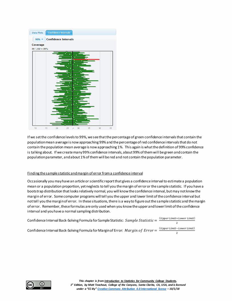
This chapter is from Introduction to Statistics for Community College Students, 1st Edition, by Matt Teachout, College of the Canyons, Santa Clarita, CA, USA, and is licensed
under a “CC-By” Creative Commons Attribution 4.0 International license – 10/1/18
If we set the confidence levels to 99%, we see that the percentage of green confidence intervals that contain the population mean average is now approaching 99% and the percentage of red confidence intervals that do not contain the population mean average is now approaching 1%. This again is what the definition of 99% confidence is talking about. If we create many 99% confidence intervals, about 99% of them will be green and contain the population parameter, and about 1% of them will be red and not contain the population parameter.
Finding the sample statistic and margin of error from a confidence interval
Occasionally you may have an article or scientific report that gives a confidence interval to estimate a population mean or a population proportion, yet neglects to tell you the margin of error or the sample statistic. If you have a bootstrap distribution that looks relatively normal, you will know the confidence interval, but may not know the margin of error. Some computer programs will tell you the upper and lower limit of the confidence interval but not tell you the margin of error. In these situations, there is a way to figure out the sample statistic and the margin of error. Remember, these formulas are only used when you know the upper and lower l imit of the confidence interval and you have a normal sampling distribution.
Confidence Interval Back-Solving Formula for Sample Statistic: 𝑆𝑆𝑆𝑆𝑆𝑆𝑝𝑝𝑆𝑆𝑆𝑆 𝑆𝑆𝑆𝑆𝑆𝑆𝑆𝑆𝑆𝑆𝑠𝑠𝑆𝑆𝑆𝑆𝑆𝑆= (𝑈𝑈𝑈𝑈𝑈𝑈𝑈𝑈𝑈𝑈 𝐿𝐿𝐿𝐿𝐿𝐿𝐿𝐿𝐿𝐿+𝐿𝐿𝐿𝐿𝐿𝐿𝑈𝑈𝑈𝑈 𝐿𝐿𝐿𝐿𝐿𝐿𝐿𝐿𝐿𝐿)
2
Confidence Interval Back-Solving Formula for Margin of Error: 𝑀𝑀𝑆𝑆𝑀𝑀𝑀𝑀𝑆𝑆𝑛𝑛 𝑜𝑜𝑜𝑜 𝐸𝐸𝑀𝑀𝑀𝑀𝑜𝑜𝑀𝑀= (𝑈𝑈𝑈𝑈𝑈𝑈𝑈𝑈𝑈𝑈 𝐿𝐿𝐿𝐿𝐿𝐿𝐿𝐿𝐿𝐿−𝐿𝐿𝐿𝐿𝐿𝐿𝑈𝑈𝑈𝑈 𝐿𝐿𝐿𝐿𝐿𝐿𝐿𝐿𝐿𝐿)
2

This chapter is from Introduction to Statistics for Community College Students, 1st Edition, by Matt Teachout, College of the Canyons, Santa Clarita, CA, USA, and is licensed
under a “CC-By” Creative Commons Attribution 4.0 International license – 10/1/18
Example 1: Bootstrap Confidence Interval for Population Mean Average Body Temperature
Bootstrapping is a technique for calculating confidence intervals. The following bootstrap confidence interval was calculated from a random sample of 50 adult body temperatures in degrees Fahrenheit. The upper and lower l imits for the confidence interval are given at the bottom right and left of the bootstrap distribution. The confidence level is given in the middle of the bootstrap distribution. So the 95% confidence interval is (98.050 ℉, 98.472 ℉).
Confidence Interval Sentence: We are 95% confident that the population mean average body temperature of human adults is between 98.050℉ and 98.472℉.
StatKey did tell us that the sample mean was 98.26℉, but notice that we do not know the margin of error. This is a perfect time to use the back-solving formula for margin of error.
M𝑆𝑆𝑀𝑀𝑀𝑀𝑆𝑆𝑛𝑛 𝑜𝑜𝑜𝑜 𝐸𝐸𝑀𝑀𝑀𝑀𝑜𝑜𝑀𝑀 = (𝑈𝑈𝑈𝑈𝑈𝑈𝑈𝑈𝑈𝑈 𝐿𝐿𝐿𝐿𝐿𝐿𝐿𝐿𝐿𝐿−𝐿𝐿𝐿𝐿𝐿𝐿𝑈𝑈𝑈𝑈 𝐿𝐿𝐿𝐿𝐿𝐿𝐿𝐿𝐿𝐿)
2 =
(98.472−98.050)
2 =
(0.422)
2= 0.211 ℉
Let’s check the sample statistic formula and see how close it is to the actual sample mean.
Sample Statistic (mean) = (𝑈𝑈𝑈𝑈𝑈𝑈𝑈𝑈𝑈𝑈 𝐿𝐿𝐿𝐿𝐿𝐿𝐿𝐿𝐿𝐿+𝐿𝐿𝐿𝐿𝐿𝐿𝑈𝑈𝑈𝑈 𝐿𝐿𝐿𝐿𝐿𝐿𝐿𝐿𝐿𝐿)
2 =
(98.472+98.050)
2 =
(196.522)
2= 98.261 ℉
Notice the sample statistic is very close to the actual sample mean of 98.26 ℉.

This chapter is from Introduction to Statistics for Community College Students, 1st Edition, by Matt Teachout, College of the Canyons, Santa Clarita, CA, USA, and is licensed
under a “CC-By” Creative Commons Attribution 4.0 International license – 10/1/18
Example 2: An article claims that the population percentage of young adults ages 18-25 years in the U.S. that have depression is in between 9.59% and 12.27%. This is a confidence interval. We will assume they used a 95% confidence level. What was the sample proportion and the margin of error? Again, this would be a good time to use the back-solving formulas. Remember to either use the proportions or the percentages but do not add or subtract a proportion and a percentage.
M𝑆𝑆𝑀𝑀𝑀𝑀𝑆𝑆𝑛𝑛 𝑜𝑜𝑜𝑜 𝐸𝐸𝑀𝑀𝑀𝑀𝑜𝑜𝑀𝑀 = (𝑈𝑈𝑈𝑈𝑈𝑈𝑈𝑈𝑈𝑈 𝐿𝐿𝐿𝐿𝐿𝐿𝐿𝐿𝐿𝐿−𝐿𝐿𝐿𝐿𝐿𝐿𝑈𝑈𝑈𝑈 𝐿𝐿𝐿𝐿𝐿𝐿𝐿𝐿𝐿𝐿)
2 =
(0.1227−0.0959)
2 =
(0.0268)
2= 0.0134 (or 1.34%)
M𝑆𝑆𝑀𝑀𝑀𝑀𝑆𝑆𝑛𝑛 𝑜𝑜𝑜𝑜 𝐸𝐸𝑀𝑀𝑀𝑀𝑜𝑜𝑀𝑀 = (𝑈𝑈𝑈𝑈𝑈𝑈𝑈𝑈𝑈𝑈 𝐿𝐿𝐿𝐿𝐿𝐿𝐿𝐿𝐿𝐿−𝐿𝐿𝐿𝐿𝐿𝐿𝑈𝑈𝑈𝑈 𝐿𝐿𝐿𝐿𝐿𝐿𝐿𝐿𝐿𝐿)
2 =
(12.27%−9.59%)
2 =
(2.68%)
2= 1.34% (or 0.0134 as a proportion)
Sample Statistic (proportion) = (𝑈𝑈𝑈𝑈𝑈𝑈𝑈𝑈𝑈𝑈 𝐿𝐿𝐿𝐿𝐿𝐿𝐿𝐿𝐿𝐿+𝐿𝐿𝐿𝐿𝐿𝐿𝑈𝑈𝑈𝑈 𝐿𝐿𝐿𝐿𝐿𝐿𝐿𝐿𝐿𝐿)
2 =
(0.1227+0.0959)
2 =
(0.2186)
2= 0.1093 (or 10.93%)
Sample Statistic (percentage) = (𝑈𝑈𝑈𝑈𝑈𝑈𝑈𝑈𝑈𝑈 𝐿𝐿𝐿𝐿𝐿𝐿𝐿𝐿𝐿𝐿+𝐿𝐿𝐿𝐿𝐿𝐿𝑈𝑈𝑈𝑈 𝐿𝐿𝐿𝐿𝐿𝐿𝐿𝐿𝐿𝐿)
2 =
(12.27%+9.59%)
2 =
(21.86%)
2= 10.93% (or 0.1093)
Summary of Confidence Intervals
• Be aware of point estimates. When a person claims to know the exact population parameter in an article, they probably just calculated a sample statistic and are telling you it is the population parameter. We only know the population parameter if we have collected a census or if we have collected many, many random samples and look for the center of the sampling distribution. We can never know the exact population parameter from a large population if all we have is one random sample. If we have one random sample, all we can do is estimate the population parameter with a confidence interval.
• A confidence interval is two numbers that we think a population parameter is in between.
• Remember, a confidence interval should never be calculated from a census. If you already know the population parameter, there is no need to estimate it with a confidence interval. Confidence interval are calculated when we only have random sample data and need to estimate the population parameter.
• It is important to know what confidence levels were used. 90%, 95% and 99% are all sometimes used, though 95% is the most common. Remember, these levels do not refer to a feeling of confidence about one confidence interval. They are part of the confidence interval calculation and refer to the process of calculating thousands of confidence intervals.
• Here are definitions of 90%, 95%, and 99% confidence. These definitions imply that not all confidence intervals contain the population parameter. Sometimes the population parameter will not be in between the two numbers in the confidence interval. 90% Confident: 90% of confidence intervals contain the population value and 10% of confidence intervals do not contain the population value. 95% Confident: 95% of confidence intervals contain the population value and 5% of confidence intervals do not contain the population value. 90% Confident: 99% of confidence intervals contain the population value and 1% of confidence intervals do not contain the population value.
This chapter is from Introduction to Statistics for Community College Students, 1st Edition, by Matt Teachout, College of the Canyons, Santa Clarita, CA, USA, and is licensed
under a “CC-By” Creative Commons Attribution 4.0 International license – 10/1/18
• The margin of error is how far we think the sample statistic is from the population parameter. A common formula that is sometimes used to calculate a confidence interval is the sample statistic ± margin of error.
• Be able to explain the confidence interval. Here is a common sentence used for one-population confidence intervals: We are (90%, 95% or 99%) confident that the population parameter (mean, proportion, median, standard deviation, or variance) is in between # and #.
• If you know the upper and lower limit of a confidence interval from a normal sampling distribution, you can use these back solving formulas to find the sample statistic and the margin of error.
𝑆𝑆𝑆𝑆𝑆𝑆𝑝𝑝𝑆𝑆𝑆𝑆 𝑆𝑆𝑆𝑆𝑆𝑆𝑆𝑆𝑆𝑆𝑠𝑠𝑆𝑆𝑆𝑆𝑆𝑆 = (𝑈𝑈𝑝𝑝𝑝𝑝𝑆𝑆𝑀𝑀 𝐿𝐿𝑆𝑆𝑆𝑆𝑆𝑆𝑆𝑆+ 𝐿𝐿𝑜𝑜𝐿𝐿𝑆𝑆𝑀𝑀 𝐿𝐿𝑆𝑆𝑆𝑆𝑆𝑆𝑆𝑆)
2
𝑀𝑀𝑆𝑆𝑀𝑀𝑀𝑀𝑆𝑆𝑛𝑛 𝑜𝑜𝑜𝑜 𝐸𝐸𝑀𝑀𝑀𝑀𝑜𝑜𝑀𝑀 = (𝑈𝑈𝑝𝑝𝑝𝑝𝑆𝑆𝑀𝑀 𝐿𝐿𝑆𝑆𝑆𝑆𝑆𝑆𝑆𝑆− 𝐿𝐿𝑜𝑜𝐿𝐿𝑆𝑆𝑀𝑀 𝐿𝐿𝑆𝑆𝑆𝑆𝑆𝑆𝑆𝑆)
2
Problem Set Section 3D (For #1-5) Add and subtract the given sample statistic and margin of error to find the confidence interval estimate of the population value. Then write the confidence interval using both inequality notation and using interval notation. Now write a sentence explaining the confidence interval to someone.
Confidence interval = Sample Statistic ± Margin of Error
1. “What percent of the adult population is infected with this disease?” sample percentage = 4.9% margin of error = 1.3% (Found with 95% confidence level.)
2. “What is the population mean average height for men?” sample mean = 68.335 inches margin of error = 1.293 inches (Found with 99% confidence level.)
3. What is the population standard deviation for the systolic blood pressure in women? (Assume there was a normal sampling distribution.) sample standard deviation = 17.11 mm of Hg margin of error = 3.31 mm of Hg (Found with 90% confidence level.)
4. What percentage of left handed people get migraine headaches? sample proportion = 0.088 margin of error = 0.027 (Found with 95% confidence level.)
5. What is the mean average price of a used mustang car in thousands of dollars? sample mean = 15.98 thousand dollars margin of error = 3.78 thousand dollars (Found with 90% confidence level.)
(For #6-10) Write a sentence explaining each of the following confidence intervals. Then use the following formulas to identify the sample statistic ( p̂ or x̅ or s ) and the margin of error.
Sample Statistic = (𝑢𝑢𝑈𝑈𝑈𝑈𝑈𝑈𝑈𝑈 𝑙𝑙𝐿𝐿𝐿𝐿𝐿𝐿𝐿𝐿+𝑙𝑙𝐿𝐿𝐿𝐿𝑈𝑈𝑈𝑈 𝑙𝑙𝐿𝐿𝐿𝐿𝐿𝐿𝐿𝐿)2
Margin of Error = (𝑢𝑢𝑈𝑈𝑈𝑈𝑈𝑈𝑈𝑈 𝑙𝑙𝐿𝐿𝐿𝐿𝐿𝐿𝐿𝐿−𝑙𝑙𝐿𝐿𝐿𝐿𝑈𝑈𝑈𝑈 𝑙𝑙𝐿𝐿𝐿𝐿𝐿𝐿𝐿𝐿)2

This chapter is from Introduction to Statistics for Community College Students, 1st Edition, by Matt Teachout, College of the Canyons, Santa Clarita, CA, USA, and is licensed
under a “CC-By” Creative Commons Attribution 4.0 International license – 10/1/18
6. A 95% confidence interval estimate of the population proportion of fat in the milk from Jersey cows is (0.046 , 0.052).
7. A 99% confidence interval estimate of the population mean number of miles is 13.4 miles < µ < 17.2 miles.
8. A 90% confidence interval estimate of the population proportion of people who will vote for the Independent party candidate is 0.068 < p < 0.083
9. A 95% confidence interval estimate of the population mean amount of milk in gallons is ( 48.7 , 58.4 )
10. A 99% confidence interval estimate of the population standard deviation for the height of men in inches is 2.34 < σ < 2.87 (assume there was a normal sampling distribution)
(#11-16) Go to www.matt-teachout.org and click on “statistics” and then “data sets”. Open the “coffee data” and copy and Columbian Mild price data. Now go to www.lock5stat.com and click on the “StatKey” button. Under the “sampling distribution” menu click on “mean”. Under edit data, paste the Columbian Mild coffee data. Click on “samples of size n” and put in 30. Turn off the button that says “first column is identifier” as we have only a single column of data. Now click ok. You are now ready to create your sampling distribution. This time we want the computer to create a confidence interval for each sample it takes. On the right side of the screen, click on the button that says confidence intervals and set the confidence level to 95%. StatKey will take a random sample from the population data, find the sample mean and place a dot for the sample mean in the distribution. It will also create a confidence interval from that sample mean. Remember that the population mean price for the Columbian mild coffee was 134.338 cents per pound. StatKey will keep track of whether the true population mean is actually contained in the confidence interval or not. Green means the confidence interval did contain the population value and red means that the confidence interval did not contain the population value. Now answer the following questions.
11. Notice the confidence intervals for sample means were different for each random sample. Discuss the implications of sampling variability on the accuracy of a confidence interval from a random sample.
12. Did all the confidence intervals contain the population mean 134.338 cents per pound? What does it mean that the interval “contained” or “captured” the population mean?
13. How many total random samples did you take? How many of them contained the population mean 134.338 cents? What percent of the confidence intervals contained the population mean?
14. How many confidence intervals did not contain the population mean 134.338 cents? What percent of the confidence intervals did not contain the population mean?
15. As the number of random samples increased, did the percentage of confidence intervals that contained the population mean get closer or farther away from 95%? Why do you think that is?
16. Here is the definition of 95% confidence: “95% of confidence intervals contain the population parameter and 5% do not contain the population parameter”. Explain this definition of 95% confidence in your own words.
(#17-22) Assume a fair coin has a 50% (0.5) chance of getting tails. If we take samples from that population, the sample proportions will usually not be 0.5. We want to look at lots of proportion confidence intervals from sample proportions. Go to www.lock5stat.com and click on the “StatKey” button. Under the “sampling distribution” menu click on “proportion”. Under “edit proportion”, put in 0.5 and then click ok. You are now ready to create your sampling distribution. We want the computer to create a confidence interval for each sample proportion. On the
This chapter is from Introduction to Statistics for Community College Students, 1st Edition, by Matt Teachout, College of the Canyons, Santa Clarita, CA, USA, and is licensed
under a “CC-By” Creative Commons Attribution 4.0 International license – 10/1/18
right side of the screen, click on the button that says confidence intervals and set the confidence level to 90%. StatKey will take a random sample from the population data, find the sample proportion and place a dot for the sample proportion in the distribution. It will also create a confidence interval from that sample sample. Remember that the population proportion for a fair coin is 0.5 (50%). StatKey will keep track of whether the true population proportion is actually contained in the confidence interval or not. Green means the confidence interval did contain the population value and red means that the confidence interval did not contain the population value. Now answer the following questions.
17. Notice the confidence intervals for sample proportions were different for each random sample. Discuss the implications of sampling variability on the accuracy of a confidence interval created from a random sample proportion.
18. Did all the confidence intervals contain the population proportion of 0.5? What does it mean that the interval “contained” or “captured” the population parameter?
19. How many total confidence intervals did you make? How many of them contained the population proportion 0.5? What percent of the confidence intervals contained the population proportion 0.5?
20. How many of the confidence intervals did not contain the population proportion 0.5? What percent of the confidence intervals did not contain the population proportion 0.5?
21. As the number of random samples increased, did the percentage of confidence intervals that contained the population proportion get closer or farther away from 90%? Why do you think that is?
22. Here is the definition of 90% confidence: “90% of confidence intervals contain the population parameter and 10% do not contain the population parameter”. Explain this definition of 90% confidence in your own words.
Section 3E – One Population Confidence Intervals Vocabulary
Population: The collection of all people or objects to be studied.
Census: Collecting data from everyone in a population.
Sample: Collecting data from a small subgroup of the population.
Statistic: A number calculated from sample data in order to understand the characteristics of the data. For example, a sample mean average, a sample standard deviation, or a sample percentage.
Parameter: A number that describes the characteristics of a population like a population mean or a population percentage. Can be calculated from an unbiased census, but is often just a guess about the population.
Sampling Distribution: Take many random samples from a population, calculate a sample statistic like a mean or percent from each sample and graph all of the sample statistics on the same graph. The center of the sampling distribution is a good estimate of the population parameter.
Sampling Variability: Random samples values and sample statistics are usually different than each other and usually different than the population parameter.

This chapter is from Introduction to Statistics for Community College Students, 1st Edition, by Matt Teachout, College of the Canyons, Santa Clarita, CA, USA, and is licensed
under a “CC-By” Creative Commons Attribution 4.0 International license – 10/1/18
Point Estimate: When someone takes a sample statistic and then claims that it is the population parameter.
Margin of Error: Total distance that a sample statistic might be from the population parameter. For normal sampling distributions and a 95% confidence interval, the margin of error is approximately twice as large as the standard error.
Standard Error: The standard deviation of a sampling distribution. The distance that typical sample statistics are from the center of the sampling distribution. Since the center of the sampling distributions is usually close to the population parameter, the standard error tells us how far typical sample statistics are from the population parameter.
Confidence Interval: Two numbers that we think a population parameter is in between. Can be calculated by either a bootstrap distribution or by adding and subtracting the sample statistic and the margin of error.
95% Confident: 95% of confidence intervals contain the population value and 5% of confidence intervals do not contain the population value.
90% Confident: 90% of confidence intervals contain the population value and 10% of confidence intervals do not contain the population value.
99% Confident: 99% of confidence intervals contain the population value and 1% of confidence intervals do not contain the population value.
Bootstrapping: Taking many random samples values from one original real random sample with replacement.
Bootstrap Sample: A simulated sample created by taking many random samples values from one original real random sample with replacement.
Bootstrap Statistic: A statistic calculated from a bootstrap sample.
Bootstrap Distribution: Putting many bootstrap statistics on the same graph in order to simulate the sampling variability in a population, calculate standard error, and create a confidence interval. The center of the bootstrap distribution is the original real sample statistic.
In the last section, we saw that if we have only one random sample from a population, we will not be able to find the population parameter exactly. The best we can do is calculate a confidence interval, that is two numbers that we think the population parameter is in between.
In this section, we will look at some of the famous formulas that statisticians use to estimate population parameters with confidence intervals. We will also look at sample data conditions in order to ensure the accuracy of the formula.
If our sampling distribution is normal, most one-population confidence interval formulas start from the following.
Sample Statistic ± Margin of Error
Early mathematicians and statisticians thought a lot about how to estimate the margin of error when you do not know the population parameter. The key was the sampling distribution. If a sampling distribution looked normal, then the empirical rule would suggest that the middle 95% would correspond to two standard deviations above and below the center. This gave rise to another common formula.
Sample Statistic ± (2 × Standard Error)

This chapter is from Introduction to Statistics for Community College Students, 1st Edition, by Matt Teachout, College of the Canyons, Santa Clarita, CA, USA, and is licensed
under a “CC-By” Creative Commons Attribution 4.0 International license – 10/1/18
Critical Value Z-scores
What is the “2” representing in the following formula. It seems it is counting how many standard errors one is from the mean (center) of the sampling distribution. Does this remind you of a statistic we previously learned?
If you recall, the Z-score measures the number of standard deviations from the mean. So the “2” is really a Z-score. This gave rise to the idea of replacing the “2” with a Z-score. The Z-score can be adapted for 90%, 95% or 99%. Remember 2 standard deviation is just an approximation for 95%. If that is the case, can we get a more accurate number for 95%?
Using a normal calculator, we can calculate the Z-score for 90%, 95% and 99% confidence. These are very famous and are often referred to as “critical value Z-scores” or "𝑍𝑍𝑐𝑐" for short.
Go to www.lock5stat.com and open StatKey. Under the “theoretical distributions” menu, click on “normal”. If the mean is 0 and the standard deviation is 1, then this will calculate Z-scores. Click the “two-tail” button. The first Z-score calculated is for 95%.
This is the most famous of all the critical value Z-scores. Remember, for the middle 95%, the empirical rule indicates that it will be “about” two standard deviations. It turns out, 1.96 standard deviations is more accurate. Notice that just l ike the confidence intervals have an upper limit and lower l imit, so does the Z-score critical values. For 95% confidence, we can replace the ±2 in the formula with ±1.96.
What about 90% confidence intervals? Go back to the normal calculator in StatKey and click on the “0.95” in the middle. Change it to 0.9 (90%).

This chapter is from Introduction to Statistics for Community College Students, 1st Edition, by Matt Teachout, College of the Canyons, Santa Clarita, CA, USA, and is licensed
under a “CC-By” Creative Commons Attribution 4.0 International license – 10/1/18
Notice the Z-score for 90% confidence intervals is ±1.645. Notice that as the confidence interval decreases from 95% to 90%, the Z-score gets lower. This will cause the margin of error to decrease and the confidence interval to get narrower.
What about 99% confidence intervals? Go back to the normal calculator in StatKey and change the middle proportion into 0.99 (99%).
Notice the Z-score for 99% confidence intervals is ±2.576. So instead of being 1.645 standard errors away or 1.96 standard errors away, now we are 2.576 standard errors away. As the confidence interval increases from 95% to 99%, the Z-score gets larger. This will cause the margin of error to increase and the confidence interval to get wider.
Here are the famous critical value Z-scores.

This chapter is from Introduction to Statistics for Community College Students, 1st Edition, by Matt Teachout, College of the Canyons, Santa Clarita, CA, USA, and is licensed
under a “CC-By” Creative Commons Attribution 4.0 International license – 10/1/18
• 90% confidence level: Z = ± 1.645 • 95% confidence level: Z = ± 1.96 • 99% confidence level: Z = ± 2.576
Let’s summarize the progress of our one-population confidence interval formula. It is important to remember that these formulas only work if our sampling distribution looks normal. Z-scores calculate the number of standard deviations (standard errors) from the mean in a perfectly normal curve.
Sample Statistic ± Margin of Error
Sample Statistic ± (2 × Standard Error)
Sample Statistic ± (Z × Standard Error)
Statisticians discovered that as long as the sampling distribution was normal, the Z-scores were pretty accurate for proportion (percentage) confidence intervals. The famous critical value Z-scores are still used to this day to calculate a confidence interval estimate of a population proportion (percentage).
One-Population Proportion Confidence Interval
Before computers were invented, it was very difficult to make sampling distributions. Yet it was vital to understanding sample statistics and calculating standard error. Early mathematicians and statisticians invented formulas to estimate the standard error.
Standard Error Estimation Formula for Proportions = �𝑈𝑈�(1−𝑈𝑈�)𝑛𝑛
Sample Proportion = p̂ Sample Size = n
So now we can finish our estimation formula for a confidence interval estimate of the population proportion. In order to estimate the margin of error, we multiply the standard error by the number of standard errors (Z-score).
Sample Statistic ± Margin of Error Sample Statistic ± (2 × Standard Error) Sample Statistic ± (Z × Standard Error)
p̂ ± �𝑍𝑍�𝑈𝑈�(1−𝑈𝑈�)𝑛𝑛
�
Example 1: Calculating the confidence interval for a proportion
A random sample of 54 bears in a region of California showed that 19 of them were female. Find the sample proportion and use the formula above to calculate a 95% confidence interval estimate for the population proportion of female bears in this region of California.

This chapter is from Introduction to Statistics for Community College Students, 1st Edition, by Matt Teachout, College of the Canyons, Santa Clarita, CA, USA, and is licensed
under a “CC-By” Creative Commons Attribution 4.0 International license – 10/1/18
Sample Proportion (𝑝𝑝𝑝) = 𝐴𝐴𝐿𝐿𝐿𝐿𝑢𝑢𝑛𝑛𝐿𝐿 𝐿𝐿𝑜𝑜 𝐹𝐹𝑈𝑈𝐿𝐿𝐹𝐹𝑙𝑙𝑈𝑈 𝐵𝐵𝑈𝑈𝐹𝐹𝑈𝑈𝐵𝐵𝑆𝑆𝐹𝐹𝐿𝐿𝑈𝑈𝑙𝑙𝑈𝑈 𝑆𝑆𝐿𝐿𝑆𝑆𝑈𝑈
= 1954
≈ 0.352
Critical Value Z-score for 90% Confidence = ± 1.96
Now we will replace the Z-score with 1.96 and p̂ with 0.352 and n with 54 into our formula and work it out. Remember to follow order of operations. Notice the standard error estimate is 0.065 (6.5%) and the margin of error estimate is 0.127 (12.7%).
p̂ ± �𝑍𝑍�𝑈𝑈�(1−𝑈𝑈�)𝑛𝑛
�
0.352 ± �1.96�0.352(1−0.352)54
�
0.352 ± �1.96�0.352(0.648)54
�
0.352 ± (1.96 × 0.065)
0.352 ± (0.127)
0.352 – 0.127 < Population Proportion of Female Bears (𝜋𝜋) < 0.352 + 0.127
0.225 < Population Proportion of Female Bears (𝜋𝜋) < 0.479
We are 95% confident that between 22.5% and 47.9% of all bears in this region of California are female.
Note: While it is important to understand formulas, data scientist today rely on computers to calculate confidence intervals. It is very difficult to calculate confidence intervals from large data sets with a formula and a calculator. The job of a data scientist, statistician, or data analyst is understand and explain the data, not to spend hours calculating something a computer can do in a split second.
To calculate this confidence interval with Statcato, we will click on the “statistics” menu and then “confidence intervals”. Click on one-population proportion and under summary data, enter 19 for the number of events and 54 for the number of trials. Set the confidence level to 0.95 and click OK.
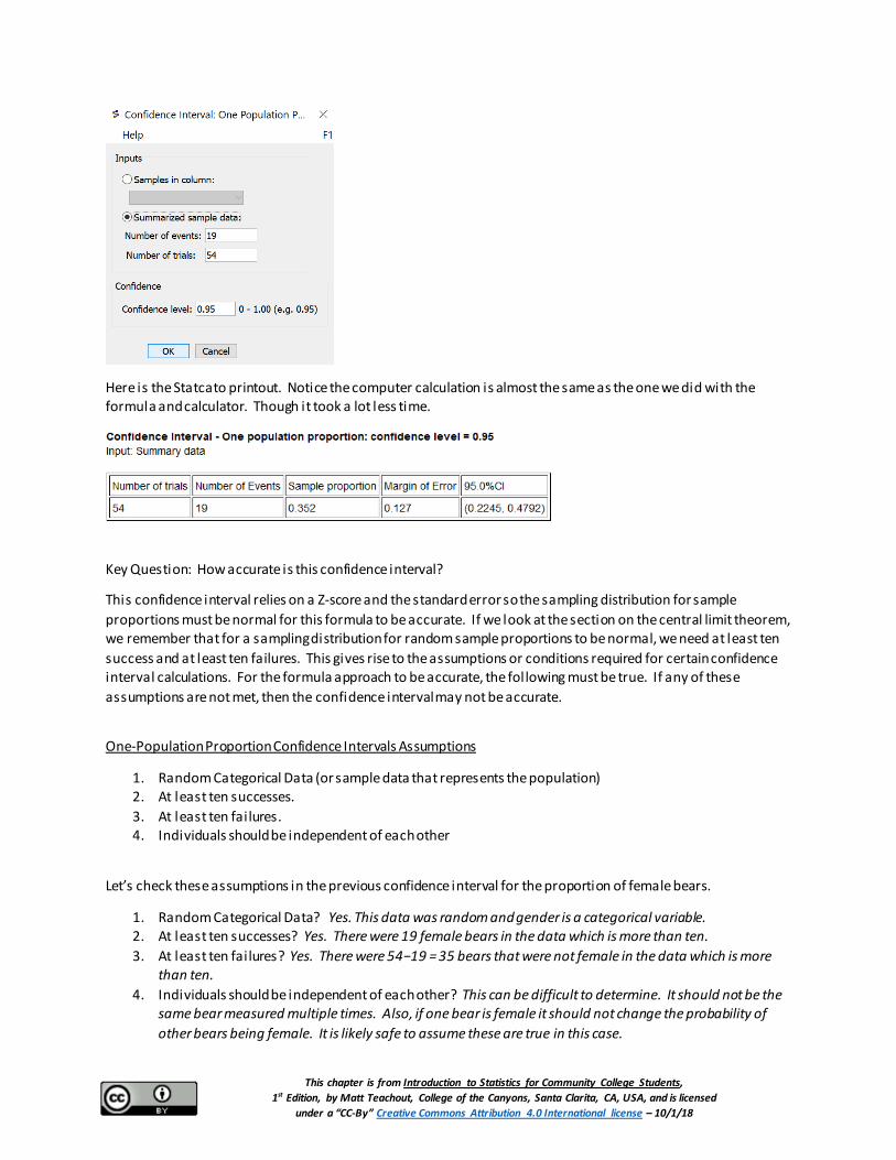
This chapter is from Introduction to Statistics for Community College Students, 1st Edition, by Matt Teachout, College of the Canyons, Santa Clarita, CA, USA, and is licensed
under a “CC-By” Creative Commons Attribution 4.0 International license – 10/1/18
Here is the Statcato printout. Notice the computer calculation is almost the same as the one we did with the formula and calculator. Though it took a lot less time.
Key Question: How accurate is this confidence interval?
This confidence interval relies on a Z-score and the standard error so the sampling distribution for sample proportions must be normal for this formula to be accurate. If we look at the section on the central limit theorem, we remember that for a sampling distribution for random sample proportions to be normal, we need at least ten success and at least ten failures. This gives rise to the assumptions or conditions required for certain confidence interval calculations. For the formula approach to be accurate, the following must be true. If any of these assumptions are not met, then the confidence interval may not be accurate.
One-Population Proportion Confidence Intervals Assumptions
1. Random Categorical Data (or sample data that represents the population) 2. At least ten successes. 3. At least ten failures. 4. Individuals should be independent of each other
Let’s check these assumptions in the previous confidence interval for the proportion of female bears.
1. Random Categorical Data? Yes. This data was random and gender is a categorical variable. 2. At least ten successes? Yes. There were 19 female bears in the data which is more than ten. 3. At least ten failures? Yes. There were 54−19 = 35 bears that were not female in the data which is more
than ten. 4. Individuals should be independent of each other? This can be difficult to determine. It should not be the
same bear measured multiple times. Also, if one bear is female it should not change the probability of other bears being female. It is likely safe to assume these are true in this case.

This chapter is from Introduction to Statistics for Community College Students, 1st Edition, by Matt Teachout, College of the Canyons, Santa Clarita, CA, USA, and is licensed
under a “CC-By” Creative Commons Attribution 4.0 International license – 10/1/18
Overall, it appears the data does satisfy the requirements for using the formula and so the confidence interval will be relatively accurate.
Bootstrapping
Is there a way to make a confidence interval if the data did not meet the assumptions?
It depends on which assumptions. One technique that is sometimes used is called “Bootstrapping”. Bootstrapping does require the sample to be representative of the population. That usually means it was collected randomly. It is also good to have the individuals be independent of each other. As long as you have those two assumptions, you can bootstrap.
Assumptions for Bootstrap Confidence Intervals
• Representative unbiased random sample data. • Individuals should be independent of each other.
Bootstrapping does not use formula for standard error and critical values like Z-scores or T-scores. It calculates the middle 95%, 99% or 90% directly using a bootstrap sampling distribution. Since bootstrapping is not tied to formulas and critical values it does not require the sampling distribution to be normal or to match up with a specific theoretical curve.
The idea of bootstrapping is to create a theoretical population by assuming that the population is just many copies of your one real representative random sample. In practice, bootstrapping uses computers to take thousands for random samples with replacement from your one representative random sample. It randomly selects a value from your data, but puts the value back before picking another value randomly. This allows us to get the same value in a bootstrap sample multiple times. It then calculates the statistic l ike the mean or proportion from all of the bootstrap samples. These are sometimes called “bootstrap statistics”. Putting all the bootstrap statistics on the same graph gives a “bootstrap sampling distribution”. If you find the computer find the cutoffs for the middle 95% of the bootstrap distribution, you have an estimated 95% confidence interval.
Bootstrapping: Taking many random samples values from one original real random sample with replacement.
Bootstrap Sample: A simulated sample created by taking many random samples values from one original real random sample with replacement.
Bootstrap Statistic: A statistic calculated from a bootstrap sample.
Bootstrap Distribution: Putting many bootstrap statistics on the same graph in order to simulate the sampling variability in a population, calculate standard error, and create a confidence interval. The center of the bootstrap distribution is the original real sample statistic.
Female Bears Example
In the last example, we used the traditional Z critical value and standard error formula to create a confidence interval and estimate the population percentage of bears that are female. We could also use a bootstrap. Go to the “Bootstrap Confidence Interval” menu in StatKey at www.lock5stat.com and click on “CI for Single Proportion”. Under “Edit Data” put in the random sample data count (19 female bears) and the total sample size (54 bears). Click “Generate 1000 Samples” a few times. Now click “Two-Tail”. The default is 95%, but you can always change the middle proportion to 99% (0.99) or 90% (0.90) if needed. This problem was a 95% confidence interval, so we will leave the middle proportion as 0.95.

This chapter is from Introduction to Statistics for Community College Students, 1st Edition, by Matt Teachout, College of the Canyons, Santa Clarita, CA, USA, and is licensed
under a “CC-By” Creative Commons Attribution 4.0 International license – 10/1/18
In a bootstrap confidence interval, the upper and lower l imit of the confidence interval are found at the bottom right and left (0.222 and 0.481). Using these numbers, we are 95% confident that the population percentage of bears in this region of California that are female is between 22.2% and 48.1%. Notice that the upper l imit, lower l imit and standard error are very close to what we got by formula or Statcato. Notice that the shape of the bootstrap distribution is very normal. Though the bootstrap does not give us the margin of error l ike Statcato, we can use the formula we learned in the previous section. Remember the standard error and margin of error in this calculation are only reasonably accurate if the distribution is normal. Notice the margin of error is close to what we got by formula or Statcato.
Margin of Error = (𝑈𝑈𝑈𝑈𝑈𝑈𝑈𝑈𝑈𝑈 𝐿𝐿𝐿𝐿𝐿𝐿𝐿𝐿𝐿𝐿−𝐿𝐿𝐿𝐿𝐿𝐿𝑈𝑈𝑈𝑈 𝐿𝐿𝐿𝐿𝐿𝐿𝐿𝐿𝐿𝐿)
2 =
(0.481−0.222)
2 ≈ 0.1295
Key Notes about Bootstrapping
• A bootstrap distribution attempts to estimate and visualize the sampling variability in the population by creating a simulated population. Remember that standard error and margin of error are only accurate if the distribution is normal. So while we can estimate standard error and margin of error from a bootstrap, they may not be accurate if the bootstrap distribution is not normal.
• While a bootstrap distribution may be similar to a true sampling distribution from the population, there are important differences. The center of a bootstrap distribution is the sample statistic from the original real random data set. This makes the bootstrap ideal for estimating the confidence interval. A true sampling distribution is taking thousands of real samples from the population, so the center of a sampling distribution is the population parameter. We should not treat a true sampling distribution from the population the same as a bootstrap. If you have a sampling distribution, then the center can get a very accurate estimate of the population parameter. If you know the population parameter, you do not need a confidence interval. The middle 95% of a sampling distribution from an actual population is not a confidence interval.

This chapter is from Introduction to Statistics for Community College Students, 1st Edition, by Matt Teachout, College of the Canyons, Santa Clarita, CA, USA, and is licensed
under a “CC-By” Creative Commons Attribution 4.0 International license – 10/1/18
Critical Value T-scores
In 1908, a statistician named William Gosset discovered that while Z-scores were very accurate for proportions, they were not very accurate when estimating mean averages, especially if the sample size was small. Small samples should have a larger margin of error than those indicated by Z-scores. To deal with this problem, he invented T-scores. His idea was that each sample size should have a different number of standard deviations. When Gosset invented the T-distribution, he worked for Guinness Beer and was not allowed to publish his work. He therefore published under the pseudonym “student”. To this day, the T-distribution is often called the “Student T-Distribution” since it was invented by a then unknown author named “student”.
T-scores are the same as Z-scores in the sense that they count the number of standard deviations or standard errors from the mean. However, they have a built in error correction for smaller data sets. For very large sample sizes, T-scores and Z-scores are about the same. For example, if we are using a 95% confidence level and our sample size is very large, then the T-score will be close to the Z-score of ± 1.96 standard deviations. When sample sizes are small, the T-scores become significantly greater than the Z-scores. This causes the margin of error to increase for small sample sizes. Remember, less random data should result in more error. We usually use Z-scores when estimating population proportions or percentages. We prefer to use T-scores when estimating population mean averages.
Note: You can use Z-scores for the mean if the sample size is large or if you know the population standard deviation exactly. However, we rarely know the population standard deviation with any certainty, especially when we do not even know the population mean. Also in large sample sizes, the T-scores are still accurate, so you might as well use the T-scores.
Degrees of Freedom
If you recall from previous sections, statistics like variance and standard deviation are based on a sum of squares divided by the degrees of freedom. For one sample, the degrees of freedom is usually equal to one less than the sample size (𝑑𝑑𝑜𝑜 = 𝑛𝑛− 1). Because of this, Gosset organized his T-scores not by sample size, but by degrees of freedom. Gosset calculated his T-scores with calculus and wrote them on charts. Before computers were invented, a statistician would first calculate the degrees of freedom and then look up the correct T-score on these charts. In modern times, T-scores can be easily calculated with computer programs like StatKey.
Example 1: Calculate the T-score critical value for a sample size n = 13 and a 99% confidence level.
Go to www.lock5stat.com and click on “statkey”. Under the “theoretical distributions” menu, click on “t”. Since the sample size is 13, the degrees of freedom will be df = 13−1 = 12. If we click on “two tail” and set the middle proportion to 0.99, we will get the following.

This chapter is from Introduction to Statistics for Community College Students, 1st Edition, by Matt Teachout, College of the Canyons, Santa Clarita, CA, USA, and is licensed
under a “CC-By” Creative Commons Attribution 4.0 International license – 10/1/18
We see from the graph that critical value T-score for 99% confidence and 12 degrees of freedom is ± 3.054. Notice this is larger than the 99% confidence critical value Z-score (± 2.576). For smaller sample sizes the T-scores are significantly greater than the Z-scores.
Example 2: Calculate the T-score critical value for a sample size n = 500 and a 90% confidence level.
Go to www.lock5stat.com and click on “statkey”. Under the “theoretical distributions” menu, click on “t”. Since the sample size is 13, the degrees of freedom will be df = 500−1 = 499. If we click on “two tail” and set the middle proportion to 0.9, we will get the following.
We see from the graph that critical value T-score for 90% confidence and 499 degrees of freedom is ± 1.648. Notice this is very close to the 90% confidence critical value Z-score (± 1.645). For larger sample sizes the T-scores and the Z-scores are about the same.

This chapter is from Introduction to Statistics for Community College Students, 1st Edition, by Matt Teachout, College of the Canyons, Santa Clarita, CA, USA, and is licensed
under a “CC-By” Creative Commons Attribution 4.0 International license – 10/1/18
Summary of Critical Value T-scores
• T-scores (l ike Z-scores) count the number of standard deviations from the mean. In a sampling distribution of sample means, it counts how many standard errors we should be from the center of the sampling distribution for a given confidence level.
• T-scores are different for every sample size. They are usually organized by degrees of freedom. For one-population, the degrees of freedom is usually 𝑑𝑑𝑜𝑜 = 𝑛𝑛− 1.
• T-scores are significantly larger than Z-scores for small sample sizes. The smaller the sample size, the larger the discrepancy between the T-score and Z-score.
• T-scores are about the same as Z-scores for large sample sizes.
One-Population Mean Confidence Interval
Let’s look at the formula for calculating a one-population mean average confidence interval. Many computer programs to this day, still use this formula.
Statisticians estimated the standard error for a sampling distribution for sample means with the following formula. The formula is surprisingly accurate and close to the standard error in an actual sampling distribution.
Standard Error Estimation Formula for Means = 𝐵𝐵√𝑛𝑛
Sample Standard Deviation = s Sample Size = n
Here is the formula for a confidence interval estimate of the population mean. In order to estimate the margin of error, we multiply the standard error by the number of standard errors (T-score).
Sample Statistic ± Margin of Error Sample Mean ± (T × Standard Error)
x̅ ± �𝑇𝑇 𝐵𝐵
√𝑛𝑛�
Example 1: Calculating the confidence interval estimate of a population mean
A random sample of 54 bears in a region of California was taken. The weights of the bears showed a skewed right shape with a sample mean of 182.889 pounds and sample standard deviation of 121.801 pounds. Find the degrees of freedom and the critical value T-score. Then use the formula above to calculate a 99% confidence interval estimate for the population mean average weight of bears in this region of California.
Degrees of Freedom: df = n – 1 = 54 – 1 = 53.
Using the T-score calculator in StatKey we found that the critical Value T-score for 99% Confidence and 53 degrees of freedom is T = ± 2.671

This chapter is from Introduction to Statistics for Community College Students, 1st Edition, by Matt Teachout, College of the Canyons, Santa Clarita, CA, USA, and is licensed
under a “CC-By” Creative Commons Attribution 4.0 International license – 10/1/18
Now we will replace the T-score with 2.671, x̅ with 182.889, n with 54, and s with 121.801 into our formula and work it out. Remember to follow order of operations. Notice the standard error estimate is 16.575 pounds and the margin of error estimate is 44.272 pounds.
x̅ ± �𝑇𝑇 𝐵𝐵
√𝑛𝑛�
182.889 ± 2.671 × 121.801√54
182.889 ± (2.671 × 16.575)
182.889 ± (44.272)
182.889 – 44.272 < Population Mean Average Weight of Bears in Pounds (µ) < 182.889 + 44.272
138.617 pounds < Population Mean Average Weight of Bears in Pounds (µ) < 272.161 pounds
We are 95% confident that the population mean average weight of bears in this region of California is in between 138.617 pounds and 272.161 pounds.
Note: While it is important to understand this formula, it is much easier to calculate this with a computer.
To calculate this confidence interval with Statcato, we will click on the “statistics” menu and then “confidence intervals”. Click on one-population mean and under summary data, enter 182.889 for the mean, 121.801 for the standard deviation, and 54 for the number of trials. Set the confidence level to 0.99 and click OK. If we have the raw data, we could also put in the column “C1” where it says “samples in column”.
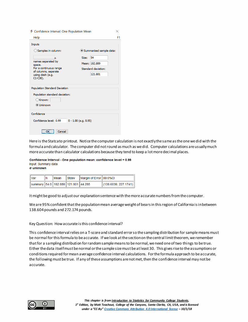
This chapter is from Introduction to Statistics for Community College Students, 1st Edition, by Matt Teachout, College of the Canyons, Santa Clarita, CA, USA, and is licensed
under a “CC-By” Creative Commons Attribution 4.0 International license – 10/1/18
Here is the Statcato printout. Notice the computer calculation is not exactly the same as the one we did with the formula and calculator. The computer did not round as much as we did. Computer calculations are usually much more accurate than calculator calculations because they tend to keep a lot more decimal places.
It might be good to adjust our explanation sentence with the more accurate numbers from the computer.
We are 95% confident that the population mean average weight of bears in this region of California is in between 138.604 pounds and 272.174 pounds.
Key Question: How accurate is this confidence interval?
This confidence interval relies on a T-score and standard error so the sampling distribution for sample means must be normal for this formula to be accurate. If we look at the section on the central l imit theorem, we remember that for a sampling distribution for random sample means to be normal, we need one of two things to be true. Either the data itself must be normal or the sample size must be at least 30. This gives rise to the assumptions or conditions required for mean average confidence interval calculations. For the formula approach to be accurate, the following must be true. If any of these assumptions are not met, then the confidence interval may not be accurate.

This chapter is from Introduction to Statistics for Community College Students, 1st Edition, by Matt Teachout, College of the Canyons, Santa Clarita, CA, USA, and is licensed
under a “CC-By” Creative Commons Attribution 4.0 International license – 10/1/18
One-Population Mean Confidence Intervals Assumptions
1. Random Quantitative Sample Data (or sample data that represents the population) 2. The sample data must be nearly normal or the sample size must be at least 30 3. Individuals should be independent of each other
Let’s check these assumptions in the previous confidence interval for the mean average weight of bears.
1. Random Quantitative Data? Yes. This data was random and weight in pounds is a quantitative variable. 2. The sample data must be nearly normal or the sample size must be at least 30? We see from the
histogram that this data was skewed right, but the sample size was 54 (at least 30). So it does pass the 30 or normal requirement. Remember only one of the two need to be true for it to pass.
3. Individuals should be independent of each other? This can be difficult to determine. It should not be the same bear measured multiple times. These bears were probably tagged so they probably did not accidentally measure the same bear multiple times. Also, one bears weight should not change the probability of other bear having a certain weight. This data may not pass this assumption. Let’s assume we see a bear that is eating well and is very heavy. Then there may be a higher probability of other bears being heavy in the same area.
The data did satisfy the random requirement and the at least 30 or normal requirement. If the data does satisfy the independence assumption, then the data would satisfy the overall requirements for using the formula and so the confidence interval will be relatively accurate.
Could we have calculated this confidence interval with a bootstrap distribution?
Remember, the accuracy of a bootstrap is tied to the quality of the original sample data set. This data set was collected randomly but may fail the independence requirement.
Bear Weight Example
In this last example, we used the traditional T critical value and standard error formula to create a confidence interval and estimate the population mean average weight of bears. We could also use a bootstrap. First go to the “Bear Data” at www.matt-teachout.org and copy the bear weight column of data. Now go to the “Bootstrap Confidence Interval” menu in StatKey at www.lock5stat.com and click on “CI for Single Mean, Median, St.Dev.” Under “Edit Data” paste in the raw quantitative bear weight data. Make sure to check the “Header Row” box since this data set had a title and push “OK”. Click “Generate 1000 Samples” a few times. Now click “Two-Tail”. The default is 95%, but you can change the middle proportion to 99%. This problem was a 99% confidence interval, so we will change the middle proportion to 99% (0.99).
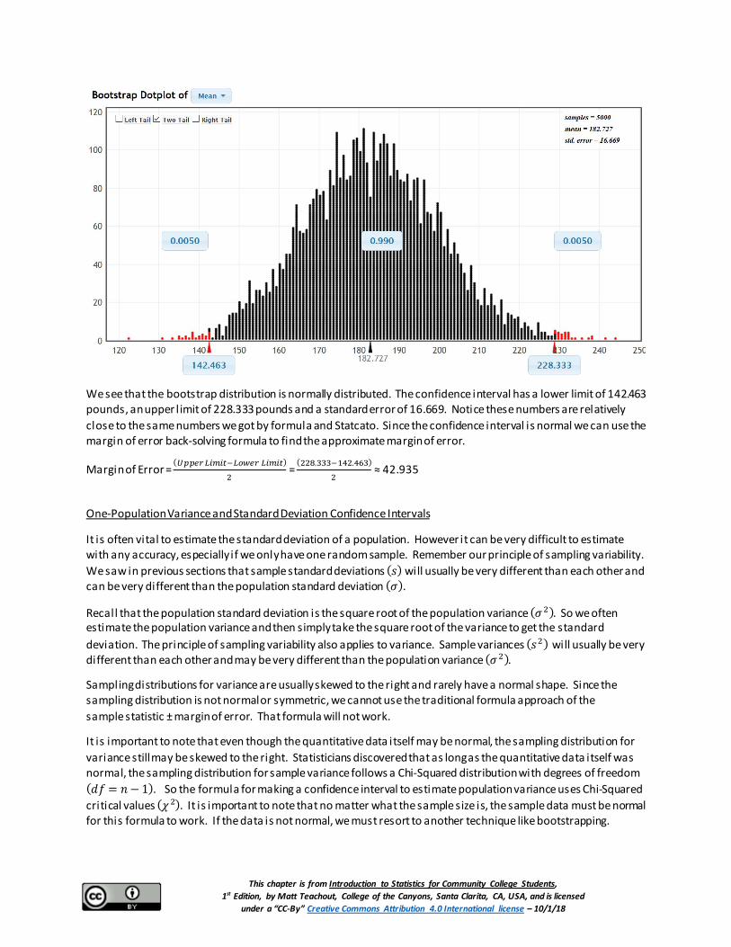
This chapter is from Introduction to Statistics for Community College Students, 1st Edition, by Matt Teachout, College of the Canyons, Santa Clarita, CA, USA, and is licensed
under a “CC-By” Creative Commons Attribution 4.0 International license – 10/1/18
We see that the bootstrap distribution is normally distributed. The confidence interval has a lower limit of 142.463 pounds, an upper l imit of 228.333 pounds and a standard error of 16.669. Notice these numbers are relatively close to the same numbers we got by formula and Statcato. Since the confidence interval is normal we can use the margin of error back-solving formula to find the approximate margin of error.
Margin of Error = (𝑈𝑈𝑈𝑈𝑈𝑈𝑈𝑈𝑈𝑈 𝐿𝐿𝐿𝐿𝐿𝐿𝐿𝐿𝐿𝐿−𝐿𝐿𝐿𝐿𝐿𝐿𝑈𝑈𝑈𝑈 𝐿𝐿𝐿𝐿𝐿𝐿𝐿𝐿𝐿𝐿)
2 =
(228.333−142.463)
2 ≈ 42.935
One-Population Variance and Standard Deviation Confidence Intervals
It is often vital to estimate the standard deviation of a population. However it can be very difficult to estimate with any accuracy, especially if we only have one random sample. Remember our principle of sampling variability. We saw in previous sections that sample standard deviations (𝑠𝑠) will usually be very different than each other and can be very different than the population standard deviation (𝜎𝜎).
Recall that the population standard deviation is the square root of the population variance (𝜎𝜎2). So we often estimate the population variance and then simply take the square root of the variance to get the standard deviation. The principle of sampling variability also applies to variance. Sample variances (𝑠𝑠2) will usually be very different than each other and may be very different than the population variance (𝜎𝜎2).
Sampling distributions for variance are usually skewed to the right and rarely have a normal shape. Since the sampling distribution is not normal or symmetric, we cannot use the traditional formula approach of the sample statistic ± margin of error. That formula will not work.
It is important to note that even though the quantitative data itself may be normal, the sampling distribution for variance still may be skewed to the right. Statisticians discovered that as long as the quantitative data itself was normal, the sampling distribution for sample variance follows a Chi-Squared distribution with degrees of freedom (𝑑𝑑𝑜𝑜 = 𝑛𝑛− 1). So the formula for making a confidence interval to estimate population variance uses Chi-Squared critical values (𝜒𝜒2). It is important to note that no matter what the sample size is, the sample data must be normal for this formula to work. If the data is not normal, we must resort to another technique like bootstrapping.
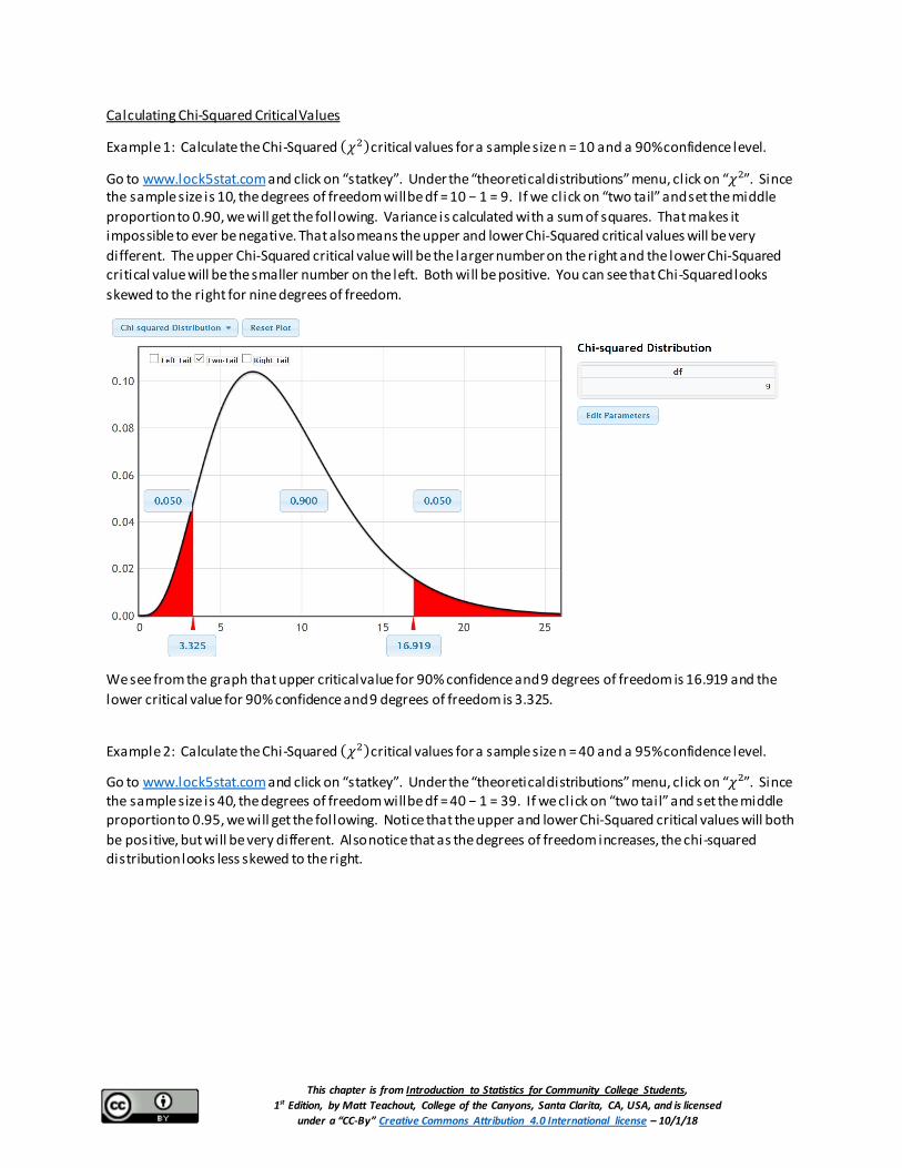
This chapter is from Introduction to Statistics for Community College Students, 1st Edition, by Matt Teachout, College of the Canyons, Santa Clarita, CA, USA, and is licensed
under a “CC-By” Creative Commons Attribution 4.0 International license – 10/1/18
Calculating Chi-Squared Critical Values
Example 1: Calculate the Chi-Squared (𝜒𝜒2) critical values for a sample size n = 10 and a 90% confidence level.
Go to www.lock5stat.com and click on “statkey”. Under the “theoretical distributions” menu, click on “𝜒𝜒2”. Since the sample size is 10, the degrees of freedom will be df = 10 − 1 = 9. If we click on “two tail” and set the middle proportion to 0.90, we will get the following. Variance is calculated with a sum of squares. That makes it impossible to ever be negative. That also means the upper and lower Chi-Squared critical values will be very different. The upper Chi-Squared critical value will be the larger number on the right and the lower Chi-Squared critical value will be the smaller number on the left. Both will be positive. You can see that Chi-Squared looks skewed to the right for nine degrees of freedom.
We see from the graph that upper critical value for 90% confidence and 9 degrees of freedom is 16.919 and the lower critical value for 90% confidence and 9 degrees of freedom is 3.325.
Example 2: Calculate the Chi-Squared (𝜒𝜒2) critical values for a sample size n = 40 and a 95% confidence level.
Go to www.lock5stat.com and click on “statkey”. Under the “theoretical distributions” menu, click on “𝜒𝜒2”. Since the sample size is 40, the degrees of freedom will be df = 40 − 1 = 39. If we click on “two tail” and set the middle proportion to 0.95, we will get the following. Notice that the upper and lower Chi-Squared critical values will both be positive, but will be very different. Also notice that as the degrees of freedom increases, the chi-squared distribution looks less skewed to the right.

This chapter is from Introduction to Statistics for Community College Students, 1st Edition, by Matt Teachout, College of the Canyons, Santa Clarita, CA, USA, and is licensed
under a “CC-By” Creative Commons Attribution 4.0 International license – 10/1/18
We see from the graph that upper critical value for 95% confidence and 39 degrees of freedom is 58.121 and the lower critical value for 95% confidence and 39 degrees of freedom is 23.654.
Confidence Interval Formulas for Variance and Standard Deviation
Here is the confidence interval formulas for estimating population variance. Taking the square root gives us the formula for estimating population standard deviation as well. Notice that the upper critical value is on the left and and lower critical value is on the right. When you divide by a larger number, the overall fraction is smaller.
𝐵𝐵2(𝑛𝑛−1)
𝜒𝜒 𝑢𝑢𝑢𝑢𝑢𝑢𝑢𝑢𝑢𝑢2 < Population Variance (𝜎𝜎2) < 𝐵𝐵2(𝑛𝑛−1)
𝜒𝜒 𝑙𝑙𝑙𝑙𝑙𝑙𝑢𝑢𝑢𝑢2
�𝐵𝐵2(𝑛𝑛−1)
𝜒𝜒 𝑢𝑢𝑢𝑢𝑢𝑢𝑢𝑢𝑢𝑢2 < Population Standard Deviation (𝜎𝜎) < �𝐵𝐵2(𝑛𝑛−1)
𝜒𝜒 𝑙𝑙𝑙𝑙𝑙𝑙𝑢𝑢𝑢𝑢2
Example 1: We measured the heights in inches of 40 randomly selected men. The data showed a normal shape. The sample standard deviation was 3.020 inches. Use the Chi-squared critical values and the formulas above to create a 95% confidence interval for the population variance and the population standard deviation.
We calculated the Chi-squared critical values in the previous example. The upper critical value was 58.121 and the lower critical value was 23.654.
Sample Variance (𝑠𝑠2) = (3.020)2 = 9.1204
Degrees of Freedom (𝑛𝑛− 1) = 40 – 1 = 39
𝐵𝐵2(𝑛𝑛−1)
𝜒𝜒 𝑢𝑢𝑢𝑢𝑢𝑢𝑢𝑢𝑢𝑢2 < Population Variance (𝜎𝜎2) < 𝐵𝐵2(𝑛𝑛−1)
𝜒𝜒 𝑙𝑙𝑙𝑙𝑙𝑙𝑢𝑢𝑢𝑢2
9.1204 (40−1)
58.121 < Population Variance (𝜎𝜎2) < 9.1204 (40−1)
23.654
9.1204 (39)
58 .121 < Population Variance (𝜎𝜎2) < 9.1204 (39)
23.654
6.11992 < Population Variance (𝜎𝜎2) < 15.03744

This chapter is from Introduction to Statistics for Community College Students, 1st Edition, by Matt Teachout, College of the Canyons, Santa Clarita, CA, USA, and is licensed
under a “CC-By” Creative Commons Attribution 4.0 International license – 10/1/18
Variance Confidence Interval Sentence: We are 95% confident that the population variance for all men is between 6.11992 and 15.03744 square inches. (Notice that variance is in square units since it is the standard deviation squared.)
If we take the square root of our answers we can get an estimate of the population standard deviation.
√6.11992 < Population Standard Deviation (𝜎𝜎) < √15.03744
2.47 inches < Population Standard Deviation (𝜎𝜎) < 3.88 inches
Standard Deviation Confidence Interval Sentence: We are 95% confident that the population standard deviation for all men is between 2.47 inches and 3.88 inches.
As with all calculations, it is much easier and more accurate to calculate these with a computer program.
In Statcato, we can go to the “Statistics” menu and click on confidence intervals. If we click on “1-population variance” and enter the sample size (40) and sample standard deviation 3.020 under summary data, we get the following. Notice you can also calculate the confidence interval from raw data or by entering the sample variance.
Notice Statcato gave us almost the same confidence intervals for variance and standard deviation as we calculated with the formula.
Here are the assumptions for making a confidence interval to estimate population variance or standard deviation.

This chapter is from Introduction to Statistics for Community College Students, 1st Edition, by Matt Teachout, College of the Canyons, Santa Clarita, CA, USA, and is licensed
under a “CC-By” Creative Commons Attribution 4.0 International license – 10/1/18
One-Population Variance or Standard Deviation Confidence Intervals Assumptions
1. Random Quantitative Sample Data (or sample data that represents the population) 2. The sample data must be normal 3. Individuals should be independent of each other
Does the men’s height example above, meet these assumptions? Let’s check them.
1. Random Quantitative Sample Data (or sample data that represents the population)? Yes. Height is quantitative and this was a random sample.
2. The sample data must be normal? We did not see the histogram, but the problem did state that the data was normal.
3. Individuals should be independent of each other? Yes. A random sample out of a large population will be unlikely to accidently get men that are family members. One man’s height should not change the probability of another man’s height.
Men’s Height Bootstrap Example
Let’s use a bootstrap distribution to estimate the confidence interval for population standard deviation for men’s height. First go to the “Health Data” at www.matt-teachout.org and copy the men’s height column of data. Now go to the “Bootstrap Confidence Interval” menu in StatKey at www.lock5stat.com and click on “CI for Single Mean, Median, St.Dev.” Under “Edit Data” paste in the raw quantitative men’s height data. Make sure to check the “Header Row” box since this data set had a title and push “OK”. Under “Generate Dotplot of” menu click on “St.Dev.” (standard deviation). Now click “Generate 1000 Samples” a few times. Now click “Two-Tail”. Make sure the middle proportion is 0.95 (95%).
Notice that the upper and lower limits of the confidence interval are close to what we got with formula or Statcato.

This chapter is from Introduction to Statistics for Community College Students, 1st Edition, by Matt Teachout, College of the Canyons, Santa Clarita, CA, USA, and is licensed
under a “CC-By” Creative Commons Attribution 4.0 International license – 10/1/18
Problem Set Section 3E Directions: Answer the following questions.
1. What are the assumptions necessary for making a one-population proportion confidence interval?
2. What are the assumptions necessary for making a one-population mean confidence interval?
3. What are the assumptions necessary for making a one-population variance or standard deviation confidence interval?
4. An experiment was conducted to see what percentage of rats would show empathy toward fellow rats in distress. Of the 30 total rats in the study 23 showed empathy. What was the sample proportion? What are the critical value Z-scores for 99% confidence? If you cannot remember them, open StatKey at www.lock5stat.com and go to “theoretical distributions” and then click on “normal”. You can look up the critical value Z-scores. Use the critical values and the given standard error to calculate the margin of error and construct a 99% confidence interval estimate of the population proportion of rats that show empathy. Convert the upper and lower l imits of your confidence interval into percentages.
Sample Proportion = 𝑁𝑁𝑢𝑢𝐿𝐿𝑁𝑁𝑈𝑈𝑈𝑈 𝐿𝐿𝑜𝑜 𝑆𝑆𝑢𝑢𝑐𝑐𝑐𝑐𝑈𝑈𝐵𝐵𝐵𝐵 (𝑈𝑈𝑒𝑒𝑈𝑈𝑛𝑛𝐿𝐿𝐵𝐵)𝑇𝑇𝐿𝐿𝐿𝐿𝐹𝐹𝑙𝑙 𝑆𝑆𝐹𝐹𝐿𝐿𝑈𝑈𝑙𝑙𝑈𝑈 𝑆𝑆𝐿𝐿𝑆𝑆𝑈𝑈
Standard Error ≈ 0.07725
Proportion Confidence Interval Formula: 𝑝𝑝𝑝 ± (𝑀𝑀𝑆𝑆𝑀𝑀𝑀𝑀𝑆𝑆𝑛𝑛 𝑜𝑜𝑜𝑜 𝐸𝐸𝑀𝑀𝑀𝑀𝑜𝑜𝑀𝑀) = 𝑝𝑝𝑝 ± (𝑍𝑍 ×𝑆𝑆𝑆𝑆𝑆𝑆𝑛𝑛𝑑𝑑𝑆𝑆𝑀𝑀𝑑𝑑 𝐸𝐸𝑀𝑀𝑀𝑀𝑜𝑜𝑀𝑀)
a) Sample Proportion =
b) Critical value Z-scores = ±
c) Margin of Error = 𝑍𝑍× 𝑆𝑆𝑆𝑆𝑆𝑆𝑛𝑛𝑑𝑑𝑆𝑆𝑀𝑀𝑑𝑑 𝐸𝐸𝑀𝑀𝑀𝑀𝑜𝑜𝑀𝑀 =
d) Confidence Interval Lower Limit =
e) Confidence Interval Upper Limit =
5. Use the following Statcato printout to check your margin of error and confidence interval answers from the rat empathy data in number 4. Now check the assumptions and write sentences to explain the margin of error and confidence interval.
a) Check each of the assumptions for this problem. Assume the rats were randomly selected. Explain your answers.
One-Population Proportion Confidence Intervals Assumptions

This chapter is from Introduction to Statistics for Community College Students, 1st Edition, by Matt Teachout, College of the Canyons, Santa Clarita, CA, USA, and is licensed
under a “CC-By” Creative Commons Attribution 4.0 International license – 10/1/18
• Random Categorical Sample Data (or sample data that represents the population) • At least ten successes. • At least ten failures. • Individuals should be independent of each other
b) Write a sentence to explain the margin of error in context.
c) Write a sentence to explain the confidence interval in context.
6. A study was done on the effectiveness of l ie detector tests to catch someone that l ies. In a random sample of 48 total l ies, the machine identified only 31 of them. What was the sample proportion? What are the critical value Z-scores for 95% confidence? If you cannot remember them, open StatKey at www.lock5stat.com and go to “theoretical distributions” and then click on “normal”. You can look up the critical value Z-scores. Use the critical values and the given standard error to calculate the margin of error and construct a 95% confidence interval estimate of the population proportion of l ies caught be l ie detector tests. Convert the upper and lower limits of your confidence interval into percentages.
Sample Proportion = 𝑁𝑁𝑢𝑢𝐿𝐿𝑁𝑁𝑈𝑈𝑈𝑈 𝐿𝐿𝑜𝑜 𝑆𝑆𝑢𝑢𝑐𝑐𝑐𝑐𝑈𝑈𝐵𝐵𝐵𝐵 (𝑈𝑈𝑒𝑒𝑈𝑈𝑛𝑛𝐿𝐿𝐵𝐵)𝑇𝑇𝐿𝐿𝐿𝐿𝐹𝐹𝑙𝑙 𝑆𝑆𝐹𝐹𝐿𝐿𝑈𝑈𝑙𝑙𝑈𝑈 𝑆𝑆𝐿𝐿𝑆𝑆𝑈𝑈
Standard Error ≈ 0.0689
Proportion Confidence Interval Formula: 𝑝𝑝𝑝 ± (𝑀𝑀𝑆𝑆𝑀𝑀𝑀𝑀𝑆𝑆𝑛𝑛 𝑜𝑜𝑜𝑜 𝐸𝐸𝑀𝑀𝑀𝑀𝑜𝑜𝑀𝑀) = 𝑝𝑝𝑝 ± (𝑍𝑍 ×𝑆𝑆𝑆𝑆𝑆𝑆𝑛𝑛𝑑𝑑𝑆𝑆𝑀𝑀𝑑𝑑 𝐸𝐸𝑀𝑀𝑀𝑀𝑜𝑜𝑀𝑀)
a) Sample Proportion =
b) Critical value Z-scores = ±
c) Margin of Error = 𝑍𝑍× 𝑆𝑆𝑆𝑆𝑆𝑆𝑛𝑛𝑑𝑑𝑆𝑆𝑀𝑀𝑑𝑑 𝐸𝐸𝑀𝑀𝑀𝑀𝑜𝑜𝑀𝑀 =
d) Confidence Interval Lower Limit =
e) Confidence Interval Upper Limit =
7. Use the following Statcato printout to check your margin of error and confidence interval answers from the l ie detector data in number 6. Now check the assumptions and write sentences to explain the margin of error and confidence interval.
a) Check each of the assumptions for this problem. Explain your answers.
One-Population Proportion Confidence Intervals Assumptions
• Random Categorical Sample Data (or sample data that represents the population) • At least ten successes.

This chapter is from Introduction to Statistics for Community College Students, 1st Edition, by Matt Teachout, College of the Canyons, Santa Clarita, CA, USA, and is licensed
under a “CC-By” Creative Commons Attribution 4.0 International license – 10/1/18
• At least ten failures. • Individuals should be independent of each other
b) Write a sentence to explain the margin of error in context.
c) Write a sentence to explain the confidence interval in context.
8. A random sample of 45 high school students has a normal distribution. The sample mean average ACT exam score was 20.8 with a sample standard deviation of 9.868. What is the degrees of freedom? Open StatKey at www.lock5stat.com and go to “theoretical distributions” and then click on “T”. Look up the critical value T-scores. Use the critical values and the given standard error to calculate the margin of error and construct a 90% confidence interval estimate of the population mean average ACT exam.
Standard Error = 2.47 ACT points
Mean Confidence Interval Formula: 𝑥𝑥𝑥 ± (𝑀𝑀𝑆𝑆𝑀𝑀𝑀𝑀𝑆𝑆𝑛𝑛 𝑜𝑜𝑜𝑜 𝐸𝐸𝑀𝑀𝑀𝑀𝑜𝑜𝑀𝑀) = 𝑥𝑥𝑥 ± (𝑇𝑇× 𝑆𝑆𝑆𝑆𝑆𝑆𝑛𝑛𝑑𝑑𝑆𝑆𝑀𝑀𝑑𝑑 𝐸𝐸𝑀𝑀𝑀𝑀𝑜𝑜𝑀𝑀)
a) Degrees of Freedom = 𝑛𝑛− 1 =
b) Critical value T-scores = ±
c) Margin of Error = 𝑇𝑇× 𝑆𝑆𝑆𝑆𝑆𝑆𝑛𝑛𝑑𝑑𝑆𝑆𝑀𝑀𝑑𝑑 𝐸𝐸𝑀𝑀𝑀𝑀𝑜𝑜𝑀𝑀 =
d) Confidence Interval Lower Limit =
e) Confidence Interval Upper Limit =
9. Use the following Statcato printout to check your margin of error and confidence interval answers from the ACT data in number 8. Now check the assumptions and write sentences to explain the margin of error and confidence interval.
a) Check each of the assumptions for this problem. Explain your answers.
One-Population Mean Confidence Intervals Assumptions
• Random Categorical Sample Data (or sample data that represents the population) • Sample size at least 30 or nearly normal. • Individuals should be independent of each other
b) Write a sentence to explain the margin of error in context.
c) Write a sentence to explain the confidence interval in context.

This chapter is from Introduction to Statistics for Community College Students, 1st Edition, by Matt Teachout, College of the Canyons, Santa Clarita, CA, USA, and is licensed
under a “CC-By” Creative Commons Attribution 4.0 International license – 10/1/18
10. A random sample of body temperatures in degrees Fahrenheit was taken from 50 randomly selected adults. The sample mean temperature of 98.26 ℉and a standard deviation of 0.765 ℉. What is the degrees of freedom? Open StatKey at www.lock5stat.com and go to “theoretical distributions” and then click on “T”. Look up the critical value T-scores. Use the critical values and the given standard error to calculate the margin of error and construct a 95% confidence interval estimate of the population mean average ACT exam.
Standard Error = 0.1082 ℉
Mean Confidence Interval Formula: 𝑥𝑥𝑥 ± (𝑀𝑀𝑆𝑆𝑀𝑀𝑀𝑀𝑆𝑆𝑛𝑛 𝑜𝑜𝑜𝑜 𝐸𝐸𝑀𝑀𝑀𝑀𝑜𝑜𝑀𝑀) = 𝑥𝑥𝑥 ± (𝑇𝑇× 𝑆𝑆𝑆𝑆𝑆𝑆𝑛𝑛𝑑𝑑𝑆𝑆𝑀𝑀𝑑𝑑 𝐸𝐸𝑀𝑀𝑀𝑀𝑜𝑜𝑀𝑀)
a) Degrees of Freedom = 𝑛𝑛− 1 =
b) Critical value T-scores = ±
c) Margin of Error = 𝑇𝑇× 𝑆𝑆𝑆𝑆𝑆𝑆𝑛𝑛𝑑𝑑𝑆𝑆𝑀𝑀𝑑𝑑 𝐸𝐸𝑀𝑀𝑀𝑀𝑜𝑜𝑀𝑀 =
d) Confidence Interval Lower Limit =
e) Confidence Interval Upper Limit =
11. Use the following Statcato printout to check your margin of error and confidence interval answers from the temperature data in number 10. Now check the assumptions and write sentences to explain the margin of error and confidence interval.
a) Check each of the assumptions for this problem. Explain your answers.
One-Population Mean Confidence Intervals Assumptions
• Random Categorical Sample Data (or sample data that represents the population) • Sample size at least 30 or nearly normal. • Individuals should be independent of each other
b) Write a sentence to explain the margin of error in context.
c) Write a sentence to explain the confidence interval in context.

This chapter is from Introduction to Statistics for Community College Students, 1st Edition, by Matt Teachout, College of the Canyons, Santa Clarita, CA, USA, and is licensed
under a “CC-By” Creative Commons Attribution 4.0 International license – 10/1/18
12. A random sample of 45 high school students ACT exams has a normal distribution with a sample standard deviation (𝑠𝑠) of 9.868. What is the sample variance (𝑠𝑠2)? What is the degrees of freedom? Open StatKey at www.lock5stat.com and go to “theoretical distributions” and then click on “𝜒𝜒2”. Look up the Chi-squared critical values. Use the critical values, degrees of freedom (n−1) and sample variance to construct a 90% confidence interval estimate of the population variance for all ACT exams. Take the square root of your variance confidence interval to calculate a 90% confidence interval estimate for the population standard deviation.
Variance Confidence Interval Formula:
𝐵𝐵2(𝑛𝑛−1)
𝜒𝜒 𝑢𝑢𝑢𝑢𝑢𝑢𝑢𝑢𝑢𝑢2 < Population Variance (𝜎𝜎2) < 𝐵𝐵2(𝑛𝑛−1)
𝜒𝜒 𝑙𝑙𝑙𝑙𝑙𝑙𝑢𝑢𝑢𝑢2
a) Sample Variance = (𝑆𝑆𝑆𝑆𝑆𝑆𝑝𝑝𝑆𝑆𝑆𝑆 𝑆𝑆𝑆𝑆𝑆𝑆𝑛𝑛𝑑𝑑𝑆𝑆𝑀𝑀𝑑𝑑 𝐷𝐷𝑆𝑆𝐷𝐷𝑆𝑆𝑆𝑆𝑆𝑆𝑆𝑆𝑜𝑜𝑛𝑛)2 =
b) Degrees of Freedom = 𝑛𝑛− 1 =
c) Chi-squared upper critical value =
d) Chi-squared lower critical value =
e) Variance Confidence Interval =
f) Standard Deviation Confidence Interval =
13. Use the following Statcato printout to check your variance confidence interval answer and your standard deviation confidence interval answer from the random sample ACT data in number 12. Check the assumptions for a variance confidence interval. Remember the data is normally distributed. Write down a sentence to explain the population variance confidence interval. Write down a sentence to explain the population standard deviation confidence intervals.
a) Now check each of the assumptions for this problem. Explain your answers.
One-Population Variance or Standard Deviation Confidence Intervals Assumptions
• Random Quantitative Sample Data (or sample data that represents the population) • The sample data must be normal • Individuals should be independent of each other
b) Write down a sentence to explain the population variance confidence interval.
c) Write down a sentence to explain the population standard deviation confidence interval.
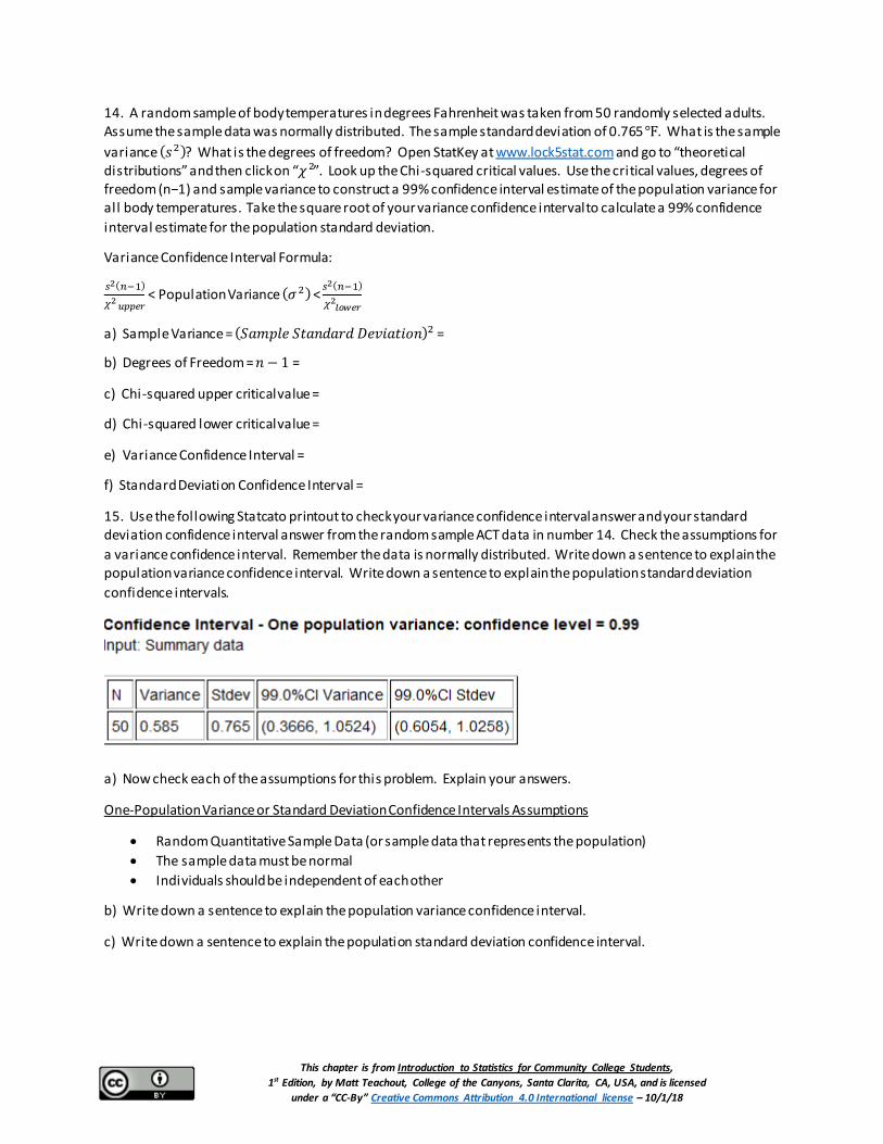
This chapter is from Introduction to Statistics for Community College Students, 1st Edition, by Matt Teachout, College of the Canyons, Santa Clarita, CA, USA, and is licensed
under a “CC-By” Creative Commons Attribution 4.0 International license – 10/1/18
14. A random sample of body temperatures in degrees Fahrenheit was taken from 50 randomly selected adults. Assume the sample data was normally distributed. The sample standard deviation of 0.765 ℉. What is the sample variance (𝑠𝑠2)? What is the degrees of freedom? Open StatKey at www.lock5stat.com and go to “theoretical distributions” and then click on “𝜒𝜒2”. Look up the Chi-squared critical values. Use the critical values, degrees of freedom (n−1) and sample variance to construct a 99% confidence interval estimate of the population variance for all body temperatures. Take the square root of your variance confidence interval to calculate a 99% confidence interval estimate for the population standard deviation.
Variance Confidence Interval Formula:
𝐵𝐵2(𝑛𝑛−1)
𝜒𝜒 𝑢𝑢𝑢𝑢𝑢𝑢𝑢𝑢𝑢𝑢2 < Population Variance (𝜎𝜎2) < 𝐵𝐵2(𝑛𝑛−1)
𝜒𝜒 𝑙𝑙𝑙𝑙𝑙𝑙𝑢𝑢𝑢𝑢2
a) Sample Variance = (𝑆𝑆𝑆𝑆𝑆𝑆𝑝𝑝𝑆𝑆𝑆𝑆 𝑆𝑆𝑆𝑆𝑆𝑆𝑛𝑛𝑑𝑑𝑆𝑆𝑀𝑀𝑑𝑑 𝐷𝐷𝑆𝑆𝐷𝐷𝑆𝑆𝑆𝑆𝑆𝑆𝑆𝑆𝑜𝑜𝑛𝑛)2 =
b) Degrees of Freedom = 𝑛𝑛− 1 =
c) Chi-squared upper critical value =
d) Chi-squared lower critical value =
e) Variance Confidence Interval =
f) Standard Deviation Confidence Interval =
15. Use the following Statcato printout to check your variance confidence interval answer and your standard deviation confidence interval answer from the random sample ACT data in number 14. Check the assumptions for a variance confidence interval. Remember the data is normally distributed. Write down a sentence to explain the population variance confidence interval. Write down a sentence to explain the population standard deviation confidence intervals.
a) Now check each of the assumptions for this problem. Explain your answers.
One-Population Variance or Standard Deviation Confidence Intervals Assumptions
• Random Quantitative Sample Data (or sample data that represents the population) • The sample data must be normal • Individuals should be independent of each other
b) Write down a sentence to explain the population variance confidence interval.
c) Write down a sentence to explain the population standard deviation confidence interval.
This chapter is from Introduction to Statistics for Community College Students, 1st Edition, by Matt Teachout, College of the Canyons, Santa Clarita, CA, USA, and is licensed
under a “CC-By” Creative Commons Attribution 4.0 International license – 10/1/18
One-Population Bootstrap Confidence Interval Practice Problems
16. Go to www.lock5stat.com and click on the “StatKey” tab. Under the “Bootstrap Confidence Intervals” menu, click on “CI for Single Mean, Median, St.Dev.” Click on the left corner and change the data set to “BodyTemp50”. This data gives a random sample of the body temperatures of 50 adults in degrees Fahrenheit.
a) Create the bootstrap sampling distribution for the mean. Use the bootstrap distribution to find a 99% confidence interval for the population mean body temperature. How many samples did you take? What is the shape of the bootstrap distribution? Write the upper and lower limits of the interval below. Write a sentence to explain the confidence interval. Assuming this data was random, would this data set have met the assumptions for mean average confidence intervals that use the regular calculation with T-scores? Explain.
b) Create the bootstrap sampling distribution for the median. Use the bootstrap distribution to find a 99% confidence interval for the population median body temperature. How many samples did you take? What is the shape of the bootstrap distribution? Write the upper and lower limits of the interval below. Write a sentence to explain the confidence interval.
c) Create the bootstrap sampling distribution for the standard deviation. Use the bootstrap distribution to find a 99% confidence interval for the population standard deviation for body temperature. How many samples did you take? What is the shape of the bootstrap distribution? Write the upper and lower l imits of the interval below. Write a sentence to explain the confidence interval.
17. Go to www.lock5stat.com and click on the “StatKey” tab. Under the “Bootstrap Confidence Intervals” menu, click on “CI for Single Mean, Median, St.Dev.” Click on the left corner and change the data set to “Florida Lakes (pH)”. This data gives the pH from 53 randomly selected lakes in Florida.
a) Create the bootstrap sampling distribution for the mean. Use the bootstrap distribution to find a 90% confidence interval to estimate the population mean pH in all Florida lakes. How many samples did you take? What is the shape of the bootstrap distribution? Write the upper and lower limits of the interval below. Write a sentence to explain the confidence interval. Assuming this data was random, would this data set have met the assumptions for mean average confidence intervals that use the regular calculation with T-scores? Explain.
b) Create the bootstrap sampling distribution for the median. Use the bootstrap distribution to find a 90% confidence interval for the population median pH in all Florida lakes. How many samples did you take? What is the shape of the bootstrap distribution? Write the upper and lower limits of the interval below. Write a sentence to explain the confidence interval.
c) Create the bootstrap sampling distribution for the standard deviation. Use the bootstrap distribution to find a 90% confidence interval for the population standard deviation for pH in all Florida lakes. How many samples did you take? What is the shape of the bootstrap distribution? Write the upper and lower l imits of the interval below. Write a sentence to explain the confidence interval.
18. Go to www.lock5stat.com and click on the “StatKey” tab. Under the “Bootstrap Confidence Intervals” menu, click on “CI for Single Mean, Median, St.Dev.” Click on the left corner and change the data set to “Restaurant Tips”. This data gives the amount of tip for 157 bills at a restaurant.
a) Create the bootstrap sampling distribution for the mean. Use the bootstrap distribution to find a 95% confidence interval to estimate the population mean average amount of tips at the restaurant. How many samples did you take? What is the shape of the bootstrap distribution? Write the upper and lower limits of the interval

This chapter is from Introduction to Statistics for Community College Students, 1st Edition, by Matt Teachout, College of the Canyons, Santa Clarita, CA, USA, and is licensed
under a “CC-By” Creative Commons Attribution 4.0 International license – 10/1/18
below. Write a sentence to explain the confidence interval. Assuming this data was random, would this data set have met the assumptions for mean average confidence intervals that use the regular calculation with T-scores? Explain.
b) Create the bootstrap sampling distribution for the median. Use the bootstrap distribution to find a 95% confidence interval to estimate the population median average amount of tips at the restaurant. How many samples did you take? What is the shape of the bootstrap distribution? Write the upper and lower l imits of the interval below. Write a sentence to explain the confidence interval.
c) Create the bootstrap sampling distribution for the standard deviation. Use the bootstrap distribution to find a 95% confidence interval to estimate the population standard deviation of tips at the restaurant. How many samples did you take? What is the shape of the bootstrap distribution? Write the upper and lower l imits of the interval below. Write a sentence to explain the confidence interval.
19. Go to www.lock5stat.com and click on the “StatKey” tab. Under the “Bootstrap Confidence Intervals” menu, click on “CI for Single Proportion”. Click on the left corner and change the data set to “Regular Exercise Important? (US adults)”. A 1000 randomly selected Americans were asked if they believe regular exercise is important.
Create the bootstrap sampling distribution for the proportion. Use the bootstrap distribution to find a 99% confidence interval to estimate the population proportion (percent) of all Americans that think regular exercise is important. How many samples did you take? What is the shape of the bootstrap distribution? Write the upper and lower limits of the interval below in both decimal form and as percentages. Write a sentence to explain the confidence interval. Assuming this data was random, would this data set have met the assumptions for proportion confidence intervals that use the regular calculation with Z-scores? Explain.
20. Go to www.lock5stat.com and click on the “StatKey” tab. Under the “Bootstrap Confidence Intervals” menu, click on “CI for Single Proportion”. Click on the left corner and change the data set to “Lie Detector (Missed a lie)”. Giving lie detector tests are not easy and the people giving the test can make mistakes. A random sample of 48 l ie detector tests were reviewed for errors, specifically if the tester did not catch when a person lied. They found that in 17 of the 48 tests, the tester did not catch at least one of the l ies.
Create the bootstrap sampling distribution for the proportion. Use the bootstrap distribution to find a 90% confidence interval to estimate the population proportion (percent) of all l ie detector tests that fail to catch at least one l ie. How many samples did you take? What is the shape of the bootstrap distribution? Write the upper and lower limits of the interval below in both decimal form and as percentages. Write a sentence to explain the confidence interval. Assuming this data was random, would this data set have met the assumptions for proportion confidence intervals that use the regular calculation with Z-scores? Explain.
This chapter is from Introduction to Statistics for Community College Students, 1st Edition, by Matt Teachout, College of the Canyons, Santa Clarita, CA, USA, and is licensed
under a “CC-By” Creative Commons Attribution 4.0 International license – 10/1/18
21. Go to www.lock5stat.com and click on the “StatKey” tab. Under the “Bootstrap Confidence Intervals” menu, click on “CI for Single Proportion”. Click on the left corner and change the data set to “Know Hear Attack Symptom (Europeans)”. A random sample of 10228 Europeans were asked if they knew the symptoms of a heart attack. Only 4910 of them did know all of the correct symptoms of a heart attack.
Create the bootstrap sampling distribution for the proportion. Use the bootstrap distribution to find a 95% confidence interval to estimate the population proportion (percent) of all Europeans that know the correct symptoms of a heart attack. How many samples did you take? What is the shape of the bootstrap distribution? Write the upper and lower l imits of the interval below in both decimal form and as percentages. Write a sentence to explain the confidence interval. Assuming this data was random, would this data set have met the assumptions for proportion confidence intervals that use the regular calculation with Z-scores? Explain.
--------------------------------------------------------------------------------------------------------------------------------------------------------
Section 3F – Two-Population Confidence Intervals