52

Chapter 3

Analytical Prediction Methods

Analytical predictions of modal properties and acceleration response to walking

were performed for the six floors described in Chapter 2. The objective was to obtain

predictions that could be compared to the measurements to judge the accuracy of the

analytical methods. This chapter describes the analytical prediction methods and Chapter

4 contains the comparisons. Note that “design” analytical methods are defined in Chapter

5.

Modal properties and accelerance FRF magnitudes were predicted using standard

eigenvalue analyses and steady-state analyses, respectively. Accelerations due to

walking were predicted using the three different methods that were briefly described in

Chapter 1: response history using individual footstep forces, response history using

Fourier series loading, and a simplified frequency domain analysis method.

3.1 Modeling and Prediction of Modal Properties Reasonable prediction of modal properties (natural frequencies, mode shapes, and

damping) is the essential first step toward a reasonable prediction of acceleration due to

walking. This step involves two activities: definition of the structure and eigenvalue

analysis to predict the natural frequencies and mode shapes. Defining the structure is

straightforward in most respects. Succinctly, this entails creating a finite element model

with geometry, mass, and stiffness approximating those of the real structure. With the

structure defined, well known methods are used to compute the natural frequencies and

mode shapes. Damping cannot be directly computed, so measured values are used.

3.1.1 Defining the Structure

The structures were defined using a combination of the methods given in DG11,

Barrett (2006), and the SCI DG.

Slab Shell Elements The floor slabs were modeled using SAP2000 (CSi 2005) thin shell elements

based on the Kirchhoff formulation. As was reported by Barrett (2006), use of the

53

thicker plate (Mindlin / Reissner formulation) resulted in slightly higher frequencies: up

to 6% higher for the long span composite slab specimens and 1% higher for the other

specimens. Shell elements were used, rather than the plate elements, because their in-

plane degrees of freedom restrain weak-axis beam bending. Otherwise, weak-axis beam

bending mode shapes could be predicted in the frequency bandwidth under consideration.

The deck-supported slabs studied in this research were all significantly

orthotropic, with ratios of strong- to weak-direction stiffness ranging from 1.5 to 2.7.

Shell elements were made orthotropic using area element flexural stiffness property

modifiers. In each case, the concrete elastic modulus was computed using the dynamic

elastic modulus recommended in DG11, that is, 1.35 times the static elastic modulus.

Concrete elastic moduli were computed using measured concrete unit weights and

strengths for the laboratory specimens, but nominal properties were used for the others.

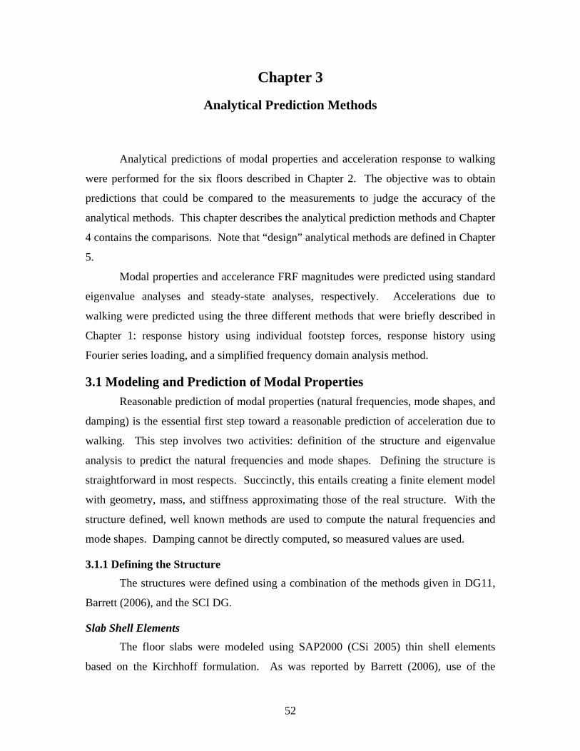
Visible cracks were seen at supports at the Shear-Connected Joist Footbridge,

Riverside MOB, and Composite Slab Mockup. However, no established procedure exists

for considering the effects of these cracks. It is likely that they have some effect on

modes that have significant curvature at the supports. For example, the measured mode

shown in Figure 3.1(a) has little curvature at the support between the two bays with

significant displacement, so cracking should have little effect on this mode; whereas, the

mode shown in Figure 3.1(b) has much more significant curvature at the support. The

predictions in Chapter 4 were made using no modification in the shell elements to

account for cracking. The effect of cracking is revisited in Chapter 5.

Figure 3.1: Sample Mode Shapes. (a) Little or No Curvature at Support; (b)

Significant Curvature at Support.

54

Shells were automatically submeshed into elements of approximately 24 in. to 36

in. The natural frequencies converged within 1% at a 36 in. size, so that was considered

to be a reasonable maximum element size for bays included in this research. Elements

were usually rectangular with exceptions being at elements with nodes that were moved

slightly to footstep locations. Beam and girders were automatically subdivided to ensure

that their nodes coincided with the shell nodes.

Steel Members

For all but two specimens, beams and girders were modeled using frame elements

in the same plane as the shell elements. Transformed strong-axis moments of inertia

were computed as recommended in DG11. For the joist footbridges, the frame elements

were bare steel and offset below the shell elements by the distance between the top chord

centroid and the centroid of the solid portion of the slab. The shell elements and top

chord frame elements were connected using vertical rigid links between nodes. In all

cases, the beam and girder ends were continuously connected regardless of the type of

connection that existed in reality. This is consistent with finite element modeling

recommendations of the SCI DG and is reasonable because floor vibration due to human

walking results in forces that are insufficient to cause bolt slip or significant deformation

at shear connections. Where applicable, the columns were included in the model and

extended to halfway below and above the floor being modeled. This is also consistent

with the finite element modeling recommendations of the SCI DG. The assumption is

that the mode shapes will have the columns in double curvature, so halfway below and

above the floor are inflection points. Spandrel members at cladding were assumed to be

2.5 times stiffer than computed, per the recommendations of Barrett (2006).

Masses

Masses were assigned using three different equivalent methods for the various

models. In the first method, the “Vibecon” material property (Barrett 2006) was used. In

short, the concrete, deck, and superimposed masses are combined and used to create a

fictitious concrete density (kip sec.2 / in. / in.3) that will result in the correct area mass. In

the second method, the area masses are computed separately and assigned to the shells in

the model. The material density is set to zero to avoid double counting the mass. The

55

last option is to apply the mass as loads (in the very familiar units of psf, for example) in

the model and then define the “Mass Source” as being “From Element and Additional

Masses and Loads,” with the material density set to zero. This last method has the

advantage of being quickly verified at a later date because the force/area units are very

commonly used. In all three methods, the steel member masses are computed by

SAP2000. Because the specimens were bare slabs, the area masses were simply the best

estimates of the slab and deck masses. Spandrel masses were applied as line masses

where applicable.

3.1.2 Prediction of Natural Frequencies and Mode Shapes Natural frequencies and mode shapes were predicted by solving the multi degree

of freedom (MDOF) undamped free vibration eigenvalue problem which is described in

detail in vibrations textbooks (Clough and Penzien 1993, Ewins 2000, Chopra 2001).

The eigenvalue problem solution is valid for undamped and proportionally damped

systems. As seen in Chapter 4, the measured vibration modes for the floor structures

included in this research were mostly quasi-real, so the assumption of proportional

damping is acceptable. Another option is to use Ritz-vector analysis rather than

eigenvalue analysis. Barrett (2006) reported that Ritz-vector analysis provided no

advantage over eigenvalue analysis for planar floors such as the ones included in this

research and actually results in illogical higher mode predictions in some cases.

Therefore, eigenvalue analysis was used throughout this research. Sample predicted

mode shapes are shown in Figure 3.2. These first nine modes are in the frequency

bandwidth that can be excited by human walking. Of course, the model computed many

more modes, but their frequencies are too high to be of interest.

The number of modes was selected so that the highest modal frequency was

approximately 15 Hz. The resulting analysis bandwidth (0-15 Hz) approximately

matches the bandpass filter limits that were used during post-processing of the

measurements (1-15 Hz) and is reasonable in general for low frequency floors (natural

frequencies under approximately 10 Hz). The higher frequency modes in a low

frequency floor are inevitably double curvature in some or all bays, so have little effect

on the acceleration at midspan. Also, as shown in Chapter 4, finite element modeling can

only predict mode shapes to a moderate degree of accuracy. It is very unlikely that the

56

analysis procedure will accurately predict these higher frequency modes, so terminating

the analysis at 15 Hz is reasonable.

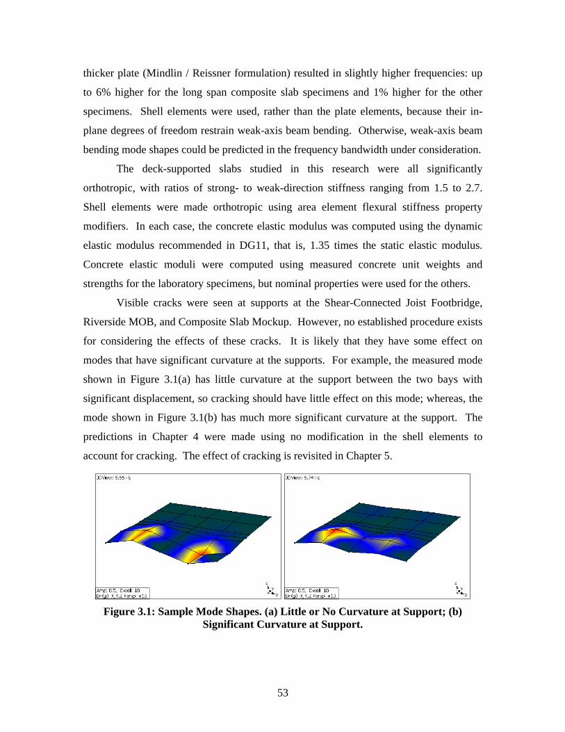
Natural frequencies and mode shapes are only the first step toward the actual

goal: prediction of acceleration response to human walking. As can be seen from Figure

3.2, numerous modes are predicted. It is usually somewhat difficult, and sometimes

impossible, to determine which mode or modes will be responsive in a given bay simply

by looking at the mode shapes.

Figure 3.2: Sample Computed Mode Shapes (Riverside MOB). (a) Mode 1: 6.50 Hz; (b) Mode 2: 6.93 Hz; (c) Mode 3: 7.12 Hz; (d) Mode 4: 7.34 Hz; (e) Mode 5: 7.45 Hz; (f) Mode 6: 7.51 Hz; (g) Mode 7: 7.88 Hz; (h) Mode 8: 7.94 Hz; (i) Mode 9: 8.20 Hz.

3.1.3 Damping Damping of structures in service is provided almost entirely by non-structural

elements which were not present during the experimental program. DG11 and the SCI

DG recommend bare slab critical viscous damping ratios of 1.0% and 1.1%, respectively.

Measured damping values for the tested bare slabs were found to vary between 0.17% of

critical and 1.5% of critical even though they were all bare slabs. Therefore, to create

57

reasonable comparisons, measured critical damping ratios were used in all of the

acceleration predictions.

3.2 Accelerance FRF Magnitude Prediction

Natural frequencies and mode shapes provide important information about the

structure, but as mentioned previously, it is often difficult to determine which modes are

significant in a bay if only the natural frequencies and mode shapes are known.

Predictions of FRF magnitudes were used to determine which modes would be

responsive in a given bay. SAP2000 provides a very convenient feature to compute and

display the FRF: Steady-State Analysis. The analysis method is described in detail by

Barrett (2006). In summary, the system equations of motion, with the loading function

having a cosine and a sine term, are solved using direct integration at each specified

spectral line. The resulting response is composed of a real and an imaginary part at each

spectral line, both of which are analogous to the corresponding measured values. The

magnitude of this complex number at each line is the FRF magnitude. (The phase can be

obtained also, but is not of interest for this research.) The frequency bandwidths were

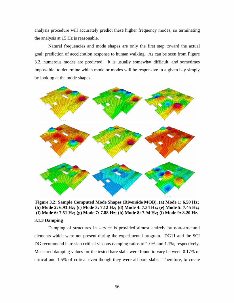
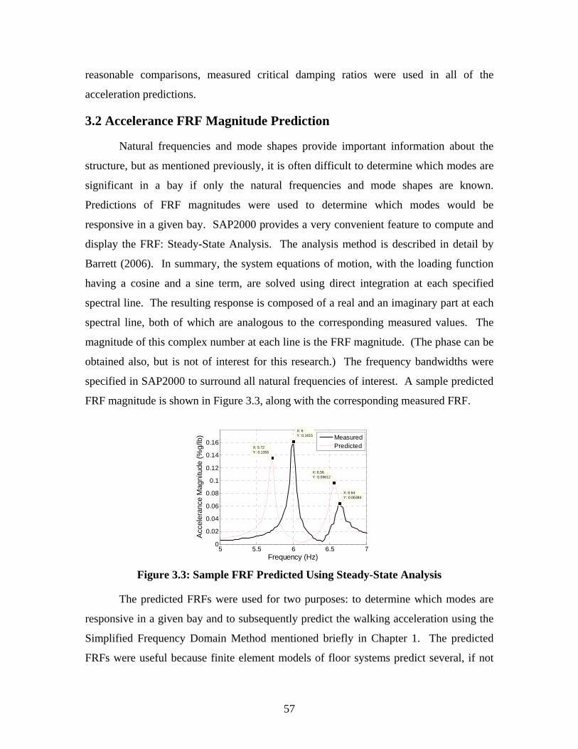
specified in SAP2000 to surround all natural frequencies of interest. A sample predicted

FRF magnitude is shown in Figure 3.3, along with the corresponding measured FRF.

5 5.5 6 6.5 70

0.02

0.04

0.06

0.08

0.1

0.12

0.14

0.16

Frequency (Hz)

Acc

eler

ance

Mag

nitu

de (%

g/lb

)

X: 6Y: 0.1615

X: 5.72Y: 0.1355

X: 6.56Y: 0.09612

X: 6.64Y: 0.06384

MeasuredPredicted

Figure 3.3: Sample FRF Predicted Using Steady-State Analysis

The predicted FRFs were used for two purposes: to determine which modes are

responsive in a given bay and to subsequently predict the walking acceleration using the

Simplified Frequency Domain Method mentioned briefly in Chapter 1. The predicted

FRFs were useful because finite element models of floor systems predict several, if not

58

dozens, of vibration modes. The FRF magnitude plot in each bay allowed immediate

judgment of which modes would be highly responsive if excited. (Response history

analysis for a unit load at each modal frequency also allows one to plot the FRF line-by-

line, but this is far less convenient than using steady-state analysis.)

Because all measurements were taken with the shaker at mid-bay, the load was

also applied there in the models. Any type of load or combination of loads can be used as

the “input” for this type of frequency domain analysis, but a single 1 lbf point load at

mid-bay was used in all cases. The FRFs were computed for all degrees of freedom in

the model, but the mid-bay (driving point) FRFs are of primary interest for this research

because they can be compared directly to measurements and because that location serves

as the assumed loading point for the Simplified Frequency Domain Analysis procedure.

The measured FRFs are scaled to display the accelerance in the most intuitive units:

%g/lbf. Therefore, the predicted accelerances are also scaled to this unit by multiplying

the acceleration (in./sec.2) by 100/386 = 0.2591 to obtain %g/lbf units.

SAP2000’s steady-state analysis requires the use of hysteretic damping instead of

viscous damping. However, all of the measured critical damping ratios were obtained in

the form of viscous damping. As described in Ewins (2000), Chopra (2001), and the

SAP2000 User’s Manual (CSi 2005), the response is equivalently computed at natural

frequencies using hysteretic damping equal to double the viscous damping ratio. For

example, if the viscous damping ratio is 0.005 at a natural mode, a hysteretic damping

ratio of 0.01 results in an equivalent acceleration response at that modal frequency.

SAP2000 allows these damping ratios to be input as constant for all frequencies or

different at specified frequencies and interpolated in-between. Whenever possible,

measured damping ratios were selected to match each responsive frequency in the bay

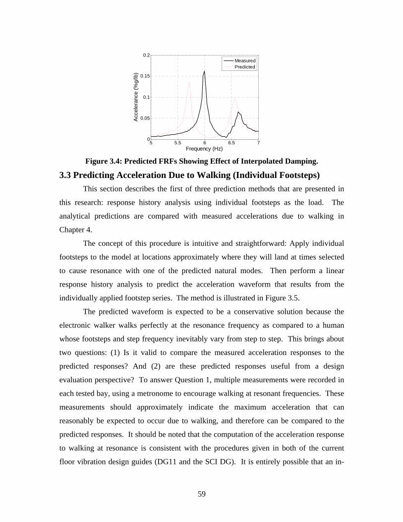
containing the driving point. For example, the predicted FRF in Figure 3.4 was

computed using hysteretic damping selected to match the first and second modal damping

ratios. If constant hysteretic damping had been used, equal to the measured first modal

damping ratio, the second mode’s peak would have been much taller and narrow, causing

a less accurate prediction.

59

5 5.5 6 6.5 70

0.05

0.1

0.15

0.2

Frequency (Hz)

Acc

eler

ance

(%g/

lb)

MeasuredPredicted

Figure 3.4: Predicted FRFs Showing Effect of Interpolated Damping.

3.3 Predicting Acceleration Due to Walking (Individual Footsteps) This section describes the first of three prediction methods that are presented in

this research: response history analysis using individual footsteps as the load. The

analytical predictions are compared with measured accelerations due to walking in

Chapter 4.

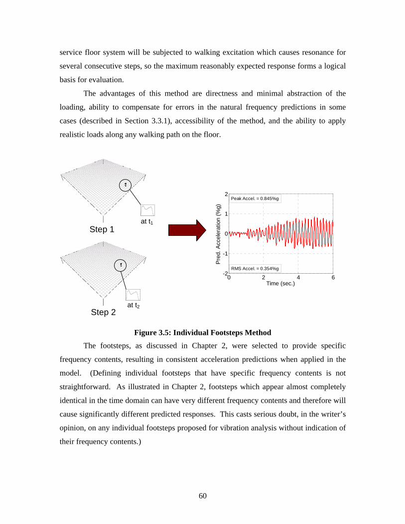
The concept of this procedure is intuitive and straightforward: Apply individual

footsteps to the model at locations approximately where they will land at times selected

to cause resonance with one of the predicted natural modes. Then perform a linear

response history analysis to predict the acceleration waveform that results from the

individually applied footstep series. The method is illustrated in Figure 3.5.

The predicted waveform is expected to be a conservative solution because the

electronic walker walks perfectly at the resonance frequency as compared to a human

whose footsteps and step frequency inevitably vary from step to step. This brings about

two questions: (1) Is it valid to compare the measured acceleration responses to the

predicted responses? And (2) are these predicted responses useful from a design

evaluation perspective? To answer Question 1, multiple measurements were recorded in

each tested bay, using a metronome to encourage walking at resonant frequencies. These

measurements should approximately indicate the maximum acceleration that can

reasonably be expected to occur due to walking, and therefore can be compared to the

predicted responses. It should be noted that the computation of the acceleration response

to walking at resonance is consistent with the procedures given in both of the current

floor vibration design guides (DG11 and the SCI DG). It is entirely possible that an in-

60

service floor system will be subjected to walking excitation which causes resonance for

several consecutive steps, so the maximum reasonably expected response forms a logical

basis for evaluation.

The advantages of this method are directness and minimal abstraction of the

loading, ability to compensate for errors in the natural frequency predictions in some

cases (described in Section 3.3.1), accessibility of the method, and the ability to apply

realistic loads along any walking path on the floor.

Figure 3.5: Individual Footsteps Method The footsteps, as discussed in Chapter 2, were selected to provide specific

frequency contents, resulting in consistent acceleration predictions when applied in the

model. (Defining individual footsteps that have specific frequency contents is not

straightforward. As illustrated in Chapter 2, footsteps which appear almost completely

identical in the time domain can have very different frequency contents and therefore will

cause significantly different predicted responses. This casts serious doubt, in the writer’s

opinion, on any individual footsteps proposed for vibration analysis without indication of

their frequency contents.)

Step 1

Step 2

0 0 .1 0 .2 0.3 0.4 0.5 0 .6 0 .7 0 .80

0.0 5

0 .1

0.1 5

0 .2

0.2 5

0 0 .1 0 .2 0 .3 0 .4 0 .5 0 .6 0 .7 0 .80

0.0 5

0 .1

0.1 5

0 .2

0.2 5

at t1

at t2

0 2 4 6-2

-1

0

1

2

Time (sec.)

Pre

d. A

ccel

erat

ion

(%g)

Peak Accel. = 0.845%g

RMS Accel. = 0.354%g

61

The method can also be implemented using several readily available structural

analysis programs and should be easily adapted to use on high frequency floors, stairs,

and other structures.

The main disadvantage is the inability to quickly set up analysis cases with

multiple footsteps. If desired, preprocessors can be created or the method can be

included in analysis programs for automatic usage. Also, in many cases, short walking

paths might only require the application of a small number of steps. A secondary

disadvantage is the necessity of having numerous footsteps to cover the realistic step

frequency range, 1.6 Hz to 2.2 Hz. As discussed in Chapter 2, it is not possible to define

one, or even a few individual design footsteps because their frequency content varies

greatly when they are applied at other step frequencies.

3.3.1 Footstep Force Application The FRF magnitude prediction allows the next step: determination of footstep

force loads that will cause resonance and therefore cause the maximum acceleration

response that can be reasonably expected for a person walking across the bay.

In each bay included in this research, the step frequency was selected to cause

resonance with a predicted mode. The considered human step frequency range is 1.6 Hz

to 2.2 Hz, which is well below the natural frequency of any acceptable floor system.

However, the series of applied footstep forces is made up of the superposition of

sinusoids with specific amplitudes and phases. The frequencies of these sinusoids are

integer multiples of the frequency of the lowest frequency sinusoid (which has a

frequency equal to the step frequency). Therefore, if a natural frequency exists at an

integer multiple of the step frequency, resonance will also occur.

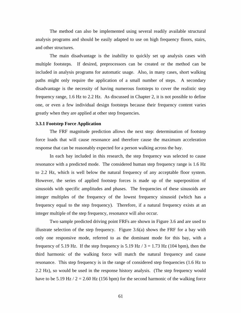
Two sample predicted driving point FRFs are shown in Figure 3.6 and are used to

illustrate selection of the step frequency. Figure 3.6(a) shows the FRF for a bay with

only one responsive mode, referred to as the dominant mode for this bay, with a

frequency of 5.19 Hz. If the step frequency is 5.19 Hz / 3 = 1.73 Hz (104 bpm), then the

third harmonic of the walking force will match the natural frequency and cause

resonance. This step frequency is in the range of considered step frequencies (1.6 Hz to

2.2 Hz), so would be used in the response history analysis. (The step frequency would

have to be 5.19 Hz / 2 = 2.60 Hz (156 bpm) for the second harmonic of the walking force

62

to cause resonance, but this frequency is well outside the considered step frequency range

so would not be used to define the loads. The step frequency would have to be 1.29 Hz

(78 bpm) for the fourth harmonic to match the natural frequency and cause resonance.)

The walking force decreases for higher harmonics, so the lowest harmonic that falls

within the considered step frequency range should always used. Figure 3.6(b) shows the

FRF for a bay with three responsive modes in the frequency range that can be excited by

human walking. In this case, excitation of the 7.12 Hz mode using the fourth harmonic

of the walking force, step frequency = 7.12 Hz / 4 = 1.78 Hz (107 bpm), would be used to

define the walking force. It is unknown whether excitation of the 7.34 Hz mode would

cause higher response, so a separate load case could be defined for it also. It may not be

possible to simply use one analysis case exciting the mode with the highest accelerance

peak magnitude (dominant mode) because the goal is to predict the maximum

acceleration due to walking.

4 4.5 5 5.5 60

0.1

0.2

0.3

0.4X: 5.187Y: 0.3806

Frequency (Hz)

Acc

eler

ance

Mag

nitu

de (%

g/lb

f)

6 7 8 90

0.05

0.1

0.15 X: 7.336Y: 0.1377

Frequency (Hz)

Acc

eler

ance

Mag

nitu

de (%

g/lb

f) X: 7.124Y: 0.1528

X: 8.2Y: 0.07519

Figure 3.6: Sample Predicted FRFs; (a) One Dominant Mode; (b) Three Responsive

Modes

Exciting the floor system at resonance, rather than applying footsteps at natural

step frequencies has the advantage of compensating for inaccurate natural frequency

prediction, assuming that the accelerance peak magnitude is reasonably well predicted.

For example, consider a floor with a natural frequency of 6.0 Hz and acceleration peak

magnitude of 0.2 %g/lbf. The maximum response will occur due to walking at 6.0 Hz / 3

= 2.0 Hz (120 bpm), with the walking force third harmonic causing resonance. If the

model predicted a natural frequency of 6.5 Hz and an accelerance peak magnitude

approximately 0.2 %g/lbf, then the acceleration due to walking will still be accurately

63

predicted. The electronic walker’s step frequency would be 6.5 Hz / 3 = 2.17 Hz (130

bpm) in the model, causing resonance with the walking force third harmonic. The third

harmonic amplitudes for walking at 2.0 Hz and 2.17 Hz are not appreciably different,

especially compared to the overall scatter of footstep force harmonic amplitudes. On the

other hand, if the analysis procedure used “natural” or “normal” walking frequencies,

which are approximately 2.0 Hz, the response would have been very significantly under-

predicted. In this prediction, the excitation would be applied off-resonance whereas it

would be likely to excite the actual structure at resonance. Granted, it is usually easier to

accurately predict the natural frequency than the accelerance peak magnitude, but

applying forces to cause resonance at least compensates for one potential error source.

There are several comparisons of measured and predicted FRFs in Chapter 4 which have

better predictions of FRF peak magnitude than natural frequency. Consider also that a

5% error in FRF estimate will result in approximately a 5% error in prediction of

acceleration due to walking. On the other hand, the predicted response varies very

significantly if the step frequency is applied very close to a resonant frequency or at a

frequency just slightly off-resonance.

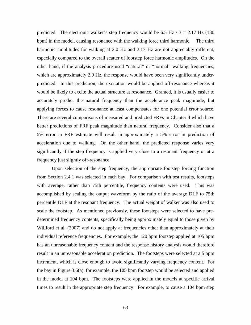
Upon selection of the step frequency, the appropriate footstep forcing function

from Section 2.4.1 was selected in each bay. For comparison with test results, footsteps

with average, rather than 75th percentile, frequency contents were used. This was

accomplished by scaling the output waveform by the ratio of the average DLF to 75th

percentile DLF at the resonant frequency. The actual weight of walker was also used to

scale the footstep. As mentioned previously, these footsteps were selected to have pre-

determined frequency contents, specifically being approximately equal to those given by

Willford et al. (2007) and do not apply at frequencies other than approximately at their

individual reference frequencies. For example, the 120 bpm footstep applied at 105 bpm

has an unreasonable frequency content and the response history analysis would therefore

result in an unreasonable acceleration prediction. The footsteps were selected at a 5 bpm

increment, which is close enough to avoid significantly varying frequency content. For

the bay in Figure 3.6(a), for example, the 105 bpm footstep would be selected and applied

in the model at 104 bpm. The footsteps were applied in the models at specific arrival

times to result in the appropriate step frequency. For example, to cause a 104 bpm step

64

frequency, steps would be applied in the model at 0.5769 sec. increments (0 sec., 0.5769

sec., 1.1538 sec., etc.).

Footsteps were applied in the model to nodes at approximate footstep locations.

In a design setting, footstep locations will not be known, so they would be spaced equally

at approximately the average human stride length. Human stride lengths vary depending

on step frequency, but the mean is approximately 26-30 in., (Pachi and Ji 2005,

Zivanovic et al. 2006). Observed stride lengths during the experimental program fell into

this stride range. Often, nodes do not exist in the model at approximately this spacing.

Three options exist for situations such as this: further subdivide the shells to provide

nodes at approximately the required locations, use a coarser mesh and individually move

specific nodes to appropriate locations, or use line elements between nodes and apply the

load as a member load instead. In this research, the shells were either further subdivided

or specific nodes were moved to provide nodes in the desired locations.

Small step location discrepancies are not considered by the writer to be significant

because the acceleration response at midspan should not be significantly different due to

a footstep landing at one location or a foot or two away . To understand why this is true,

consider the form of the multi-degree of freedom frequency response function (Ewins

2000).

( ) ∑= ωωζ+ω+ω−

φ⋅φω=

R

1r rrr2r

2krir2

k

i

M)2j(j

fx&&

Eq. 3.1

where

ix&& = Acceleration at spatial location (DOF), i

kf = Forcing function at spatial location (DOF), k r = Mode index R = Number of modes

ir φ = rth mode vector amplitude at location i

kr φ = rth mode vector amplitude at location k ω = Forcing frequency (angular)

rω = rth natural frequency (angular)

rζ = Damping ratio of the rth mode Mr = Modal mass of the rth mode

65

For the rth mode’s contribution to the acceleration response at a given location, i,

all parameters on the right side of Eq. 3.1 are identical regardless of force location except

for kr φ , the mode vector location at the forcing function. Given that most floor vibration

mode shapes approximately form a sine wave, the mode vector amplitude at location kr φ

is practically identical to the mode vector amplitude a short distance away. Therefore,

the acceleration response will be practically identical if the footstep is applied at location

k, or a short distance from location k.

3.3.2 Response History Analysis With the model defined and footstep forces applied, response history (time

history) analysis was used to predict the acceleration waveform. The following aspects

of response history analysis warrant discussion: choice of solution method, time step size,

number of modes to include, and damping.

Solution Method

SAP2000 (CSi 2005) provides two types of response history analysis which

should produce the same results under ideal circumstances: Modal Superposition and

Direct Integration. Modal Superposition entails decoupling the system equations of

motion, solving the uncoupled equations, and re-coupling, which requires computation of

the natural frequencies and mode shapes, which allows the user control over which

modes are included in the response history analysis. This procedure serves as a low pass

filter, excluding frequency content above the frequency of the highest computed mode.

SAP2000 can also perform direct integration of the coupled equations of motion, but this

is generally slower and offers no control over which modes are considered. It would be

possible to use direct integration and then low pass filter the results, but this has no

apparent advantage and is a prohibitive step for most structural designers. Therefore,

modal superposition was used in all of the analyses included in this research. Linear

analyses were used because the amplitude of load and displacement were very small

during vibration tests. Some nonlinearities undoubtedly exist even at these low

amplitudes, but their sources and effects are unknown. SAP2000 offers the option of

considering the load as a one-time event, including transient effects, or a repeated

66

periodic event with all transient effects damped out. All analyses in this research were

transient.

Loads were applied with specific “arrival times” as shown in Figure 3.7. These

arrival times were selected to cause resonance with a specific vibration mode as

described in a previous paragraph.

The time step size was selected to ensure a fine enough time domain resolution to

capture the maxima and minima that occurred during prediction of walking accelerations.

According to the SAP2000 User’s Manual (CSi 2005), one-tenth of the time period of the

highest mode is usually recommended. A larger value can sometimes be used without

loss of accuracy, especially if the higher modes provide only a small portion of the

response. For this research, 15 Hz was the maximum considered modal frequency, so

one-tenth of the associated period is 0.00667 sec. As a slight simplification, 0.005 sec.

was used for each analysis. (It was verified that this increment was fine enough to avoid

missed peaks in the waveforms.) A slightly larger increment could be used, but the

response history analyses using linear modal superposition are very computationally

efficient, so little analysis time would be saved. The number of output time steps was

selected to simply provide a long enough record for the electronic walker to traverse the

walking path. In most cases, the desired response history lasted 6 sec., so the number of

output time steps was 6 sec. / 0.005 sec. = 1200.

Figure 3.7: Load Application – Arrival Times

Measured modal viscous damping ratios were used in all analyses to create more

valid comparisons of experimental and predicted accelerations. Because linear modal

histories were used, there was no need for more sophisticated damping specifications

such as Rayleigh Proportional Damping.

67

Sample predicted acceleration waveforms are shown in Figure 3.8. These are

suitable for direct comparison with measured waveforms. Figure 3.8(a) and (b) show

third harmonic and fourth harmonic resonant build-ups, respectively. The third harmonic

build-up shows the distinctive repeating pattern of one minimum with an increased

amplitude followed by two minima with decreased amplitude. The pattern is similar for

the fourth harmonic build-up, except with three cycles with decreasing amplitude.

Because the electronic walker has the same footstep force at each step and walks at a

perfect cadence, the waveforms show “clean” build-ups as shown here. It was expected

that predicted waveforms will usually over-predict the acceleration because human

walkers do not walk at perfect cadences.

0 2 4 6-2

-1

0

1

2

Time (sec.)

Pre

d. A

ccel

erat

ion

(%g)

Peak Accel. = 1.18%g

RMS Accel. = 0.472%g

0 2 4 6-4

-2

0

2

4

Time (sec.)

Pre

d. A

ccel

erat

ion

(%g)

Peak Accel. = 3.68%g

RMS Accel. = 1.37%g

Figure 3.8: Sample Predicted Acceleration Waveforms. (a) Third Harmonic

Resonant Build-Up; (b) Fourth Harmonic Resonant Build-Up.

3.4 Predicting Acceleration Due to Walking (Fourier Series) This section describes the second of three prediction methods that are presented in

this research: Response history analysis using a Fourier series representation of the load.

The analytical predictions are compared with measured accelerations due to walking in

Chapter 4.

In this procedure, the load is idealized as a Fourier series and is applied at

midspan. One term of the Fourier series matches a natural frequency, therefore causing

resonance and resulting in the maximum response. Linear response history analysis is

then used to predict the acceleration due to walking. In most cases, the force harmonic

matching the natural frequency causes the vast majority of the response. However, the

responses of all considered modes to all four harmonics are automatically included in the

68

overall response. This method is a bit less direct than the one described in Section 3.3,

but has the advantage of being easier to apply in some analysis programs. Because the

load is applied at resonance, this method is also expected to produce conservative

solutions for the same reasons articulated at the start of Section 3.3. It is also expected to

be more conservative than the previously described method because the load is applied at

midspan for the duration of the entire response history analysis. Predictions generated

using this method are valid for comparison with measurements and can form the basis of

an evaluation criterion, also as described in Section 3.3.

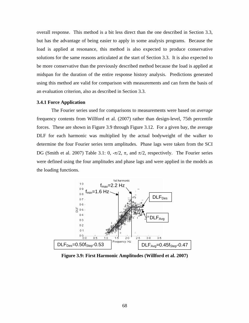
3.4.1 Force Application The Fourier series used for comparisons to measurements were based on average

frequency contents from Willford et al. (2007) rather than design-level, 75th percentile

forces. These are shown in Figure 3.9 through Figure 3.12. For a given bay, the average

DLF for each harmonic was multiplied by the actual bodyweight of the walker to

determine the four Fourier series term amplitudes. Phase lags were taken from the SCI

DG (Smith et al. 2007) Table 3.1: 0, -π/2, π, and π/2, respectively. The Fourier series

were defined using the four amplitudes and phase lags and were applied in the models as

the loading functions.

Figure 3.9: First Harmonic Amplitudes (Willford et al. 2007)

fmin=1.6 Hz fmax=2.2 Hz

DLFAvg

DLFDes

DLFAvg=0.45fStep-0.47 DLFDes=0.50fStep-0.53

69

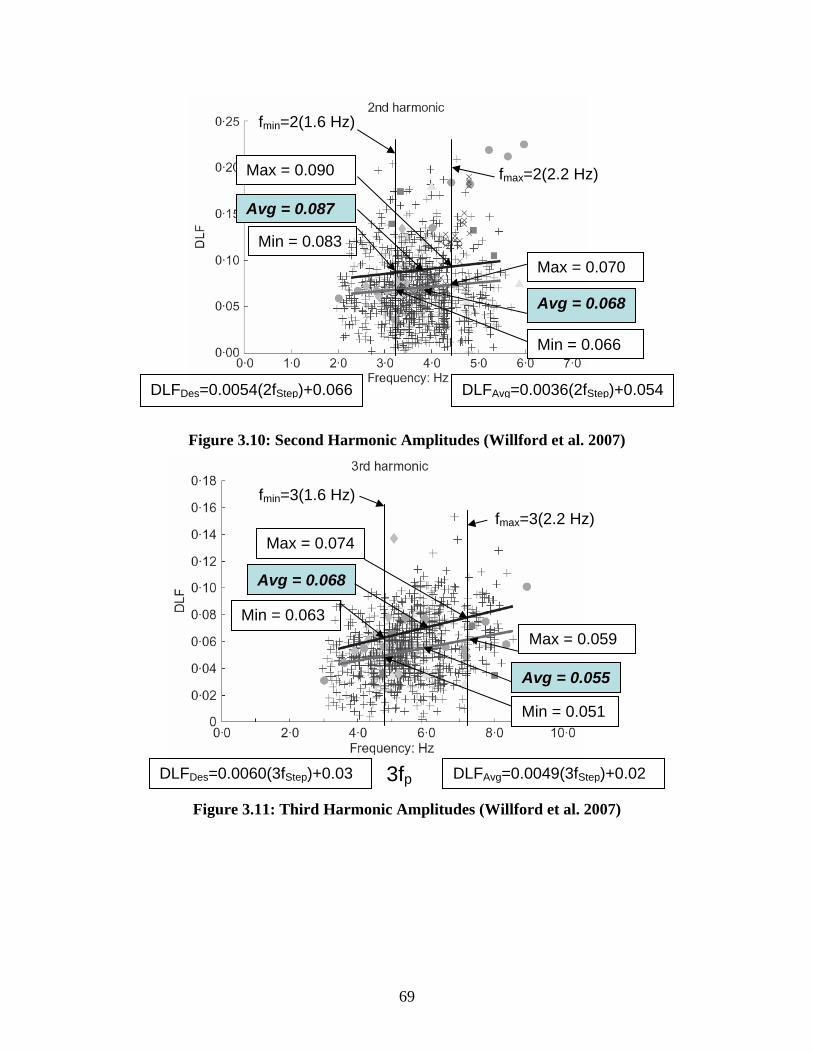
Figure 3.10: Second Harmonic Amplitudes (Willford et al. 2007)

Figure 3.11: Third Harmonic Amplitudes (Willford et al. 2007)

fmin=2(1.6 Hz)

fmax=2(2.2 Hz)

Avg = 0.087

Min = 0.083

Max = 0.090

Avg = 0.068

Max = 0.070

Min = 0.066

DLFDes=0.0054(2fStep)+0.066 DLFAvg=0.0036(2fStep)+0.054

fmin=3(1.6 Hz) fmax=3(2.2 Hz)

Avg = 0.068

Max = 0.074

Min = 0.063

Avg = 0.055

Max = 0.059

Min = 0.051

DLFDes=0.0060(3fStep)+0.03 DLFAvg=0.0049(3fStep)+0.023fp

70

Figure 3.12: Fourth Harmonic Amplitudes (Willford et al. 2007)

The Fourier series for a given bay was determined by observing which harmonic

could match the natural frequency to be excited and then determine the frequency

content. In this regard, the method is the same as the one described in Section 3.3. For

example, if the natural frequency was 5.0 Hz, the step frequency (first harmonic

frequency) would be 5.0 Hz / 3 = 1.67 Hz (100 bpm). The second through fourth

harmonic frequencies would be 3.34 Hz, 5.00 Hz, and 6.67 Hz. The average DLFs for

this series would be 0.28, 0.066, 0.045, and 0.043. If the walker weighed 150 lbf, then

the four Fourier series terms would have amplitudes equal to 42 lbf, 9.9 lbf, 6.8 lbf, and

6.5 lbf. The four sinusoidal terms would be offset relative to each other by the phase

angles listed previously in this section.

3.4.2 Response History Analysis Response history analyses were performed for each bay using the same

methodologies as described in Section 3.3.2, except for the determination of the number

of output time steps.

The number of output time steps was selected to terminate the analysis at the time

required to walk across the specimen. This was determined as follows. The number of

steps required to traverse the specimen was estimated to be the path length divided by 30

in. which is approximately the average stride length. The time required for one step was,

fmin=4(1.6 Hz) fmax=4(2.2 Hz)

Avg DLF = 0.060

Max DLF = 0.068

Min DLF = 0.052

Avg. DLF = 0.048

Max DLF = 0.054

Min DLF = 0.042

DLFAvg=0.0051(4fStep)+0.009DLFDes=0.0066(4fStep)+0.01

71

of course, the reciprocal of the step frequency. Multiplying the number of steps by the

time required for one step gave the desired duration of the response history.

This approach is a bit more direct and more accurate than the method used in the

SCI DG (Smith et al. 2007) in which the acceleration response at steady state is first

determined and then reduced to account for imperfect resonant build-up. The SCI DG

uses the resonance build-up factor shown in Eq. 3.2. (The current printing of the SCI DG

incorrectly excludes h which represents the harmonic of walking.) v/Lhf2 ppe1 ζπρ −−= Eq. 3.2

where

h = Harmonic of walking. pf = Step frequency, Hz ζ = Critical damping ratio Lp = Walking path length v = Walking speed

The resonant build-up factor is directly derived from a SDOF spring-mass-damper

system excited at resonance. The displacement response of such a system is bound by the

envelope function shown in Eq. 3.3 (Clough and Penzien 1993, Chopra 2001). Eq. 3.2

results after taking two time derivatives of the overall response equation, substituting

phf2π for ω (because h·fp matches the natural frequency), and substituting Lp / v for t.

( )1e21 t

ntDisplaceme −= −ζω

ζρ Eq. 3.3

where

ω = Excitation frequency, rad./sec.

Of course, the build-up factor only applies when the forcing frequency exactly

matches the natural frequency, which only occurs for one of the four harmonics.

However, the vast majority of the response will be from the harmonic matching

resonance, so the errors associated with this approach are small.

Measured critical damping ratios were used in all of the analysis.

Sample predicted waveforms are shown in Figure 3.13, which are both from the

same bay in the same specimen. The step frequency was equal to the third sub-harmonic

72

of the dominant frequency. Because it was expected that the response from the harmonic

matching the natural frequency will contribute the vast majority of the response, analyses

were performed using all four Fourier terms and only the term matching the natural

frequency. Figure 3.13(a) shows the waveform predicted if the Fourier series includes all

four terms and Figure 3.13(b) shows the response from only the term matching the

natural frequency. The effect of the first, second, and fourth harmonics, as seen in Figure

3.13(a), is the repeating pattern of increased amplitude followed by two decreased

amplitudes.

3.5 Predicting Acceleration Due to Walking (Simplified Frequency Domain Method)

This section describes the third of three prediction methods that are presented in

this research: The Simplified Frequency Domain Method. The analytical predictions are

compared with measured accelerations due to walking in Chapter 4.

This method advantageously uses the fact that the vast majority of the response to

walking is due to the footstep force harmonic that matches the natural frequency of the

dominant mode or another responsive mode. Succinctly, the accelerance FRF peak

magnitude is predicted (using Steady-State Analysis in SAP2000 for example) and

multiplied by the Fourier series amplitude whose frequency matches the natural

frequency. This gives the steady-state response to walking which is then reduced, using a

resonance build-up factor similar to the one shown in Eq. 3.2, to predict the actual

response to walking. This method is extremely fast and efficient. It also has the

advantage of compensating for errors in natural frequency prediction, as described in

Section 3.3. Predictions using this method are expected to be on the high side for the

same reasons articulated in Section 3.3.

73

0 2 4 6-2

-1

0

1

2

Time (sec.)

Pre

d. A

ccel

erat

ion

(%g)

Peak Accel. = 1.38%g

RMS Accel. = 0.604%g

0 2 4 6-2

-1

0

1

2

Time (sec.)

Pre

d. A

ccel

erat

ion

(%g)

Peak Accel. = 1.28%g

RMS Accel. = 0.611%g

Figure 3.13: Sample Predicted Acceleration Waveforms. (a) Four Terms; (b) One

Term. The disadvantage is that the method has no straightforward way to consider

excitation of multiple modes. In the writer’s opinion, however, this does not pose a

serious question about the usefulness of the method because finite element programs

cannot reliably predict multiple modes in the correct order and at the correct frequency

spacing anyway (Pavic et al. 2007). Ironically, if the analytical procedure predicts two

modes at a spacing that can be readily excited by two harmonics (at 6 Hz and 8 Hz for

example—both can be excited by walking at 2 Hz), then the actual structure will

probably not have these two modes at this frequency spacing. If the actual structure does

have two such modes, the analytical procedure will almost certainly not predict them.

Simply relying on the procedure’s ability to come up with one correct accelerance peak

magnitude at approximately the correct natural frequency is a realistic expectation using

the current best modeling methods. (It should be noted that no prediction method,

regardless of complexity can accurately account for multiple modes if it cannot predict

their existence.) The Simplified Frequency Domain Method is meant to provide

predictions that are accurate enough for design purposes given the current state of the art

of modal property prediction. Results from the proposed method are compared to

measurements in Chapter 4 to judge its accuracy.

This method is illustrated using the predicted accelerance FRF magnitude shown

in Figure 3.14.

74

6 7 8 90

0.05

0.1

0.15

0.2

0.25

X: 7.124Y: 0.1528

Frequency (Hz)

Acc

eler

ance

Mag

nitu

de (%

g/lb

f)

X: 7.336Y: 0.1377

X: 8.125Y: 0.151

MeasuredPredicted

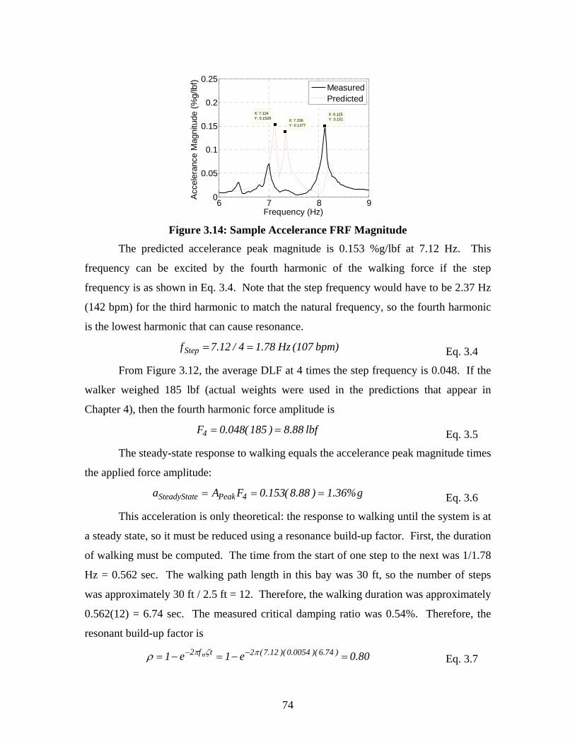
Figure 3.14: Sample Accelerance FRF Magnitude

The predicted accelerance peak magnitude is 0.153 %g/lbf at 7.12 Hz. This

frequency can be excited by the fourth harmonic of the walking force if the step

frequency is as shown in Eq. 3.4. Note that the step frequency would have to be 2.37 Hz

(142 bpm) for the third harmonic to match the natural frequency, so the fourth harmonic

is the lowest harmonic that can cause resonance.

bpm) (107Hz 78.14/12.7fStep == Eq. 3.4

From Figure 3.12, the average DLF at 4 times the step frequency is 0.048. If the

walker weighed 185 lbf (actual weights were used in the predictions that appear in

Chapter 4), then the fourth harmonic force amplitude is

lbf 88.8)185(048.0F4 == Eq. 3.5

The steady-state response to walking equals the accelerance peak magnitude times

the applied force amplitude:

g%36.1)88.8(153.0FAa 4PeakeSteadyStat === Eq. 3.6

This acceleration is only theoretical: the response to walking until the system is at

a steady state, so it must be reduced using a resonance build-up factor. First, the duration

of walking must be computed. The time from the start of one step to the next was 1/1.78

Hz = 0.562 sec. The walking path length in this bay was 30 ft, so the number of steps

was approximately 30 ft / 2.5 ft = 12. Therefore, the walking duration was approximately

0.562(12) = 6.74 sec. The measured critical damping ratio was 0.54%. Therefore, the

resonant build-up factor is

80.0e1e1 )74.6)(0054.0)(12.7(2tf2 n =−=−= −− πζπρ Eq. 3.7

75

and the acceleration due to walking in this bay is predicted to be

g%09.1)8.0(36.1aa eSteadyStatPeak ==⋅= ρ Eq. 3.8

Figure 3.14 also shows the measured accelerance magnitude. Using the peak

magnitude at 8.13 Hz, the acceleration due to walking is predicted to be 1.22 %g, which

is only 12% higher than 1.09%g which was predicted using the predicted accelerance

peak magnitude even though the measured and predicted natural frequencies were

significantly different. This is an example of the method compensating for an inaccurate

natural frequency prediction. Granted, if the accelerance peak magnitude prediction was

inaccurate, the predicted walking acceleration prediction will also be inaccurate. Again,

the accuracy of any response prediction method must rely heavily on modal properties, in

this case mode shape. If the mode shape is inaccurately predicted, then the effective

mass and accelerance peak magnitude are also inaccurately predicted.

The Simplified Frequency Domain Method also provides the opportunity to

predict the acceleration due to walking using the measured modal properties, allowing

the separation of the effects of errors in modal property predictions from errors in

walking force determination. Comparisons of measurements and predictions using

measured accelerance peak magnitudes are included in Chapter 4.