CHAPTER 3

THEORETICAL MODEL FOR THERMAL EXPANSIONAND ITS APPLICATION TO SIMPLE SYSTEMS

34

3.1 Introduction

In the first chapter, general macroscopic thcrmodynamic relations in connection

with thermal expansion were discussed. There we have seen that thermal expansion

can have contributions from various sources such as electrons, lattice, magnetic

moments and so on. We have also pointed out that these contributions can be

obtained essentially from the volume derivative of the respective entropies. We

have not however discussed so far the actual microscopic mechanisms which are

responsible for various contributions to thermal expansion. The purpose of the

present chapter is to develop a microscopic theoretical model to describe these

various contributions which will be useful to analyze the thermal expansion data.We

shall present this theoretical model in section 3.2.

As is well known, the major contribution to thermal expansion comes from the

lattice vibrations. In equilibrium, the atoms in a crystal vibrate about their mean

positions. As the temperature is raised, more and more thermal energy is injected

into the crystal and the atoms vibrate with greater and greater amplitude. Also the

mean distance of separation between the atoms increases with the increase in tem-

perature, which gives rise to the thermal expansion. Theoretically to understand

this situation one can take a potential which is a function of atomic positions. If one

takes the harmonic potential model where the positional dependence of the potential

is quadratic in the atomic displacement, there will be no lattice expansion because

of symmetrical displacements of the atoms about their equilibrium positions. Thus

vibrational thermal expansion can be obtained only from the anharmonic lattice

potential models. There have been a host of theoretical works on the vibrational

thermal expansion of solids which are based on what are known as quasi-harmonic

35

where S{hwj/k-BT) is the vibrational entroi)y function for a harmonic oscillator.

The vibrational contribution to the thermal expansion coefficient can then be cal-

culated by differentiating the entropy given by eqn.(3.1) with respect to volume.

The quasi-harmonic theory is strictly valid in the limit of small oscillations [1].

Calculations show that in hard crystals the quasi harmonic harmonic theory works

reasonably well only upto (l/6)th of the melting temperature [3]. However for soft

rare gas crystals, the quasiharmonic approach is found to fall through even at low

temperatures. In the extreme case of helium in which zero point quantum fluctu-

ations are pretty large, the quasi-harmonic approach is found to be totally invalid

at all temperatures, except at very high pressures. Thus theoretical calculations to

obtain corrections to the quasi-harmonic models due to further auharmonic effects

were called for. Various methods have indeed been suggested to deal with strongly

anharmonic crystals (see references [3-5] for review). We have recently developed

a very simple semiclassical anharmonic model for the vibrational contribution to

thermal expansion [6-8] which we shall discuss in sub-section 3.2.1.

In metals, however, in addition to phonons, free conduction electrons also con-

tribute to thermal expansion [1] which results from the volume dependence of the

models. In the quasi-harmonic theory [1,2] the vibration is still taken as harmonic

but the thermal expansion is explained by assuming volume dependent frequencies

u>}(V) where the subscript j is for different modes of vibration. In this approxima-

tion the vibrational entropy Sph is taken as a sum of contributions of various modes

and is given by

(3.1)

36

conduction electron entropy. The Somnierfeld model of non-interacting free elec-

trons suggests a linear temperature behaviour of the thermal expansion coefficient

in lowest order [1]. We shall discuss this model in sub-section 3.2.2. In magnetic

materials electron magnetic moments also contribute to thermal expansion through

their mutual interaction. At low temperatures where the effects of lattice vibrations

become very small, magnetic contributions to thermal expansion can be readily ob-

served. The magnetic contribution to thermal expansion may come from both the

itinerant and localized moments [1]. The itinerant moments contribution together

with the free electron contribution is commonly referred to as the electron-magnetic

contribution and can be described within the framework of Stoner-Wohlfarth model

[9-12] which we shall present in sub-section 3.2.3. The localized electron moments

in ferromagnetic metals and compounds would contribute to thermal expansion

through the volume dependence of the magnon entropy [1]. We shall discuss the

model for the magnon contribution to thermal expansion in sub-section 3.2.4.

In section 3.3 we apply our model to simple elemental metallic systems like Al

and Cu to examine the validity of our theoretical approach. In the next section

3.4, the thermal expansion behaviour of ferromagnetic transition metals, namely Fe

and Ni is studied within the framework of our theoretical model and the analysis of

thermal expansion data of alkali halides is then taken up and presented in section

3.5. Finally we end this chapter by giving our concluding remarks in section 3.6.

37

where (x)^ is the magnetic contribution to lattice displacement. As discussed in the

introduction, (z)™ can be written as a sum of the itinerant moment contribution

(3.5)

(3.4)

(3.3)

(3.2)

3.2 Basis of the Model

The fractional length change of a solid at any temperature T with respect or a

reference temperature To can be denned as

where a(T), the interatomic separation at temperature T, lias been written as

(x)T being the average lattice displacement at a temperature T. As alluded to in

the introduction, eqn.(3.3) can have contribution from free electrons, anharmonic

phonons, and itinerant and localized electron moments.

For a simple non-magnetic metallic system. (x)T will have contributions from

anharmonic phonons and free electrons. Hence we can write for simple metallic

systems [1]

where (x)j- is the lattice vibrational contribution and (x)eT gives the contribution

from free electrons. However for magnetic materials there will be in general addi-

tional contributions from the itinerant and localized electron moments. Thus we

can write for magnetic materials

38

where at (a,-;) is the creation (annihilation) operator for a phonon oi j — th branch

and wave vector <f and frequency u>$, $'s are related to the atomic force constant

tensors, K.m is a reciprocal lattice vector and N is the number of allowed vectors. The

(x)y and the localized moment or magnon contribution (x)™9. We shall write (x)j

and (z)'fl together as the electron-magnetic contribution {(x)™'), i.e.,

(3.6)

(3.7)

Thus (x)j for ferromagnetic materials can be finally written as

3.2.1 Theory for Vibrational Contribution

The lattice contribution to thermal expansion originates from phonon-phonon inter-

actions. These interactions arise from the anharmonic terms in an expansion of the

lattice ion-ion interaction potential energy around the equilibrium configuration of

the ions. In this anharmonic picture, a phonon has a finite life time and can decay

into other phonons through multiphouon processes. One normally considers [13] in

quantum mechanical model calculations three and four phonon interactions given

by,

(3.8)

(3.9)

39

free energy is then calculated within the frame-work of the Rayleigh - Schrodinger

perturbation theory using H' + H" as a perturbation and finally the lattice constant

is obtained as a function of temperature by minimizing the free energy with respect

to it. This approach is, however, quite tedious and, in fact only for a linear chain

explicit calculations are usually available in the literature. We shall therefore follow

here a rather simple-minded semiclassical approach in which the effects of three and

four-phonon interactions will be simulated by considering the anharmonic potential

[14]

where c, g and / are constants, g and / measuring the strengths of the cubic and

quartic anharmonicities respectively. The x3 - term describes the asymmetry of the

mutual ion-ion repulsive potential and the x4 - term takes care of the flattening of

the bottom of the potential well which gives mode softening at large amplitudes

(see Fig.3.1). Classically, the average lattice displacement at temperature T for the

above potential can be calculated using the Boltzmau distribution [14], i.e..

Unfortunately, (x)j-'1 as given by eqn.(3.11) cannot be calculated exactly for the

potential (3.10). However if the anharmonic terms are small in comparison to ksT

we may expand the exponential function and simplify eqn.(3.11) as

(3.12)

(3.11)

(3.10)

40

X

Fig.3.1 : Schematic representation of the anharmonic lattice potential.

41

where terms higher than cubic in (KBT) have been neglected. In the present semi-

classical scheme the classical thermal energy k^T is replaced by the average energy

of a quantum oscillator. Employing the Debye model for the acoustic phonons and

the Einstein approximation for the optical modes a semiclassical expression for the

average vibrational lattice displacement can Chen be written as

(3,5)

Oc and ©£ are respectively the Debye and Einstein temperatures and p is the

average number of phonon branches actually excited over the entire range of tem-

perature. This way of approximating the acoustic and optical branches of a crystal

is well known in the context of specific heat calculation. But to our knowledge such

a scheme has not so far been used for the evaluation of thermal expansion.

The vibrational contribution to the linear thermal expansion coefficient (ap/,)

can now be easily obtained using the equation

To determine the lattice vibrational Griineisen parameter (r£f) one should also

calculate for the anharmonic potential V(x), the specific heat (at constant volume)

(3.13)

(3.14)

(3.16)

where,

The integrals appearing in the above equation can now be easily calculated to yield

where (3ph is the vibrational contribution to the coefficient of volumetric thermal

expansion and is given by l3ph — 3 aph, Bj is the total bulk modulus and V is the

volume.

3.2.2 Free Electron Contribution to Expansion

In a simplified kinetic picture, the expansion due to free electrons can be interpreted

physically as a change in volume of the lattice required to maintain a constant,

electron pressure when the temperature increases [15]. Quantitatively, the free

electron contribution to the thermal expansion can be calculated from the volume

dependence of the free electron entropy [16]. In the absence of any electron-phonon

(3.20)

42

(3.17)

(3.18)

,(3.19)

and J\f is the total number of atoms in the crystal. The lattice Griineisen parameter

can then be calculated from

where,

which is obtained as

Using the same approximations and the philosophy as used in the case of eqns.(3.12)

and (3.14) we simplify the calculation of Cph and obtain

43

interaction the electronic heat capacity (Cfl) of a normal metal can be calculated

from the Sommerfeld model of a nonint.eract.ing free electron gas. One obtains [14]

(3-21)

for T <S CO/A-B where e0 is the Fermi energy and g(e0) is the electron density of

states at the Fermi level. The free electron entropy is now given by

(3.22)

The electronic contribution to linear thermal expansion coefficient ari is then cal-

culated as

(3.23)

where (3ei is the electronic contribution to volumetric thermal expansion coefficient.

Hence the average lattice displacement due to free electrons in the case of a metal

is given by

(3.24)

The free electron Griineisen parameter (TQ) can also be obtained from the Som

merfeld model using the relation

(3.25)

(3.26)

which yields

which however is not found in general to be true experimentally. In the free electron

model, the electron energy is purely kinetic and the electronic density of states is

44

proportional to the square root of the energy. When the effect of the periodic lattice

potentials is taken into account the distribution of the electronic states gets modified

giving rise to a series of energy bands which may be separate or overlapping with

a density of states which may be a complicated function of energy unlike in the

case of the free electron model where it is parabolic. The nonagreement of the free

electron Griineisen parameter value with the experimental values in case of several

materials may thus be attributed to the non-parabolicity of the bands and band

overlapping [1].

3.2.3 Electron-magnetic contribution to Thermal Expansion

The Heisenberg theory of ferromagnetism which is concerned with the direct ex-

change interaction between localized spins of nearest neighbours is a good enough

theory for insulators. However it is certainly not quite valid for ferromagnetic met-

als and alloys where the electrons whose spin gives rise to ferromagnetism are not

localized but itinerant. The most important group of ferromagnetic metals is the

transition metals. The transition elements such as Fe, Co, Ni have 8, 9, 10 elections

per atom respectively in the uppermost bands which are the superposition of 3d

and 4s bands. It has been suggested that Cu and the transition metal elements have

the similar band structure, and hence the similar density of states [17]. In Fig.3.2

we have shown schematically the density of states of Cu, Fe, Co and Ni where the

elements are distinguished by the position of their respective Fermi energies relative

to the band edges. For Cu, Fermi energy lies above the filled d-bands. The Fig.3.2

shows clearly that in the case of transition metals the overlapping d- and s-bands

are only partially filled. Thus the d-band electrons also occupy the states near the

Fermi energy. Efforts have been made to develop theories to explain ferromagnetism

45

Fig.3.2 : Schematic representation of the density of states of the transition metalswith the assumption that all thses elements have approximately the same band struc-ture (rigid band model). The d-bands are filled to higher energies in Fe, Co and Niaccording to the number of valence electrons. In Cu, the Fermi energy lies above thed-bands. in the 4s-band.(From Introduction to Solid State Physics by 0. Madelung. Springer-Verlag. Berlin,1978).

46

in transition metals considering the conduction electrons in unfilled bands. For iron

group of elements the 4s-band electrons have been assumed not to contribute to

ferromagnetism and the calculations have been done for the electrons in the par-

tially filled 3d-band which have been considered responsible for ferromagnetism.

Theories in which interactions between electrons have been considered have come

to be known as the collective electron theories. The earlier theories however did

not include the interactions of electrons with ion cores[18]. The calculations based

on the band model were first performed by Slater [19], who obtained results for Ni

which are in good agreement witli the experimental values. Stoner has made a fairly

detailed study of itinerant ferromagnetism in the transition metals on the basis of a

collective electron model [10]. Later the Stoner model has been used and modified

by Wohlfarth [11,12]. Since our calculation of the electron-magnetic contribution

to thermal expansion will be based on the Stoner-Wohlfarth model we shall begin

by presenting a detailed discussion of this model below.

(i) Stoner Model

The basic assumptions and the salient features of the Stoners model are as follows:

1. The system under consideration is a set of N-electrons (or holes) in a partially

filled 3d-band specified by the parameter eo, which denotes the maximum electron

energy at T=0K in the absence of interaction (sec Fig.3.3a). The 3d-band is assumed

to be parabolic near the Fermi level, i.e. the density of states g(e) is given by the

form,

g(e) oc t1'2 . (3.27)

47

(a)

(b)

(c)

Fig 3.3: A schematic parabolic band structure of an itinerant ferromagnet atOK; (a) without interaction, (b) at the onset of exchange interaction and (c)after the exchange interaction showing an exchange splitting of 2kB8'£.

( 3 -3 ( ) )

(3.28)

48

(3.29)

(3.31)

(3.32)

(3.33)

Since the maximum value of Q is 1, A-##' gives a measure of the maximum quasi-

magnetic interaction energy per electron [10]. The total energy of each electron is

thus given by

where Q is the relative magnetization, which is the ratio of the number of parallel

spins to the total number of potentially effective spins [10]. Substituting eqns.(3.30)

and (3.31) in (3.29), one obtains

and

where Aru is the molecular field constant and M is the resultant magnetic moment of

N-electrons at a temperature T and /./# is the Bohr magneton. Stoner has introduced

the notations

where m* is the Bloch effective mass.

2. The exchange interactions between the electrons can be treated in a mean

field way by a Weiss-like molecular field. Thus the energy of an electron with spin

parallel or antiparallel to the magnetization is given by [18]

The kinetic energy of the electrons is related to the wave vector A- as

49

which shows that the effect of the exchange interaction is to shift the up and down

spin d-subbands energies by -k^O'Q and K'BO'Q respectively leading to an exchange

splitting of 2fcs#'C between the upspin and and the downspin d-subbands (see

Fig.3.3b). Consequently there will be a transfer of electrons from the down-spin

subband to the up-spin subband resulting in a preponderance of upspin electrons

and hence a spontaneous magnetic moment in the ground state. This is shown in

Fig.3.3c.

We have shown in Fig.3.3 that in the presence of the exchange interactions the

electronic density of states are modified. For the upspin and downspin electrons,

the density of states can be written as

where the symbols f and J. indicate up spin and down spin respectively and g is the

single particle density of states for a non-interacting free electron gas. The number

of electrons (or holes) in the upspin and downspin subbands can now be written as

(3.35)

(3.34)

and

(3.36)

(3.37)

(3.38)

where /(e) is the Fermi distribution function given by

and

5 0

(3.39)

(3.40)

(3.41)

(3-42)

(3.43)

(3.44)

(3.45)

(3.46)

(3.47)

fi being the chemical potential. Using eqns.(3.34) and (3.38) and making the sub-

stitution e + K-BO'C = z, we can write eqn.(3.36) as

Similarly eqn.(3.37) becomes,

The total number of electrons (or holes) in the band is given by.

N = Ni+Ni .

Making the following substitutions

and

and using the expression for free electron density of states.

we obtain from eqn.(3.41).

where

The resultant magnetic moment can be easily calculated. We obtain

Eqn.(3.52) is a general expression for the electron-magnetic energy. It is not possible

to obtain a simple analytical expression for the electron-magnetic energy at arbitrary

temperatures. However in the limit (kBT/e0) « 1 or A » 1 (which will be a

reasonable approximation for our systems) the Fermi integrals F3/2{\ ± T) can be

expanded in Taylor series and the electron-magnetic energy can be written in a

simple analytical form. The series expansion for the general form of the Fermi-

integral gives,

(3.53)

(3.52)

where the third term in the above equation is the interaction energy. Using the

expressions for <7i(e), pj(e) and /(e) the total energy of the system is obtained as.

(3.51)

(3.48)

(3.49)

(3.50)

51

Therefore the relative magnetization is given by,

The total energy of the system can be written as,

where

(3.54)

<J(2J/) being the Riemann-Zeta function. Using eqn.(3.54), the electron-magnetic

energy can be expressed as.

(3.59)

where terms upto fourth order in (&#T/e0) have been retained. Substituting eqn.(3.59)

in (3.56) and making some algebraic manipulations, we now obtain for the electron-

magnetic energy to order (fc#T/e)4,

where

52

(3.55)

(3.5G)

(3.57)

It is also possible to make the following inverse asymptotic expansion,

where a?Y = TT IYl.: a[^ - TT4/80 etc. The Fermi integrals F1/2{\ ± T) can be

written in terms of the relative magnetization Q from eqns.(3.46) and (3.49) which

give

and the eqn.(3.57) then reduces to

(3.58)

(3.00)

Using

(3.61)

Substituting eqn.(3.(il) in (3.60) and differentiating Em with respect to temperature

we now obtain the total electron-magnetic specific heat as,

(3.62)

At low temperatures. ^- <S 1 and since in the low-temperature limit Q can be

replaced by its zero temperature saturation value £0, the electron-magnetic contri-

bution to the specific heat at low temperature can be approximately written as,

(3.63)

{it) Calculation of Thermal Expansion using Stoner-Wohlfarth Model

In the present work we are interested in the thermal expansion of transition metals

such as Fe, Ni and their alloys in which the particles responsible for ferromagnetism

are holes in the d-band. Indeed, Wohlfarth [11] has shown that most of the thermal

5 3

The parameter & can also be written in a series in terms of {kBT/€Q).

eqns.(3.43) and (3.59), we obtain

and magnetic properties of Ni could be interpreted satisfactorily through the pres-

ence of holes in the unfilled cl-band. Therefore the number of particles N appearing

in eqn.(3.63) should refer in the case of transition metals to the total number of

holes in the 3d-band and c0 will refer to the zero temperature hole band width in

the absence of interaction. In what follows we shall denote the hole band width

by eod, d referring to the d-band. Furthermore, as we have discussed above, the

Stoner model calculations are based on the assumption that the energy bands are

parabolic. Band structure calculations however show that electron density of states

in transition metals can in general be quite complicated. Wohlfarth has modified

[12] the Stoner model by taking a generalized band with the energy density of states

give by

where NOd is the total number of holes in the d-band per atom and Na is the

Avogadro number. If Nod; and NOdi are the number of the holes per atom in the

up-spin and down-spin d-subbands respectively at T = OK and n^ is the zero

temperature magneton number per atom, then

(3.67)

(3.66)

(3.65)

(3.64)

54

where m lies between 0 and 1/2. The Stoner-Wohlfarth model yields for the electron-

magnetic specific heat

with

Taking the volume dependence of eOd t o be of the form, e^ oc V ' (which is more

general than what is obtained from the free electron model) and assuming that £0 is

independent of volume, we can calculate the electron-magnetic contribution to the

coefficient of linear thermal expansion (a,.,n) using the relation

The electron-magnetic contribution to the average lattice displacement is thus

given by

and

55

(3.68)

(3.69)

Then the relative magnetization at T — OK is given by

The electron-magnetic entropy (Sem) can be easily calculated from eqn.(3.65) and

is given by

(3.70)

(3.71)

(3.72)

(3.73)

(3.74)

(3.75)

which gives

where

5 6

where

Therefore, we can directly calculate the value of Pg" from the thermal expansion

measurements and eqn.(3.76) knowing the values of Nod and e^, which can be

obtined from the band structure calculations.

3.2.4 The Magnon Contribution

The localized moment contribution to the thermal expansion can be obtained from

the Bloch spin-wave theory which gives for the magnon specific heat of an isotropic

cubic system [17]

(3.76)

(3.77)

(3.78)

The electron-magnetic Griineisen parameter can be obtained from the relation

where S is the spin. J is the exchange integral and N is the number of localized

spins. The magnon entropy can be easily calculated as

(3.79)

(3.80)

(3.81)

where (3em — Sa^. Eqn.(3.77) yields

with

57

Taking the volume dependence of J to be of the form. J -x V '', the magnon

contribution to the linear thermal expansion coefficient (aniag) can now be obtained

from the relation

The magnon contribution to the average lattice displacement can thus be written

as

(3.82)

(3.63)

(3.64)

(3.85)

(3.86)

(3.87)

It immediately follows from the relation

that T] can be identified as the magnon Griineisen parameter.

In terms of -)' and i), the magnon entropy is given by a simple relation :

which will be later used to determine rj.

where

where Pmag is the magnon contribution to the volumetric thermal expansion coeffi-

cient, Eqn.(3.82) yields

3.3 Tests of the Model

To examine the validity of our theoretical model we first make thermal expansion

measurements on Al and fit our observed fractional lengtli change data (discussed

in section 2.5) and the corresponding standard data of Cu [20] to eqn.(32). Since

these are non-magnetic metals we include in (x)j- only the electronic and phonon

contribution given by equs.(3.24) and (3.14) respectively. Furthermore as these

systems are monoatomic solids they are not expected to have any optic modes in

lattice vibrations. Hence the fits have been performed without the Einstein term

and by taking p = 3 in the Debye term and with g' — g/c2a(To), g" = g2/c'\ f —

/ / c 2 and Qo as parameters. A non-linear least square fit ha« been done using the

grid search technique [21] where the optimum value of every parameter is found by

varying each parameter separately. The fits are found to be excellent (see Fig.3.3).

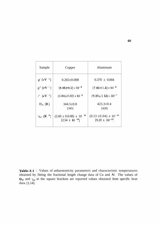
Table-3.1 gives the values of the parameters that give the best fit. The percentage

r.m.s. deviation is found out to be less than 0.3% for both the fits. The values of Qp

obtained from the fits of Cu and Al are respectively (344.5 ± 0.8) K and (423.3 ±

0.4) K which compare well with the corresponding reported values 345 K and 428 K.

The values of the coefficient of the electronic contribution to thermal expansion (-)f/)

obtained from our fits are (2.60 ±0.08) x 10"10K 2 and (9.13 ±0.04) x lO^K" 2 for

Cu and Al respectively which also agree with the reported values. The comparison

is shown in Table-3.1. This impressive agreement between our fitted values and the

ones given in the literature imparts a fair amount of confidence in our approach.

In the following section, we shall use our model to analyze the thermal expansion

data of ferromagnetic transition metals where the electron-magnetic and magnon

terms also contribute. Thi? is followed by application of the model to alkali halides.

58

f-9

120 170 220 270 320

T (K)

Fig.3.4 : Fractional length change data of Copper and Aluminum with the fits tothe eqn.(3.2) shown as the solid lines.

60

Sample

<7'(eV ])

g" (eV"1)

/' (eV"1)

eD(K)

lei (K-2)

Copper

0.265±0.008

(8.86±0.2)xHT6

(1.04±0.02) xUT6

344.5±0.8[345]

(2.60 ± 0.0.08) x 10 10

[2.54 x 10'10]

Aluminum

0.370 ± 0.004

(7.85±1.3)xlO~6

(9.20±1.53)xl0-7

423.3±0.4[428]

(9.13 ±0.04) x 10" 1C)

[9.20 x 10'10]

Table-3.1 : Values of anharmonicity parameters and characteristic temperaturesobtained by fitting the fractional length change data of Cu and Al. The values of©# and 7fJ in the square brackets are reported values obtained from specific heatdata [1,14].

61

3.4 Measurement and Analysis of Thermal Expansion of Nickel and

Iron

Interest in the transition metal elements has continued unabated for several decades

for their interesting magnetic and thermal properties several of which have remained

hitherto elusive. Experimentally, ferromagnetic transition metals are found to show

in addition to a vibrational contribution a linear-T dependence in their low tem-

perature thermal expansion behaviour which is believed to include both the pure

electronic contribution and a contribution from the itinerant electron moments. As

we have already mentioned in subsection 3.2.3, this linear-T term in the thermal

expansion coefficient is commonly referred to as the electron-magnetic contribution

and can be explained within the framework of the collective electron model of Stoner

and Wohlfarth. There have been a host of experimental reports giving the values of

electron-magnetic Griineisen parameter Fg". But accurate theoretical calculation of

Fg" is certainly very difficult for these elements because of their complicated band

structure and complex magnetic behaviour. To our knowledge, there has been only

one calculation of Fg" [22] wliich predicted F£" = 5/3 from a simplified model for

magnetic properties of electrons in isolated d-bands based on the works of Lang and

Ehrenreich [23] and Heine [24]. However there seems to be no justification for this

model to apply in general.

We have also discussed in the subsection-3.2.4 that in the transition metals and

alloys the magnetic contribution to the thermal expansion may come from the lo-

calized spin moments too which we have termed as magnon contribution. To our

knowledge, for these materials there exists no estimation of the magnon Griineisen

62

parameter (F™9). which is essentially given by the volume derivative of the Heiscn-

berg interaction energy J, again a quantity difficult to calculate theoretically.

The aim of the present section is to show that our model can be used together

with the band structure results to analyze the thermal expansion data of transition

metals to yield reliable estimates of characteristic temperatures, various contribu-

tions to specific heat and the Griineisen parameters. For this purpose we have per-

formed thermal expansion measurements on two transition metals, namely nickel

and iron for which accurate band structure calculations are available. We have

already discussed in detail in Chapter 2 our thermal expansion measurement pro-

cedure and have also presented our fractional length change data of Fe and Ni in

2.5 for the sake of comparison with the reported data. In the following subsections

(3.4.1 and 3.4.2), we shall present the analysis of these data using our model.

3.4.1 Nickel

Band structure calculations for Ni [25,26] show that the 3d-band electron wave

functions overlap strongly with 4s-band electrons. It has been found that at zero

temperature the outermost electrons are distributed so that the Ni d-band contains

9.4 electrons per atom and s-band contains 0.6 electrons per atom. The upspin

d-subband is completely filled up with 5 electrons per atom while the downspin

d-subband has 4.4 electrons per atom. Thus the d-band contains 0.6 holes' per atom

which are the participating particles in the ferromagnetism of Ni. Therefore

which explains why Ni is considered a strong itinerant ferromagnet [27]. Further-

more, the occupied part of the up-spin d-subband has a width of 4.6 eV and that

(3.88)

63

of the down-spin d-subband has a width of 4.08 eV with an exchange splitting of

0.52 eV.

To analyze the thermal expansion behaviour of Ni we have fitted the fractional

length data to eqn.(3.2) with the total average lattice displacement (x)r given by

eqn.(3.7) and (x)p', (x)™g and (x)pT

h obtained from eqns.(3.74), (3.85) and (3.14)

respectively. Fits have been performed with Co = 1 and with g' = g/c2a(T0), g"

= g2/(?, /' = / / c 2 , ©£>, 0£, p, A, m and 7' as parameters. It is observed that

p = 3 gives the best fit. This shows the absence of optical modes in the present

system. Furthermore, the magnon contribution also turns out to be negligibly small.

In the final fit, therefore, the Einstein and the magnon terms have been dropped

altogether. The fit is shown in Fig.3.5. It is clear that the fit is excellent over the

entire range of temperature. The percentage r.m.s. deviation is found to be about

0.7%. Table-3.2 gives the parameter values for the best fit. Interestingly enough,

the value of the Debye temperature obtained from our fit is 450 K which is exactly-

identical to the value reported in the literature [14]. Using the fitted values of the

anharmonic parameters and the Debye temperature and with the total number of

atoms, .V — 6.023 x 102"1, we now obtain the molar vibrational specific heat (CPH)

from eqn.(3.18). T$ is then calculated from eqn.(3.20) using BT - 1.86 x 1011

NnT2 [14]. V = 6.59 cc (molar volume) and the above value of M. It is observed

that TVQ remains essentially constant, independent of temperature in the range 80 -

300K and we find its value to be equal to 2.0 which compares quite favourably with

the value 1.6 (see Table-3.3) which is the reported lattice Griineisen parameter for

Ni at low temperature [1].

The value of m obtained from fitting is 0.497 which suggests that in the case of

Ni the energy band is almost parabolic. Using the fitted values of m, A and Q> =

64

Fig.3.5 : Fractional length change data of Iron and Nickel with the fits to theeqn.(3.2) shown as the solid lines.

Using this value of cM and NM = 0.6, BT = 1.8G x 1011 Nm~2, V = 6.59 cc

(molar volume) and the fitted values of A and m we obtain from eqn.(3.76), 6

= 1.97 which is in excellent agreement with the reported experimental electron-

magnetic Griineisen parameter value 2.1 (see Table-3.3) [1]. The coefficient of the

molar electron-magnetic specific heat can now be easily calculated from eqn.(3.73).

We get 7fm = 7.243 mJ/mol K2 which agrees remarkably well with the reported

experimental value, 7.02 mJ/mol K2 [14] lending credence to our theoretical analysis.

3.4.2 Iron

Band structure calculations on iron by Callaway and collaborators [28,29] suggest

that at zero temperature the upspin d-subband of iron contains 4.6 electrons per

atom within a band width of 4.7 eV and the downspin d-subband contains 2.4

electrons within a width of 3.4 eV with an exchange splitting of 1.3 eV. We thus

65

1 we find *)-'rm = 3.1 x 10"9 K 2 which is in excellent agreement with the reported

value, 3.8 x 10~9 K~2 [1]. To obtain the electron-magnetic specific heat and F£"

we need to know the value of the hole band width, eOd- In the absence of exchange

interactions each d-subband of Ni contains 4.7 electrons at OK within a band width

of 4.34 eV. If w' is the total band width of the d-band (i.e., the width including the

occupied electron band and the hole band) at T = OK in the absence of exchange

interactions, then we can write

(3.89)

which yields w' — 4.523 eV and thus e^ is obtained as

eod - (4.523 - 4M0)eV = 0.183eV . (3.90)

66

Sample

9' (eV-])

9" (eV"1)

/ ' (eV-1)

eD (K)

7?)

A (K-2)

->;m ( K - 2 )

y « , ( K - 5 / 2 )

Nickel

0.21±0.02

(3.24±0.2)xl0~3

(3.83±0.2)xl0-"

450.0±0.7[450]

0.497±0.002

(1.23 ±0.7) x 10 9

3.1 x 10*9

[3.8 x 10~9]

-

Iron

0.16 ± 0.02

(2.63±0.2)xl0-3

(3.092±0.2)xl0"'1

469.7±0.7[470]

0.489±0.002

(1.95 ±0.6) x 10 9

4.9 x 10 9

[3.2 x lO"9]

(2.9 ±0.6) x 10 10

Table-3.2 : The fitted parameter values for Ni and Fe. The values of Debyetemperatures inside the square brackets are taken from ref.14 and the values of f'tinside square brackets are taken from ref.l.

67

have Nod: = 0.4 and A^i = 2.6 and therefore the relative magnetisation for iron at

T = OK is given by

which implies that iron is not a strong itinerant ferromagnet [27]. The fractional

length change data for iron are fitted to eqn.(3.2) with the above value of Co and with

9', 9" 1 ft ©D> ©£i Pi A, in and -)mnj as fitting parameters. It is again observed that

p = 3 gives the best fit. So the final fit has been carried out without the Einstein

term. It is however interesting to note that it was not possible to fit the data with

reasonable accuracy without the magnon term which is however consistent with the

observation that Co < 1 for iron. The fit is shown in Fig.3.4. Clearly the fit is

excellent. The percentage r.m.s. deviation is found to be about 0.3%. Table-3.2

gives the parameter values from the best fit. The value of 0/; obtained from the

fit is 469.7 K which is again in excellent agreement with tin' value quoted in the

literature (see Table-3.2) [14].

We calculate F^1 for Fe in the same way as we have discussed for Ni. We find

for Fe, F '̂1 = 1.485 which agrees quite remarkably with the reported value 1.3 [1].

From the fitted values of m and A and with Co = 0.73, we obtain 7 ,̂, = (4.956 ±

0.6) x 10~9 K 2. which compares reasonably with the reported value (3.2 ± 0.4) x

1Q-9 j^-2 jjj j u t n e a r j s e n c c of exchange interactions each d-subband of Fe contains

3.5 electrons at OK within a band-width of 4.05 eV. Using the same prescription as

was followed in the case of Ni, we find for Fe, w = 5.146 eV and thus e0<i = 1.096

eV. Using this value of eod, and Nod = 3.0, BT = 1.683 x 10n Nm"2 [14], 7VO = 6.023

x 1023, V = 7.09 cc (molar volume) and the fitted values of A and m, we obtain

fromeqn.(3.77), 6 = 2.01 which is fairly close to the reported experimental value 2.4

68

Sample

Nickel

Iron

->m, (mJ/molK2)

7.243[7.02]

8.829[4.980]

i t

2.00[1.6]

1.481.3]

IT

1.97[2.1]

2.01[2.4]

G

4.01

Table-3.3 : The estimated values of the electron-magnetic contribution to specificheat and Gruneisen parameters of Ni and Fe. The values of ->em inside the squarebrackets are taken from ref.14 and the values of Gruneisen parameters inside squarebrackets are taken from ref.l.

69

[1]. From eqn.(3.73) we now get -)fm = 8.829 mJ/mol K3 which is somewhat higher

than the only reported value 4.98 mJ/mol K- [1]. As has already been alluded

to above, we have obtained a nonvaaishing magnon contribution to the thermal

expansion of iron with 7 ^ = 2.878 x 10 10 K-5/2. Using the expression (3.87)

and the prescription that the magnon entropy should continuously go over to the

paramagnetic value Rln2 at T — Tc. r) is then found to be equal to 4.01. Eqn.(3.84)

then yields, -y,^ = 0.257 mJ/mol K~5^2 which is about an order of magnitude larger

than the only reported value [32]. So it seems that more accurate measurements

together with careful analysis of data are called for to verify the magnon contribution

to the specific heat and thermal expansion of Iron.

Thus we find that our method provides us with very accurate values of the

Debye temperature, yields estimates of the anharmonicity parameters of the lattice

potential, gives correct values the Griineisen parameters and suggests the nature of

the energy bands. We show that both nickel and iron have almost parabolic bands.

We furthermore show that the electron-magnetic moments in nickel are all itinerant

while those in iron are not. We would like to point out that in addition to the

assumption of volume independence of £Oi we have made a few more assumptions

in our analysis for the sake of mathematical simplicity. For instance, we have used

the low-temperature limit of the Stoner model. This, we believe, will introduce

only a small error in our result because for both nickel and iron the temperature

range considered in our work is much below the transition temperature. Secondly,

we have neglected a small electronic contribution which would come from the s-

band. We have also neglected the band transfer effect, which is proportional to

{kBT/tod}2 and is therefore very small in the present case for both iron and nickel.

Finally, the expression for the maguou contribution used in our analysis is rigorously

70

valid only at long wavelengths and at low temperatures at which the system can

have only low-lying excitations. In practice however this turns out to be a good

enough approximation in many cases. Incorporation of the contributions from the

s-band and the band transfer effect and the higher-order electron-magnetic and

magnon terms will certainly improve our analysis. We however do not anticipate

any significant qualitative difference to show up, although a marginal change in the

model parameters might be expected.

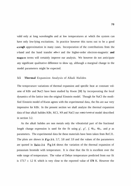
3.5 Thermal Expansion Analysis of Alkali Halides

The temperature variations of thermal expansion and specific heat at constant vol-

ume of KBr and NaCl have been studied by Kwon [30] by incorporating the local

dynamics of the lattice into the original Einstein model. Though for NaCl the modi-

fied Einstein model of Kwon agrees with the experimental data, the fits are not very

impressive for KBr. In the present section we shall analyze the thermal expansion

data of four alkali halides KBr, KC1, KI and NaCl our semiclassical model described

in section 3.2.

As the alkali halides are non metals only the vibratioiial part of the fractional

length change expression is used for the fit using g', g", f, ©#, ©£, and p as

parameters. The experimental data for these materials have been taken from Ref.31.

The plots are shown in Figs.3.6, 3.7, 3.8 and 3.9 and the values of the parameters

are quoted in Table-3.4. Fig.3.6 shows the variation of the thermal expansion of

potassium bromide with temperature. It is clear that the fit is excellent over the

wide range of temperature. The value of Debye temperature predicted from our fit

is 173.7 ± 1.2 K which is very close to the reported value of 174 K. However the

71

Fig.3.6 : Temperature variation of fractional length change data of KBr with thesolid line showing the fit to the data.

72

Fig.3.7 : Temperature variation of fractional length change data of NaCl with thesolid line showing the fit to the data.

73

Fig.3.8 : Temperature variation of fractional length change data of KCl with thesolid line showing the fit to the data.

74

Fig.3.9 : Temperature variation of fractional length change data of KI with the solidline showing the fit to the data.

fit did not show the presence of any optical modes. In Fig.3.7 the data of NaCl

is plotted with the fit which is given by the solid line. The fit is quite impressive

over the complete temperature range The average number of phonon branches p

in this case, however, comes out to be a fraction,i.e., 3.2 which is probably because

the parameter p is kept fixed over the entire range of temperature while in reality

the number of phonon branches excited in different temperature ranges could be

different. Interestingly, however, the value of Debye temperature obtained from our

fit is 321.0 ± 1.3K which is identical to the value reported in literature. The value

of Einstein temperature returned by the fit is 649.8 ± 1.3 K. Fig.3.8 shows the

variation of thermal expansion of potassium chloride with temperature. Evidently

the fit is fairly good over the entire temperature range and the value of Debye

temperature obtained from our analysis is 236.6 ± 0.8 K which is again quite close

to the reported value 235 K. The average number of phonon branches in this case

came out to be 5 with the Einstein temperature as 540.2 ± 0.8 K. Finally in Fig.3.9

the behaviour of the thermal expansion data of potassium iodide is plotted as a

function of temperature. The fit is quite impressive at the complete temperature

range. The value of Debye temperature predicted from the fit is exactly identical to

the value quoted in literature which is 132.0 K. But the total number of branches

came our to be 3. Thus in general the above semiclassical theory seems to agree

quite well with the experimental results. One can see the distinct advantage of this

model is that it predicts the values the Debye and Einstein temperatures from the

thermal expansion data quite accurately. Hence the same model can be used to

calculate the vibrational specific heat and the vibrational entropy using the fitted

parameters from the fit of the thermal expansion data.

75

76

3.6 Conclusion

In this chapter we have developed a new microscopic theoretical model to obtain

the vibrational, electron-magnetic and magnon contributions to the coefficient of

thermal expansion. The model has been applied to analyze the thermal expan-

sion behaviour of simple elemental metallic systems like Cu and Al. ferromagnetic

transition metals such as Fe and Ni and alkali halides. It has been shown that the

present model provides us with estimates of anharmonicity parameters of the lattice

potential and also gives very accurate values of the characteristic Debye and Ein-

stein temperatures. We have furthermore shown that we are able to obtain from

our approach quite successfully the values of the various Griineisen parameters.

The model developed in the present chapter will be used to analyze the thermal

expansion behaviour of more complicated systems in the subsequent chapters.

77

References

[1] T.H.K. Barrou, J.G. Collins and G.K. White, Adv. Phys. 29. 609 (1980).

[2] G. Leibfried and W. Ludwig, Solid State Phys. 12, 276 (1961).

[3] H.R. Glyde and M.L. Klein, Crit. Rev. Solid St. Sci. 2, 18 (1971).

[4] G.K. Horton and A.A. Maradudin, Dynamical Properties of Solids, Vols.l and

2 (Amsterdam, North Holland. 1974, 1975).

[5] M.L. Klein and J.A. Venables (editors). Rare Gas Solids, Vol.1 (Academic-

Press. London. 1976).

[6] G.D. Mukherjee, C. Bansal and Ashok Chatterjee, Mod. Phys. Lett. B 8,

425 (1994).

[7] G.D. Mukherjee, Ashok Chatterjee and C Bansal, Physica C 232, 241 (1994)

[8] G.D. Mukherjee, C. Bansal and Ashok Chatterjee, Phys. Rev. Lett. 76, 1876

(1996).

[9] G.D. Mukherjee, C. Bansal and Ashok Chatterjee, Vibrational and mag-

netic contribution to entropy of an Ll> ordered and a pariially ordered

NisMn alloy : results from thermal expansion measurements and model

calculations, submitted for publication.

[10] E.C. Stoner, Proc. Roy. Soc. A165, 372 (1938); A169, 339 (1939).

[11] E.P. Wohlfarth, Proc. Roy. Soc.(London) A195. 434 (1949); Proc. Phys.

Soc. 60, 360 (1948).

78

[12] E.P. Wohlfarth, Phil. Mag. 42, 374 (1951).

[13] O. Madelung, Introduction to Solid State Physics (Springer, Berlin. Heidel-

berg, 1978), p.314.

[14] C. Kittel, Introduction to Solid State Physics (Wiley Eastern Univ. Edition,

1977).

[15] J.G. Collins and G.K. White, Prog. Low temp. Phys. 4, 40 (1964).

[16] D.C. Wallace, J. Appl. Phys. 41, 5055 (1970).

[17] A.H. Morrish, The Physical Principles of Magnetism, (Robert E. Kreiger Pub-

lishing Co., Inc., 1980).

[18] F. Bloch, Z. Physik 57. 545 (1929); L. Brillouin, J. Phys. Radium 3, 565

(1932).

[19] J.C. Slater, Phys. Rev. 49, 537 (1936); 49, 931 (1936); 52, 198 (1937); Revs.

Mod. Phys. 25, 199 (1953)

[20] F.R. Kroeger and C.A. Swenson. J. Appl. Phys. 48. 853 (1977).

[21] P.R. Bevington, Data Reduction and Error Analysis for the Physical Sciences,

(Me Graw Hill, New York, 1969), p.204.

[22] M. Shimuzu, Phys. Lett. A 50, 93 (1974).

[23] N.D. Lang and H. Ehrenreich, Phys. Rev. 168, 605 (1968).

[24] V. Heine, Phys. Rev. 153, 673 (1967).

[25] J. Callaway and C.S. Wang, Phys. Rev. B 7, 1096 (1973).

7Q

[26] C.S. Wang and J. Callaway. Phys. Rev. B 9, 4892 (1974).

[27] E.P. Wohlfarth, Ferromagnetic Materials, vol.1 (ed. E.P. Wohlfarth. North-

Holland, Amsterdam, 1980), p.l.

[28] R.A. Tawil and J. Callaway, Phys. Rev. B 7, 4242 (1973).

[29] J. Callaway and C.S. Wang. Phys. Rev. B 16, 2095 (1977).

[30] T.H. Kwon, Phil. Mag. Lett. 65. 261 (1992); Solid State Commun. 82. 1001

(1992).

[31] R.K. Kirby, T.A. Hahn and B.D. Rothrock, Thermal Expansion, American

Institute of Physics Handbook, 3rd Edition, ed. D.E. Gray. 4-119 (1972).

[32] M. Dixon, F. Hoare, T.M. Holden and D.E. Moody, Proc. Roy. Soc. A285,

561 (1965).