chapter 3 uncertainty in spatial trajectories

Chapter 3

Uncertainty in Spatial Trajectories

Goce Trajcevski

Abstract This chapter presents a systematic overview of the various issues and so-lutions related to the notion of uncertainty in the settings of moving objects tra-jectories. The sources of uncertainty in this context are plentiful: from the merefact that the positioning devices are inherently imprecise, to the pragmatic aspectthat, although the objects are moving continuously, location-based servers can onlybe updated in discrete times. Hence come the problems related to modelling andrepresenting the uncertainty in Moving Objects Databases (MOD) and, as a con-sequence, problems of efficient algorithms for processing various spatio-temporalqueries of interest. Given the ever-presence of uncertainty since the dawn of philos-ophy through modern day nano-level science, after a brief introduction, we presenta historic overview of the role of uncertainty in parts of the evolution of the humanthought in general, and Computer Science (CS) and databases in particular, whichare relevant to this chapter. The focus of this chapter, however, will be on the impactthat capturing the uncertainty in the syntax of the popular spatio-temporal querieshas on their semantics and processing algorithms. We also consider the impact ofdifferent models in different settings – e.g., free motion; road-network constrainedmotion – and discuss the main issues related to exploiting such semantic dimen-sion(s) for efficient query processing.

3.1 Introduction

Historically, the impact of the imperfect knowledge on the reasoning and belief hasbeen a topic that has attracted a lot of research interest among both philosophersand logicians [41, 63, 44, 123]. With the advent of the computing technologies,as various domains of Computer Science (CS) have emerged, the importance of

Goce TrajcevskiDept. of EECS, Northwestern University, 2145 Sheridan Rd. Evanston, Il 60208 USA (researchsupported by NSF-CNS-0910952), e-mail: [email protected]

63

mailto:[email protected]

64 Goce Trajcevski

capturing the uncertain/probabilistic nature of the data has been recognized in manyof them:

• Artificial Intelligence which, in a sense popularized the Possible-Worlds seman-tics [6, 40, 158].

• Knowledge Representation and Reasoning along with Logic Programming andDeductive Databases [1, 7, 98, 173].

• Incorporating it on top of the traditional database technology [16].to list but a few.Due to the novel application domains along with advancements in database tech-

nology, a lot of recent research has been undertaken, addressing problems in mod-elling and efficient querying of imprecise/uncertain data [2, 20, 111, 125, 133, 134].In the past two decades, the advances in sensing and communication/networking

technologies, along with the miniaturizations of computing devices and develop-ment of variety of embedded systems have spurred the recognition of the importanceof Location Based Services (LBS) [126] in a plethora of applications. Frommilitary,through structural and environmental monitoring, disaster/rescue management andremediation, to tourist information-providing systems – the efficient management oflarge amount of (location, time) data pertaining to mobile entities over (large) pe-riods of time is a paramount. After several works and development of some ad-hocsolutions [89], the field of Moving Objects Databases (MOD) [56, 163] emergedin the late 1990’s as an enabling technology for the LBS-related applications, pro-viding formal foundations and bringing about development of prototype system-s [51, 69].Contrary to the typical assumptions in:

1. Spatial databases [19, 76, 130, 142], where the data items may have dimension-ality and extent, but are (relatively) static over time;

2. Temporal databases [35, 72, 132], where the main objective is capturing thetime-varying nature of the data in various application domains; and

3. Time-series [79, 78, 116, 177], where the values of the data samples over timeoften pertain to a single dimension,

in MOD-settings, the objects are assumed to move, either freely in the 2D (or even3D) space [90, 52, 131], or constrained by a road network [38, 50, 28, 154]. Themain features of spatio-temporal data sets:

1. The discrete data samples are expected to represent a continuous motion overthe given space, thereby necessitating some type of an interpolation; and

2. The typical queries of interest (e.g., whereabouts-in-time, range, (k)nearest-neighbor, reverse nearest-neighbor, skyline) are continuous – which is, theiranswers need to be re-evaluated in time, or even persistent (cf. [131]) – whichis, in addition to re-evaluating the answers over time, one may need to take intoconsideration the entire history of the motion;

have influenced a large body of works addressing issues related to modelling/ repre-sentation, indexing and querying such data [9, 14, 24, 80, 37, 99, 109, 59, 112, 71,93, 60, 97, 105, 164, 102, 119, 106, 140, 139, 141, 155, 169, 172]

3 Uncertainty in Spatial Trajectories 65

In practice, the location data at different time-instants is obtained by some po-sitioning devices like, for example, a GPS-enabled device on-board a moving ob-jects, which eventually transmits the location to a MOD server(s). However, GPSreceivers only approximate the actual position of the respective sensor or object dueto physical limitations and measurement errors of the sensing hardware [27].The position data may be obtained by some other (collaborating) tracking-

devices e.g., roadside sensors [26]. Even more so in application settings like intrusion-detection and environmental monitoring, where the tracking of the moving object ofinterest is based on collaborative trilateration and continuous hand-off among theparticipating sensors [39, 137, 62, 110, 136, 176, 179, 180]. In addition to the inter-polation in-between consecutive location samplings, the imprecision of the devicesinvolved, both GPS-based as well as sensor-based, is yet another source of uncer-tainty. But another example of location imprecision is the investigation of trajecto-ries of various particles in physical and chemical processes [121].Motivated by these observations, many researchers have focused on addressing

the problem of uncertainty management in MOD settings [5, 21, 31, 30, 67, 66, 83,85, 86, 91, 94, 108, 113, 115, 114, 143, 149, 145, 159, 160], also considering theimpact of the restriction of the motions to road networks [5, 31, 30, 45, 84, 83, 178].While it is often the case to assume that the possible locations of a given objectat a particular time-instant is obeying a uniform distribution within certain bounds,recent works have addressed the impact of the different pdfs [21, 67, 159].An important observation when it comes to incorporating uncertainty into the

processing of spatio-temporal queries is that, in order to relieve the user from fac-toring it out from the answers, it needs to be incorporated in the very syntax of thegiven query [18, 88, 103, 115, 149, 145, 148, 171]. Although many of the existingworks have focused on uncertain point-objects with (mostly) linear motion with con-stant speed in-between updates, some recent results have addressed the uncertaintyaspects of points/lines with extent [157], and even uncertain fields [43, 170]. Suchmodels are necessary to capture, for example, the trajectory of the ”eye” of a givenhurricane [152] – however, in addition to the ”eye” being uncertain, the (moving)spatial zone affected by that hurricane is also uncertain.This chapter gives an overview of the research results in the field of managing and

querying uncertain trajectories data, in a manner that will strike a balance betweenthe breadth and the depth of the different topics presented in the existing literature.The intended goal is to present a body of materials in a manner that will be suit-able for both non-specialists to get introduced to the field, and specialists to get acoherent presentation that could help influence the selection of research directions.In the rest of this chapter, in section 3.2.3, we will overview the historic evolu-

tion of the incorporation and treatment of uncertainty in the philosophy and logic1,as well as certain CS-areas related to AI and databases, along with time-geographyand geometry. Subsequently, Section 3.3.2 will address the role and impact of un-certainty in spatial databases and temporal databases, paving a way for the cruxof the material of this chapter which will follow in Sections 3.4 and 3.5. After a

1 It is well beyond the scope of this chapter to discuss the importance and the treatment of uncer-tainty in all the different scientific fields like, for instance, physics, chemistry, etc.

66 Goce Trajcevski

brief formal overview of the notion of trajectories and spatio-temporal queries2,we will focus on a thorough analysis of the issues related to incorporating the un-certainty into the trajectories’ data model, queries-syntax, and the correspondingprocessing algorithms. Specifically, Section 3.4 will present uncertainty models forfree-space motion as well as models of uncertainty for motion restricted to road net-work. Subsequently, in Section 3.5, we consider the issues that uncertainty bringsin the query processing, and we present examples of different (type of query, un-certainty model) couplings. Section 3.6 concludes this chapter and gives a briefoverview of the role of trajectories uncertainty in a broader context and applicationsettings.

3.2 Uncertainty Throughout the History

We now discuss the evolution of the treatment of the uncertainty along differentaspects of the evolution of the human thought. Firstly, we will review the uncertaintyof the knowledge/belief and how philosophers and logicians throughout the historyhave addressed its formalization(s). Subsequently, we follow up with discussingthe role and treatment of the uncertainty in the fields of Artificial Intelligence andDatabases. The last part of the section touches upon the fields of time-geographyand inexact geometries.

3.2.1 Philosophy and Logic

As part of the philosophy focusing on principles of valid reasoning, inference anddemonstration, logic has had its presence in many of the ancient civilizations –Babylon, Egypt, China and India – clearly demonstrated in some inference rulesrelated to geometric and astronomical calculations. However, the philosophical for-m of logic that is likely the most influential one for the Western and Islamic cultures,bringing about a symbolic and purely formal axiomatic treatment – is the one de-veloped in ancient Greece, as first formalized by Aristotle. Even the earliest works,however, observed that some aspects of formalizing the thought required the con-cepts of knowledge and/or belief, leading to the so called epistemic logic [13] whichfocuses on their systematic properties. The syntax of epistemic logic extends thepropositional logic with the unary operator Ka (or Ba) applied to the traditionalpropositions. Thus, BaP denotes ”the agent a Believes P”, where P is any proposi-tion, and its meaning/semantics is: in all possible worlds compatible with what theagent a believes, it is the case that P [64].Although the epistemic logic has found numerous applications in fields like CS

(AI, Databases) and economics, it was the modal logic [17, 42] that provided a

2 Addressed in greater detail in Chapter 2.


perspective for incorporating the uncertainty into a systematic framework, enablinga qualification of the truth/falsity. Intuitively, a modality is any word or phrase thatcan be applied to a given statement S which, in a sense, creates a new statement thatmakes an assertion about the mode of truth of S – when, where or how S is true (orabout the circumstances under which S may be true) [42]. For a given propositionP, the two main operators of the modal logic are:

1. �: denoting necessity – e.g., �P ≡ it is necessary that P.2. �: denoting possibility – e.g., �P ≡ it is possible that P.

Several approaches have been undertaken towards axiomatization of the modallogic, however, it was not until the work of Kripke [81] that the semantics andmodel-theoretic aspects were fully considered. Given that a particular semantics isas good as its entailment relation (within a given model) can ”mimick” the conse-quence relation in terms of syntactic derivability, the main novelty of the, so called,Kripke structures (or frames) is that they provided a foundation for connecting a par-ticular modal logic to a corresponding class of frames, thereby enabling reasoningabout its (in)completeness. As a specific example, instead of evaluating a compositeformula based solely on the true/false value of its primitive constituents, one mayconsider the behavior of the composite formula when the truth values of the con-stituents are changing gradually from false to true according to some ”scenario”(cf. [29]). A thorough treatment of the topic is well beyond the scope of this chapter– however, the main influence of this line of works is that they brought in agnitioone concept that has been widely used since – the possible worlds3

3.2.2 Uncertainty in AI and Databases

Due to its close relationship with logic and, for that matter, extensive use of theLogic Programming paradigm, AI is one of the very first CS fields that have adoptedthe concept of possible worlds. The Possible Worlds Approach (PWA) is a power-ful mechanism for incorporating new information into logical theories, studied byphilosophers interested in belief revision and scientific theory formation [3], as wellas database theorists [1, 36]. The basic premise of PWA is to keep a single modelof the world that is updated when actions are performed. The update procedure in-volves constructing the nearest world to the current one, in which the consequencesof the actions under consideration hold. As explained in [158], the PWA-based re-vision of a theory can be summed up as: To incorporate a set S of formulae into anexisting theory T, take the maximal subset T of T that is consistent with S, and addS to T. This is one of the approaches undertaken for the problem of minimality ofview updates in databases [46].Although it aimed at bringing about computationally efficient procedures for rea-

soning about actions, PWAwas shown to have problems when it comes to, so called,

3 We respectfully note that philosophers and logicians are likely to disagree that semantics basedon Kripke frames are model-equivalent to the one based possible worlds.

68 Goce Trajcevski

frame, ramification, or qualification issues, due to the fact that it did not distinguishbetween the state of the world and the description of the state of the world [158]. Asa remedy, the Possible Models Approach (PMA) was introduced, which observedthe models of a given theory T, rather than its formulae. The goal of PMA is tochange as little as possible the models of T in order to make the new set of formulaeS true. Once the focus has shifted on the models, reasoning about actions becamemore amenable to incomplete information.The archetypical example of uncertainty in traditional relational databases was

the one of an absence of value for a particular attribute, denoted as NULL. This valueis not associated with a particular type and, more importantly, it implies involvemen-t of the three-valued logic, adding the unknown value in the picture and disturbingthe ”cushy” Closed World Assumption (CWA) model of relational databases. WithNULL value, one is no longer justified to assume that the values stored within adatabase correspond to a complete version of the world and everything not stored inthe database is false – thereby imposing the Open World Assumption and demand-ing extra caution when using SQL in practice.A plethora of novel application domains such as Location-Based services, health

and environmental monitoring based on sensor data analysis, biological image anal-ysis, market analysis and economics – generate a vast amount of data which is in-herently uncertain due to the imprecision of measuring devices, randomness anddelays in data updates. This has spurred a tremendous research interest in proba-bilistic databases [2, 11, 10, 20, 92, 125, 133, 167]. In these settings, one typicalfeature is that some attributes are probabilistic, in the sense that their values are giv-en by a probabilistic density function (pdf) – however, in practice, one cannot hopeto have the pdf available and must rely on samples instead. In general, a probabilisticdatabase can be thought of as finite set of probabilistic tables – one for each plau-sible value of the uncertain tuples, associated with membership probability. If theprobability of a particular instantiation for the objects in the database is greater ze-ro, then that particular instantiation constitutes one of the possible world. The mainproblem is that the cardinality of the set of all the possible worlds is exponentialin the number of uncertain objects [6]. In addition to complicating the issue of thesemantics to the answers of the queries, the large number of possible worlds clearlyimposes computational costs in their processing – enumerating the answers in allthe possible worlds is infeasible in practice. Hence, the researchers have resortedto balancing tradeoff between accuracy and computational cost, e.g., retrieving on-ly objects with highest likelyhood to be in the result; reporting only answers theprobability of which exceeds a given threshold; returning approximate answers, etc.A recent approach addressing a generic query optimization for uncertain databases,introducing a threshold operator (τ -operator) to the query plan and demonstratingthat it is generally desirable to push it ”down” as much as possible, is presentedin [118].Getting into a detailed discussion on the topic of probabilistic databases is be-

yond the scope of this Chapter, and for a comprehensive overview the reader is re-ferred to the recent tutorials [134, 111, 120], along with a cohesive recent collectionof works with an extensive list of references available in [58].


3.2.3 Time-Geography and Inexact Geometries

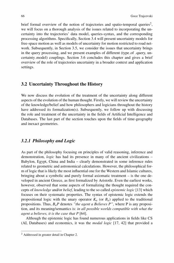
Time geography [61] addresses questions like:Given a location of a mobile agent at time t0, where is the agent at a later time t1 >t0, or where was the agent at a previous time t2 < t0? [160]. Assuming the agent canmove in any direction and is limited only by a maximum speed vmax, time geographyrepresents the reachable locations of this agent by a right cone in (X ,Y,Time)-space.The cone apex represents the agents location at t0, and the aperture represents themaximum speed of the agent – specifically, a cone base Bi represents the set oflocations the agent may settle at a time ti > t0.

Fig. 3.1 Possible Where-abouts of an Agent: differentshades correspond to the pdf’semanating among consecutivetime-instants (cf. [160], withpermission)

Focusing on the discrete probabilistic space-time cone approximation of the con-tinuous pdf of the location of a mobile agent, in [160] three approaches are un-dertaken for deriving that approximation: (1) from a random walk simulation, (2)from combinatorics, and (3) from convolution The results are targeting some basicquestions of interest for time-geography like, for example, what is the most prob-able arrival time of an agent A at a particular location B? We will discuss thespace-time prisms and their implications to trajectories uncertainty in more detail inSection 3.4.While the interest of time geographers is on the uncertainty of location of mobile

agents as the time evolves, a specific type of handling imprecision was consideredby the GIS (Geographic Information Systems) researchers, focusing on the spatialproperties of the basic primitives. Namely, in a vector GIS, the representation isbased on the type of an infinitely small point, in accordance with Euclidean. How-ever, more often than not it is the case that GIS maps are representing geographicentities that have spatial extent. In [123], an axiomatic tolerance geometry was de-veloped, aiming at formalizing the limited capability of distinguishing stimuli invisual perception. Intuitively, the work ”blurred” the concepts of proximity and i-dentity, and developed corresponding primitives for a formalism that can substitutethe traditional concept of ”between”-ness, with an ε-between-ness.

70 Goce Trajcevski

Recently, an attempt of formalizing the geometric reasoning (and computing) foruncertain object was presented in [174], offering an approach based on multiplemodalities of uncertainty in position.The Euclidian geometry is an axiomatic well-founded logical theory, and it has

interpretation of its primitives satisfying its axioms. For example, the Cartesianmodel of Euclidean geometry provides an interpretation of the geometric primitivespoint, line, equality, incidence, congruency, etc..., in the real 2D plane. However,once the uncertainty is allowed for the basic primitives, the logical foundations needto be revisited and novel derivation rules (for developing theorems based on validproofs) are needed. A very recent formalization of the uncertainty into the foun-dation of the Euclidian geometry – the first postulate – and giving interpretationsthat capture the GIS-intuition of points with extension and lines with extension ispresented in [157]. The work extends the Boolean-based reasoning by translatingit into fuzzy logic, providing means of approximating and propagating positionaltolerance within sound inference system.

3.3 Uncertainty in Spatial and Temporal Databases

Two fields that have emerged in the mid/late 1980s – Spatial Databases and Tempo-ral Databases – became, in some sense, precursors to the spatio-temporal databases.In the rest of this section, we present some issues addressed in each field, which areof relevance to the context of this Chapter.

3.3.1 Spatial Databases

Spatial databases [49, 122, 130] deal with efficient storage and retrieval of object-s in space that have identity and well-defined extents, locations, as well as certaingeometric and/or topological relationships among them, owing to developments inapplication fields (GIS, VLSI design, CAD) that needed to deal with large quantitiesof geometric, geographic, or spatial entities. In addition to some stable and matureprototypes prototypes based on solid algebraic type-foundation [48, 55] commer-cial Database Management System (DBMS) vendors have provided extensions totheir products, supporting spatial types and operations (Oracle Spatial, DB2 SpatialExtender, PostgresGIS, Microsoft SQL server, MySQL). Without a doubt, the re-sults in spatial databases have spurred several important research avenues in MODsettings, e.g.:

• Many popular types of MOD queries (e.g., range, nearest-neighbor) have variantsthat were studied in spatial databases context [65, 124].

• Indexing structures developed for facilitating the efficient data access for pro-cessing spatial queries [8, 57] served as foundations for spatio-temporal indexes.


• Topological properties of and relationships among spatial types [32], as wellas generalization issues [156], have also found their ”counter-parts” in spatio-temporal data.

What is of a most specific interest for this Chapter, is that the various conceptsof uncertainty that were investigated in the context of spatial databases have been,in one way or another, applied and/or adopted in the context of uncertain spatio-temporal data.

Fig. 3.2 Processing of SpatialRange Query for UncertainObjects: a.) crisp range; b.)uncertain range (cf. [142],with permission)

The first such concept is the one of location uncertainty. Namely, if one cannotspecifically determine the values of the coordinates of a given point in a referencecoordinate system, then the specification of that point must incorporate the accom-panying uncertainty. We already touched upon the issue of tolerance geometry inSection 3.2.3, which generalized the concept of a point into a point with extensionand investigated the impacts on the formal reasoning in such geometries. In prac-tice, however, in addition to capturing the uncertainty – e.g., via pdf, or histogram,alongside with some boundary – an important aspect is how to incorporate it in thequery processing techniques. The first observation is that the answer to the querymust somehow reflect it. An illustrating example is shown in Figure 3.2, pertainingto processing of spatio-temporal range queries for objects with uncertain locations.Part a.) of Figure 3.2 shows the uncertain object o.ur whose possible locations arebounded by a heptagonal region. For as long as the query region r.q is crisp, one candetermine the probability that o.ur is inside the range r.q – e.g., if the pdf of o.ur isuniform, the probability is: |o.ur∩ r.q|/|o.ur|. However, once the query region itselfis uncertain – e.g., its boundaries have some ε bound of possible whereabouts (cf.Figure 3.2.a.)), then the calculations of the probability become more computation-ally expensive. To cater for this, it was observed in [142] that if one is interestedonly in objects whose probability of being inside the range exceeds certain thresh-old, then a pruning could be applied, for which the U-Tree indexing structure wasintroduced.Many entities such as regions of toxic spread, temperature maps, water-to-soil

boundaries and boundaries among different types of soil, cannot be exactly deter-mined. One of the approaches to address the storing and querying of such data wasto introduce the concepts of fuzzy points, fuzzy lines, and fuzzy regions in the Eu-clidian space. Along with that, fuzzy spatial set operations like union, intersection,

72 Goce Trajcevski

and difference, as well as fuzzy topological predicates were introduced to managespatial joins and selections over fuzzy objects [77, 114, 127, 128].

3.3.2 Temporal Databases

Many applications of databases like, for example, accounting, portfolio manage-ment, medical-record and inventory management record information that is time-varying in nature [35, 72]. At the heart of the temporal databases is the distinctionbetween:

• valid time of a fact, which is the time at which a particular data item is collectedand becomes true as far as the world represented by the database is concerned –possibly spanning the past, present, and future. However, the valid time may notbe known, or recording it may not be relevant for the applications supported bythe database or – in the case that the database models possible worlds – it mayvary across different possible worlds.

• transaction time of a fact, which is the time that a given fact is current in thedatabase. Transaction time may be associated with different database entitieslike, e.g., objects and values that are not facts because they cannot be true or falsein isolation. Thus, all database entities have a transaction-time aspect, which hasa duration: from insertion to (logical) deletion of a given entity.

Capturing the time-varying nature using traditional data models and query lan-guages can be a cumbersome activity and, as a consequence, constructs are neededthat will enable capturing the valid and transaction times of the facts, leading totemporal relations. In addition, query languages [23, 132] are needed with syntacticextensions that enable database operations on temporal models.As an example of uncertainty in temporal databases, consider the following sce-

nario (cf. [12]):Transportation companies (e.g., UPS, DHL) have massive databases containing

information about the various packages they are shipping or have previously shippedand, most importantly, how long it takes for packages to get from a given origin to agiven destination. In such cases, based on the existing data about the valid times, itmay be the case that the database has the following information regarding the arrivaltime for packages departing from oi at 10AM and arriving at d j:

{(12 : 30[0.4,0.6]),(12 : 35[0.3,0.5])}indicating that the probability of a package arriving at 12:30PM is between 0.4 and0.6, and the probability of a package arriving at 12:35PM is between 0.3 and 0.5.A similar scenario in the context of trajectories uncertainty occurs, for example,

when the (location,time) data is obtained via tracking. In addition to the location im-precision, due to the clocks-skew among the sensors participating in tracking [135].In such cases, even if a crisp location is detected after trillateration, the value of thetime attribute will be bound to an interval instead of an instant.


3.4 Modelling Uncertain Trajectories

We now focus on the first part of the main topic of this chapter – modelling of un-certainty in spatial trajectories. After a brief overview of some basic spatio-temporalconcepts and definitions, we proceed with detailed discussion of the main aspects ofsome of the existing models for capturing the uncertainty of spatio-temporal data.The last part of this section is dedicated to the uncertainty aspects when the motionof the objects is constrained to a road network.As mentioned in Section 3.1, the (location, time) data capturing the motion of

moving objects is subject to uncertainty for a variety of reasons, at every stageof its generation. The GPS receivers only approximate the actual position [27]hardware. The precision of motion sensors deteriorates with the distance fromtheir own location and, moreover, typically the localization of a tracked object isdone via trillateration, without guaranteeing that every participating node is reli-able [62, 73, 175, 179]. Aside from the location determination per se’ additionalissues arise due to timing synchronization [135], as well as the protocols used fortransmitting the (location,time) information from sensors to MOD or LBS server-s [37, 162]. Last, but not the least – since it is impossible to record the location forevery single time-instant, the interpolation in-between consecutive records yields anuncertainty of the trajectory [74, 88].In a similar spirit to the works that have developed formal models for repre-

senting and querying ”crisp” trajectories – i.e., ones without any uncertainty of themoving objects whereabouts(e.g., [53, 154]), researchers have addressed the prob-lem of generic representation of uncertainty, along with a framework for syntacticcategorization of spatio-temporal queries [88, 103, 171].

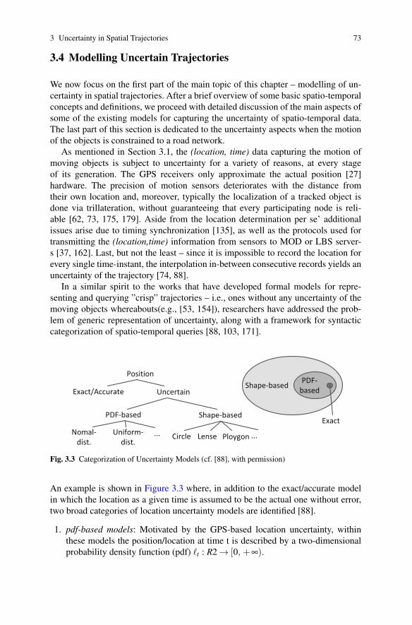
Fig. 3.3 Categorization of Uncertainty Models (cf. [88], with permission)

An example is shown in Figure 3.3 where, in addition to the exact/accurate modelin which the location as a given time is assumed to be the actual one without error,two broad categories of location uncertainty models are identified [88].

1. pdf-based models: Motivated by the GPS-based location uncertainty, withinthese models the position/location at time t is described by a two-dimensionalprobability density function (pdf) �t : R2→ [0, +∞).

74 Goce Trajcevski

2. shape-based models: Bounding the possible locations by geometric shapes (e.g.,circle, lens, polygon), these models may have associated probability values.However, in contrast to the pdf-based models, no claims are made about thespatial pdf within a shape.

Once a model of uncertainty is established, its impact on the syntax of the queriesneeds to be considered, in conjunction with the type of a particular query – e.g.,position, range, nearest neighbor (cf. [88, 103]).In practice, there is a coupling between selecting the model for the motion plan

of the moving objects – affecting the choice of the representation [54, 52] of trajec-tories in a MOD and, consequently, the overall strategy of query processing – andthe uncertainty model. One of the common definitions of a moving object trajectoryis as follows:

Definition 3.1. A trajectory Tr is a function Time→R2, represented as a sequenceof 3D (2D spatial plus time) points, accompanied by a unique ID of the movingobject:

Tri = (oidi, (xi1 ,yi1 , ti1), . . . , (xik ,yik , tik)),

where ti1 < ti2 < .. . < tik .

We note that Definition 3.1 can be used to represent both past trajectories (i.e.,ones whose motion is completed relative to the now-time) as well as future tra-jectories. In future-trajectories settings, users transmit to the MOD server: (1) thebeginning location; (2) the ending location; (3) the beginning time; and (4) possiblya set of points to be visited. Based on the information available from electronic mapsand traffic patterns, the MOD server will construct and transmit the shortest traveltime or shortest path trajectory to the user. This model is applicable to the routingof commercial fleet vehicles (e.g., FedEx and UPS) as well as to web services fordriving directions, where tens of millions of computations of shortest path trajecto-ries are executed monthly by services such as MapQuest, Yahoo! Maps, and GoogleMaps [70].Following are the two noteworthy observations regarding Definition 3.1:

O1: What is (the description of) the location of a given object at a time instantin-between two consecutive points (ti j ≤ t ≤ ti j+1 )?A very common assumption is that in-between two consecutive points, the ob-

jects move along straight line segments and with constant speed, calculated as:

vik =

√(xik − xi(k−1) )

2+(yik − yi(k−1) )2

tik − ti(k−1)(3.1)

Thus, the coordinates of an object oidi at time t ∈ (ti(k−1) , tik) can be obtained bylinear interpolation:

xi(t) = xi(k−1) + vik · (t− ti(k−1) )yi(t) = yi(k−1) + vik · (t− ti(k−1) )

(3.2)

However, researchers have observed that the linear interpolation assumption neednot be suitable for certain applications, especially if prediction of future locations is


needed. Hence, techniques have been proposed for using different (hybrid) modelsbased on representing the objects whereabouts with other algebraic functions [74,138].O2: Are the points arriving at a MOD server in a batch manner, i.e., portions of, orthe entire trip – as opposed to streams of individual (location,time) data values [100,102, 39, 162]?Catering to observations O1 and O2, researchers have proposed several models

of uncertainty of motion, which we address in detail next.

3.4.1 Cones, Beads and Necklaces

An idea discussed in the works of Hagerstrand in the early 1970s in time-geography[61], was the first one to have found its way into MOD research. The first consid-eration of the implications of the fact that the object’s motion was constrained bysome maximal speed vmax in-between two updates was presented in [113]. Based onits definition as a geometric set of 2D points, it was demonstrated that the objectswhereabouts are bound by an ellipse, with foci at the respective point-locations ofthe consecutive updates, as illustrated by the spatial (X-Y) projection in Figure 3.4.Subsequently, [66], presented a spatio-temporal version of the model, naming thevolume in-between two update points a bead4, and the entire uncertain trajectory,a necklace. Note that, in a sense, a bead is a ”backward-extension” of the conceptof spatio-temporal cone as discussed in Section 3.2.3. Namely, the assumption isthat for as long as there is no new (location, time) update, the object can be locatedanywhere inside the cone emanating from the last-known update. However, oncea new update arrives, in addition to the possible-future locations, it also constraintsthe possible locations from the past (since the previous update). A thorough analysisof the properties of the beads was recently done in [85, 86, 108].

Definition 3.2. Let vimax denote the maximum speed that an object can take within

the time-interval (ti, ti+1). A bead Bi = ((xi,yi, ti),(xi+1,yi+1, ti+1),vimax) is defined

as the set of all the points (x,y, t) satisfying the following constraints:

ti ≤ t ≤ ti+1(x− xi)

2+(y− yi)2 ≤ [(t− ti)vi

max]2

(x− xi+1)2+(y− yi+1)

2 ≤ [(ti+1− t)vimax]

2 (3.3)

The first and the second constraint of Equation 3.3, when taken together describe acone emanating upwards from (xi,yi, ti), with a vertical axis and with circles whoseradius value at time t is (t− ti)vi

max, whereas the first and the third constraint togeth-er, specify a cone emanating downwards from (xi+1,yi+1, ti+1), with a vertical axisand with circles whose radius at time t is (ti+1− t)vi

max. Hence, the bead Bi can be

4 We note that, more recently, this model is also called space-time prism.

76 Goce Trajcevski

Fig. 3.4 Spatio-temporalBeads and their (X,Y) Projec-tion

tsv1

t1

t2

tsv2

Possible locations at t = ti

(tsv1 < ti < tsv2)

L1((x1,y1), t1)

L2 ((x2,y2), t2)

ti

viewed as volume defined by the intersection of those two cones. We note that att = ti (resp. t = ti+1) the locations of the object are crisp (i.e., no uncertainty).For a given bead Bi, let di =

√(xi+1− xi)2+(yi+1− yi)2 denote the distance

between locations of the starting location (at ti) and ending location (at ti+1). Also,let tsvi = (ti + ti+1)/2− di/2vi

max and tsvi+1 = (ti + ti+1)/2+ di/2vimax. We observe

that each bead had two distinct types of volumes:

1. Single disk volumes: For every t ∈ [ti, tsvi ], the spatial boundary of the bead att is a circle with radius r(t) = vi

max(t − ti), centered at (xi,yi). Similarly, forevery t ∈ [tsvi+1 , ti+1], the spatial boundary of the bead at t is a circle with radiusr(t) = (ti+1− t)vi

max, centered at (xi+1,yi+1). Hence, throughout [ti, tsvi ], the 3Dvolume of the bead consists of a single cone, with a vertex at (xi,yi, ti) (similarlyfor [tsvi+1 , ti+1]).

2. Two-disks volume: In-between tsvi and tsvi+1 , (i.e., t ∈ [tsvi , tsvi+1 ]), the boundaryof the bead at t is an intersection of two circles: Ci

down(t), centered at (xi,yi),with radius rdown(t) = (t− ti)vi

max, and Ciup(t), centered at (xi+1,yi+1), with ra-

dius r(t) = (ti+1− t)vimax.

We conclude this section with noting one more property of the beads: the projec-tion of the bead Bi onto the the (X ,Y ) plane is an ellipse (cf. [86, 113]), with foci at(xi,yi), and (xi+1,yi+1), and with equation:

(2x− xi− xi+1)2

(vimax)

2(ti+1− ti)2+

(2y− yi− yi+1)2

(vimax)

2(ti+1− ti)2− (xi+1− xi)2− (yi+1− yi)2= 1 (3.4)


We will use Eli to denote the ellipse resulting from projecting the bead Bi in the(X ,Y ) plane. Figure 3.4 provides an illustration of the different components of the(volume of the) bead and its corresponding shapes at different time-points, as pro-jected on the horizontal (X ,Y ) plane.

Definition 3.3. Given a trajectory Tr, its corresponding uncertain trajectory UTr isa sequence of beads, B1, B2, . . . , Bn−1.A Possible Motion Curve PMC(Tr) of UTr is any function f: Time → R2 for

which every point (x,y, t), is either a vertex of the polyline of Tr, or it satisfies(x,y) = f (t) and is inside the corresponding bead – i.e., (∀t)(ti < t < ti+1) ⇒((x,y, t) ∈ Bi).

The concept of a possible motion curve is illustrated in Figure 3.4 and we notethat, in a sense, each possible motion curve corresponds to a ”possible world” of theobject’s motion in-between two updates.We note that in a recent work [94], an analogy is used between the expected-

trajectory (i.e., the line segment between consecutive points) where necklace is re-served for the ”known” part of the motion, and the uncertain part termed ”pendant”.

3.4.2 Sheared Cylinders

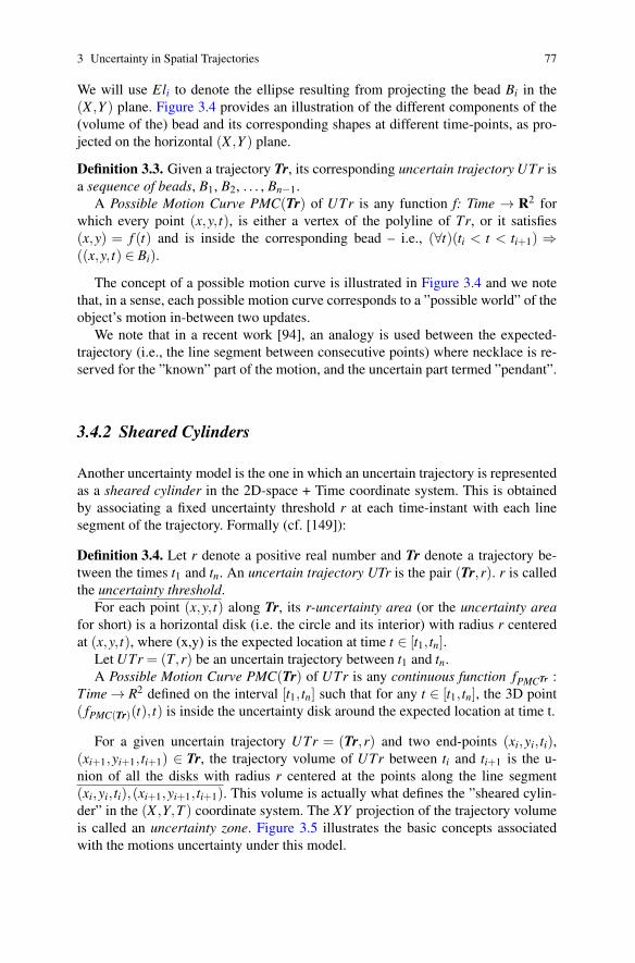
Another uncertainty model is the one in which an uncertain trajectory is representedas a sheared cylinder in the 2D-space + Time coordinate system. This is obtainedby associating a fixed uncertainty threshold r at each time-instant with each linesegment of the trajectory. Formally (cf. [149]):

Definition 3.4. Let r denote a positive real number and Tr denote a trajectory be-tween the times t1 and tn. An uncertain trajectory UTr is the pair (Tr,r). r is calledthe uncertainty threshold.For each point (x,y, t) along Tr, its r-uncertainty area (or the uncertainty area

for short) is a horizontal disk (i.e. the circle and its interior) with radius r centeredat (x,y, t), where (x,y) is the expected location at time t ∈ [t1, tn].LetUTr = (T,r) be an uncertain trajectory between t1 and tn.A Possible Motion Curve PMC(Tr) of UTr is any continuous function fPMCTr :

Time→ R2 defined on the interval [t1, tn] such that for any t ∈ [t1, tn], the 3D point( fPMC(Tr)(t), t) is inside the uncertainty disk around the expected location at time t.

For a given uncertain trajectory UTr = (Tr,r) and two end-points (xi,yi, ti),(xi+1,yi+1, ti+1) ∈ Tr, the trajectory volume of UTr between ti and ti+1 is the u-nion of all the disks with radius r centered at the points along the line segment(xi,yi, ti),(xi+1,yi+1, ti+1). This volume is actually what defines the ”sheared cylin-der” in the (X ,Y,T ) coordinate system. The XY projection of the trajectory volumeis called an uncertainty zone. Figure 3.5 illustrates the basic concepts associatedwith the motions uncertainty under this model.

78 Goce Trajcevski

Fig. 3.5 Uncertain Trajectorybounded by Sheared Cylin-ders, and Possible MotionCurves

X

Y

Time

possible route

possible motion curve

trajectory volumebetween t1 and t3

uncertainty zone

(x1,y1,t1)

(x2,y2,t2)

(x3,y3,t3)

3.4.3 Uncertainty on Road Networks

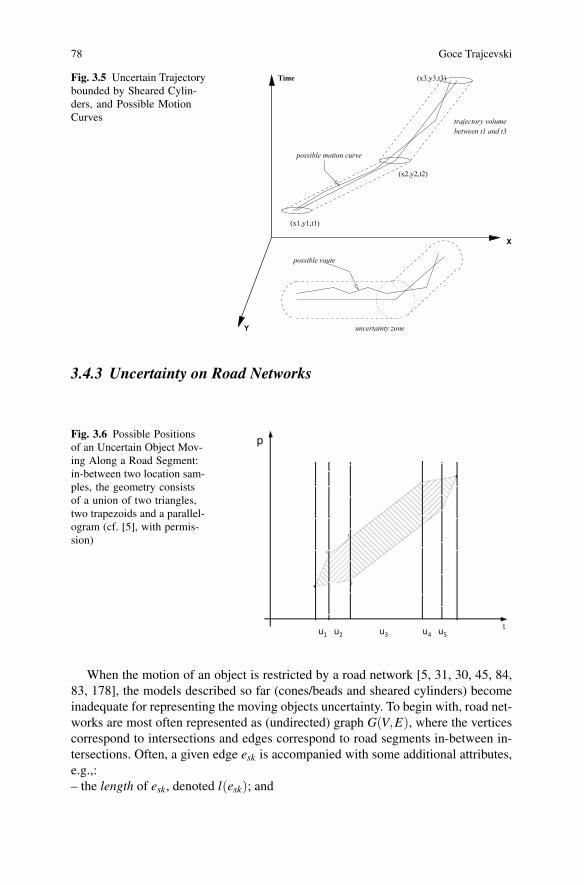
Fig. 3.6 Possible Positionsof an Uncertain Object Mov-ing Along a Road Segment:in-between two location sam-ples, the geometry consistsof a union of two triangles,two trapezoids and a parallel-ogram (cf. [5], with permis-sion)

When the motion of an object is restricted by a road network [5, 31, 30, 45, 84,83, 178], the models described so far (cones/beads and sheared cylinders) becomeinadequate for representing the moving objects uncertainty. To begin with, road net-works are most often represented as (undirected) graph G(V,E), where the verticescorrespond to intersections and edges correspond to road segments in-between in-tersections. Often, a given edge esk is accompanied with some additional attributes,e.g.,:– the length of esk, denoted l(esk); and


– the maximum speed of esk, denoted vmaxsk , which is the upper bound on how fast an

object can move along edge esk.Rich algebraic specification (types, operators) for representing and querying

moving objects on road networks has been presented in [50]. In [5], the authorshave extended the corresponding framework by adding data types to represent stat-ic (unqpoint) and mobile (munqpoint) point objects with location uncertainty,along with a detailed specification of the the respective set of predicates/operators.As shown in Figure 3.6, assuming that the location samples at given time-instantsare ”crisp”, the geometric shape bounding the possible whereabouts of the object isa union of three ”zones”.

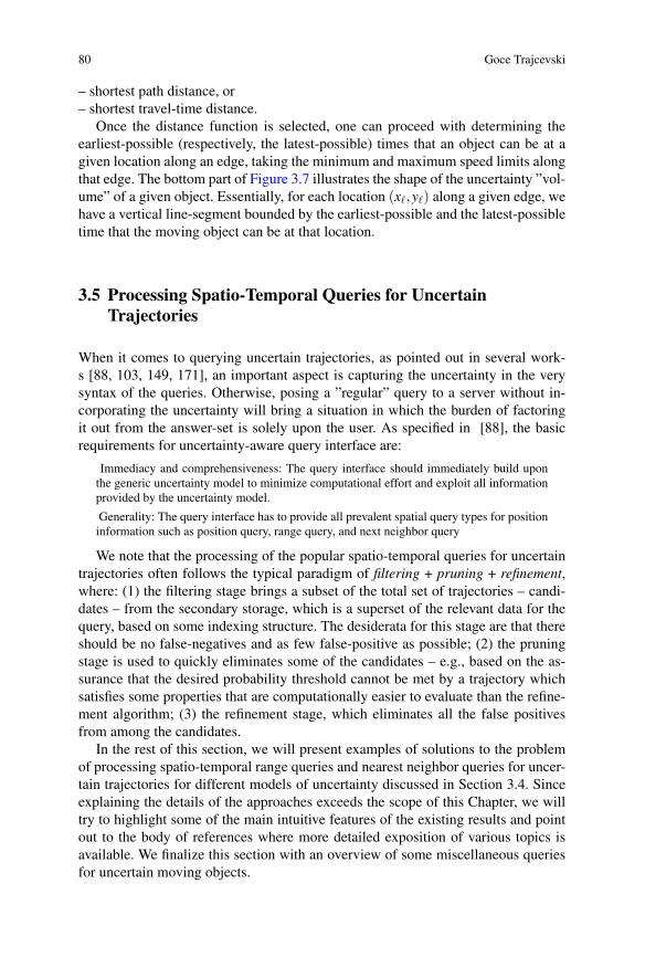
Fig. 3.7 Uncertainty onRoad Networks: The pos-sible whereabouts of themoving objects, contrary tothe space-time prisms, is nowonly a subset of the 2D ellipse– the one intersecting theedges. The cones/beads arereduced to unions of verticalline-segments, ”sweeping”along, and perpendicular toroad network edges (cf. [84],with permission)

The connection (and restrictions) with the beads model is illustrated in Fig-ure 3.7. Note that in road network settings, one cannot consider the entire ellipse (the2D projection of the bead [113]) as a spatial range of the objects possible locations.Instead, only a subset of it intersecting the edges of the graph can be taken intoaccount [84, 83].An important consequence of the model of road network trajectories is that the

distance between two moving objects can no longer be measured using the 2D Eu-clidian distance (L2-norm) since the objects are constrained to move along the edgesof the road network. Instead we need to rely on the shortest network distancewhich,in turn, may have a two-fold interpretation ( [67, 105, 129, 168]):

80 Goce Trajcevski

– shortest path distance, or– shortest travel-time distance.Once the distance function is selected, one can proceed with determining the

earliest-possible (respectively, the latest-possible) times that an object can be at agiven location along an edge, taking the minimum and maximum speed limits alongthat edge. The bottom part of Figure 3.7 illustrates the shape of the uncertainty ”vol-ume” of a given object. Essentially, for each location (x�,y�) along a given edge, wehave a vertical line-segment bounded by the earliest-possible and the latest-possibletime that the moving object can be at that location.

3.5 Processing Spatio-Temporal Queries for Uncertain

Trajectories

When it comes to querying uncertain trajectories, as pointed out in several work-s [88, 103, 149, 171], an important aspect is capturing the uncertainty in the verysyntax of the queries. Otherwise, posing a ”regular” query to a server without in-corporating the uncertainty will bring a situation in which the burden of factoringit out from the answer-set is solely upon the user. As specified in [88], the basicrequirements for uncertainty-aware query interface are:

Immediacy and comprehensiveness: The query interface should immediately build uponthe generic uncertainty model to minimize computational effort and exploit all informationprovided by the uncertainty model.

Generality: The query interface has to provide all prevalent spatial query types for positioninformation such as position query, range query, and next neighbor query

We note that the processing of the popular spatio-temporal queries for uncertaintrajectories often follows the typical paradigm of filtering + pruning + refinement,where: (1) the filtering stage brings a subset of the total set of trajectories – candi-dates – from the secondary storage, which is a superset of the relevant data for thequery, based on some indexing structure. The desiderata for this stage are that thereshould be no false-negatives and as few false-positive as possible; (2) the pruningstage is used to quickly eliminates some of the candidates – e.g., based on the as-surance that the desired probability threshold cannot be met by a trajectory whichsatisfies some properties that are computationally easier to evaluate than the refine-ment algorithm; (3) the refinement stage, which eliminates all the false positivesfrom among the candidates.In the rest of this section, we will present examples of solutions to the problem

of processing spatio-temporal range queries and nearest neighbor queries for uncer-tain trajectories for different models of uncertainty discussed in Section 3.4. Sinceexplaining the details of the approaches exceeds the scope of this Chapter, we willtry to highlight some of the main intuitive features of the existing results and pointout to the body of references where more detailed exposition of various topics isavailable. We finalize this section with an overview of some miscellaneous queriesfor uncertain moving objects.


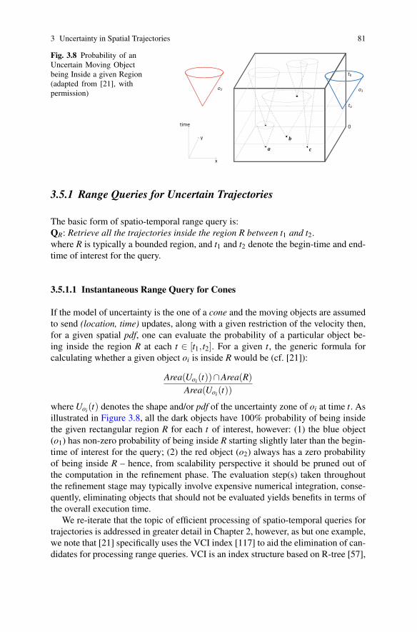
Fig. 3.8 Probability of anUncertain Moving Objectbeing Inside a given Region(adapted from [21], withpermission)

3.5.1 Range Queries for Uncertain Trajectories

The basic form of spatio-temporal range query is:QR: Retrieve all the trajectories inside the region R between t1 and t2.where R is typically a bounded region, and t1 and t2 denote the begin-time and end-time of interest for the query.

3.5.1.1 Instantaneous Range Query for Cones

If the model of uncertainty is the one of a cone and the moving objects are assumedto send (location, time) updates, along with a given restriction of the velocity then,for a given spatial pdf, one can evaluate the probability of a particular object be-ing inside the region R at each t ∈ [t1, t2]. For a given t, the generic formula forcalculating whether a given object oi is inside R would be (cf. [21]):

Area(Uoi(t))∩Area(R)Area(Uoi(t))

whereUoi(t) denotes the shape and/or pdf of the uncertainty zone of oi at time t. Asillustrated in Figure 3.8, all the dark objects have 100% probability of being insidethe given rectangular region R for each t of interest, however: (1) the blue object(o1) has non-zero probability of being inside R starting slightly later than the begin-time of interest for the query; (2) the red object (o2) always has a zero probabilityof being inside R – hence, from scalability perspective it should be pruned out ofthe computation in the refinement phase. The evaluation step(s) taken throughoutthe refinement stage may typically involve expensive numerical integration, conse-quently, eliminating objects that should not be evaluated yields benefits in terms ofthe overall execution time.We re-iterate that the topic of efficient processing of spatio-temporal queries for

trajectories is addressed in greater detail in Chapter 2, however, as but one example,we note that [21] specifically uses the VCI index [117] to aid the elimination of can-didates for processing range queries. VCI is an index structure based on R-tree [57],

82 Goce Trajcevski

with an extra data in its nodes, which is vmax - the maximum possible speed of theobjects under a given node, with an extra storage of the overall maximum speedat leaf nodes. The construction of VCI is similar to the R-tree, with an additionalprovision of ensuring that vmax is correctly maintained at the root of each sub-tree –which is properly considered when a node split occurs. When VCI is used to processa given query, one must account for the changes of the position (with respect to thestored value) over time. To cater for this, in [21] the Minimum Bounding Rectan-gles (MBR) used to process a give query at a time instant t are expanded by a factorof vmax× (t− t0), where t0 is the time of recording the entry for a given object atVCI. We note that the discussion above illustrates techniques that can be applied forprocessing range queries over uncertain trajectories at a particular time-instant.

3.5.1.2 Continuous Range Queries for Sheared Cylinders

In Section 3.4, we introduced the concept of a possible motion curve for a giventrajectory (PMC(Tr)) and hinted that, in some sense, it describes a ”possible world”of a particular trip taking place. However, the generic form of a range query QRdiscussed above does not reflect this anywhere in its syntax. Towards that, the worksin [150, 149] have identified the different qualitative relationships that an uncertaintrajectory (i.e., the family of its PMC’s) could have with the spatial aspect (regionR) and temporal aspect (time-interval of interest [t1, t2]) of the range query.Firstly, since the location of the object changes continuously, the condition of

the moving object being inside R may be true sometime (∃t) or always (∀t) within[t1, t2]. Secondly, an uncertain moving object, in addition completely failing to beinside R, may either possibly or definitely satisfy the spatial aspect of the conditionat a particular time-instant t ∈ [t1, t2]. In simpler terms, if some PMC(Tr) is inside Rat t, there is a possibility that it has been the actual motion of the object – however,this need not be the case as there may have been another PMC(Tr) that the objecthas taken along its motion. Let V Tr denote the bounding volume of (the unionof) all the possible motion curves for a given trajectory Tr – i.e., the sequence ofsheared cylinders (cf. Figure 3.5). Formally, the concept of possibly can be specifiedas ∃PMC(Tr)⊂V Tr and the one of definitely can be specified as ∀PMC(Tr)⊂V Tr.Given the two domains of quantification – spatial and temporal – with two quan-

tifiers each, we have a total of 22 ·2!= 8 operators, and their combinations yield thefollowing variants of the spatio-temporal range query for uncertain trajectories:

• QPSR : Possibly Sometime Inside(T ,R,t1,t2) (∃PMC(TR))(∃t)Inside(R,PMC(TR), t)Semantics: true iff there exists a possible motion curve PMC(Tr) and there existsa time t ∈ [t1, t2] such that PMC(Tr) at the time t, is inside the region R.

• QPAR : Possibly Always Inside(Tr,R,t1,t2)

(∃PMC(Tr))(∀t)Inside(R,PMC(Tr), t)Semantics: true iff there exists a possible motion curve PMC(Tr) of the trajectoryT which is inside the region R for every t in [t1, t2].Intuitively, this predicate captures the fact that the object may take (at least one)specific possible route, which is entirely contained within the region R, during


Fig. 3.9 Illustration of the Predicates Capturing the Different Quantifiers of Spatial and TemporalDomains

the whole query time interval.

• QAPR : Always Possibly Inside(Tr,R,t1,t2)

(∀t)(∃PMC(Tr))Inside(R,PMC(Tr), t)Semantics: true iff for every time value t ∈ [t1, t2], there exists some (not neces-sarily unique) PMC(Tr) inside (or on the boundary of) the region R at t.

• QADR : Always Definitely Inside(Tr,R,tb,te)

(∀t)(∀PMC(Tr))Inside(R,PMC(Tr), t)Semantics: true iff at every time t ∈ [t1, t2], every possible motion curve PMC(Tr)of the trajectory Tr, is in the region R. Thus, no matter which possible motioncurve the object takes, it is guaranteed to be within the query region R throughoutthe entire interval [t1, t2].

• QDSR : Definitely Sometime Inside(Tr,R,tb,te)

(∀PMC(Tr))(∃t)Inside(R,PMC(Tr), t)Semantics: true iff for every possible motion curve PMC(Tr) of the trajectoryTr, there exists some time t ∈ [t1, t2] in which the particular motion curve isinside the region R. Intuitively, no matter which possible motion curve withinthe uncertainty zone is taken by the moving object, it will intersect the regionat some time t between tb and te. However, the time of the intersection may bedifferent for different possible motion curves.

• QSDR : Sometime Definitely Inside(Tr,R,tb,te)

(∃t)(∀PMC(Tr))Inside(R,PMC(Tr), t)Semantics: true iff there exists a time point t ∈ [t1, t2] at which every possibleroute PMC(Tr) of the trajectory Tr is inside the region R. In other words, nomatter which possible motion curve is taken by the moving object, at the specifictime t the object will be inside the query region.

Figure 3.9 illustrates the intuition behind plausible scenarios for the predicates spec-ifying the properties of an uncertain trajectory with respect to a range query, project-

84 Goce Trajcevski

ed in the spatial dimension. Dashed lines indicate the possible motion curve(s) dueto which a particular predicate is true, whereas the solid lines indicate the expectedroutes, along with the boundaries of the uncertainty zone.A couple of remarks are in order:

1. Although we mentioned that there are 8 combinations of the quantifiers overthe variables in the predicates, we listed only 6 of them. This is actually a s-traightforward consequence of the facts from First Order Logic – namely, forany predicate P, given a constant A and variables x and y, it is true that:

(∃x)(∃y)P(A,x,y)≡ (∃y)(∃x)P(A,x,y)

and(∀x)(∀y)P(A,x,y)≡ (∀y)(∀x)P(A,x,y)

This is regardless of the domain of (interpretation of) the variables and the se-mantics of the predicate P. Hence, we have that Possibly Sometime Inside isequivalent to Sometime Possible Inside; and Definitely Always Inside is equiv-alent to Always Definitely Inside. Hence, in effect we have 6 different predi-cates.

2. Similarly, the formula:

(∃x)(∀y)P(A,x,y)⇒ (∀y)(∃x)P(A,x,y)

is a tautology. In effect, this means that the predicate Possibly Always Insideis stronger than Always Possibly Inside, in the sense that whenever Possi-bly Always Inside is true, Always Possibly Inside is guaranteed to be true.We observe that the converse need not be true. As illustrated in Figure 3.9, thepredicate Always Possibly Inside may be satisfied due to two or more possiblemotion curves, none of which satisfies Possibly Always Inside by itself. Whenthe region R is convex, however, those two predicates are equivalent (cf. [149]).

3. For the same reason as above, we conclude that Sometime Definitely Inside isstronger than Definitely Sometime Inside, however, the above two predicatesare not equivalent when the region R is convex. In Figure 3.9 this is shownby R2 satisfying Definitely Sometime Inside, however, since it does not con-tain the entire uncertainty disk at any time-instant, it cannot satisfy Some-time Definitely Inside.

The algorithms for processing the respective predicates involve techniques fromComputational Geometry (CG) (Red-Blue Intersection; Minkowski Sum/Difference)and their detailed presentation is beyond the level of detail for this Chapter. Theirdetailed implementation, along with complexity analysis, is available in [149]. Wenote that in the global context of query processing, [149] focused on the refinementstage.In a sense, the predicates described above correspond to the, so called, ”MAY”

and ”MUST” cases for range queries over uncertain trajectories (cf. [104, 103, 162])


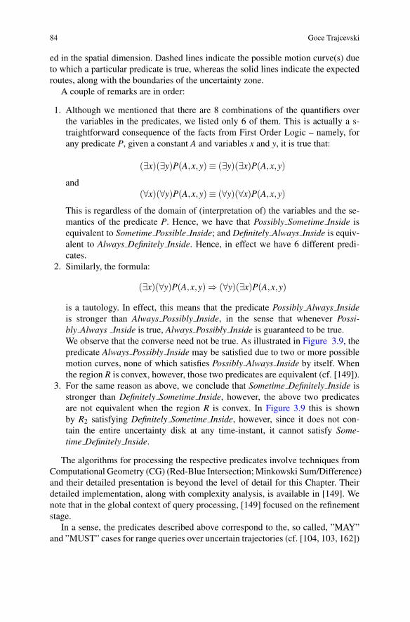
Fig. 3.10 Satisfying the Pos-sibly Sometimes and Pos-sibly Always Predicates forBeads

R

tbq

teq

X

Y

TQuery Prism

Possibly_SometimePossibly_Always(Always_Possibly)

and, more specifically, the ”Inside” property is discussed as a predicate in the genericquery interface discussed in [88].

3.5.1.3 Continuous Range Queries for Beads/Necklaces

As demonstrated in [145], capturing qualitative relationships between a range queryand uncertain trajectories whose uncertainty model is the one of space-time prisms(equivalently, beads) can be done using the same logical formalizations from [149].Not only the same predicates are applicable, but also the relationships among themin terms of Possibly Always Inside being stronger than Always Possibly Inside,and Sometime Definitely Inside being stronger than Definitely Sometime Inside arevalid.The main difference is that the bead as a spatio-temporal structure yields a bit

more complicated refinement algorithms than the ones used in [149] for shearedcylinders. As an illustrating example, Figure 3.10 shows Possible Motion Curvesthat cause the two predicates with existential quantifier over the spatial domain(”Possibly”) to be true.Although the model of beads is more complicated for the refinement stage, it

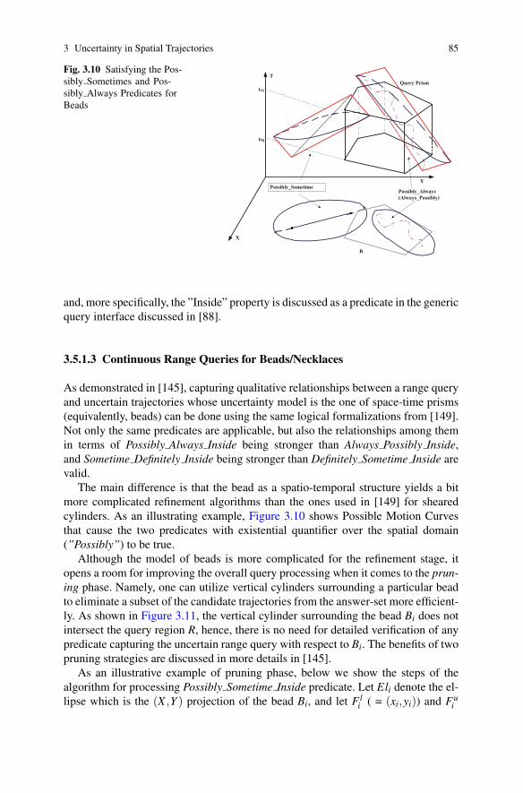
opens a room for improving the overall query processing when it comes to the prun-ing phase. Namely, one can utilize vertical cylinders surrounding a particular beadto eliminate a subset of the candidate trajectories from the answer-set more efficient-ly. As shown in Figure 3.11, the vertical cylinder surrounding the bead Bi does notintersect the query region R, hence, there is no need for detailed verification of anypredicate capturing the uncertain range query with respect to Bi. The benefits of twopruning strategies are discussed in more details in [145].As an illustrative example of pruning phase, below we show the steps of the

algorithm for processing Possibly Sometime Inside predicate. Let Eli denote the el-lipse which is the (X ,Y ) projection of the bead Bi, and let Fl

i ( = (xi,yi)) and Fui

86 Goce Trajcevski

Fig. 3.11 Pruning of Beadswhich do not Qualify for theAnswer of a Range Query

X

Y

T

ai

ai+1

Bi

Bi+1

R

(= (xi+1,yi+1)) denote the 2D projections of its lower and upper foci in temporalsense – i.e., Fl

i occurs at time ti and Fui at time ti+1. For complexity analysis, as-

sume that the region R has m edges/vertices, and an one-time pre-processing cost ofO(m) has been performed to determine the angles in-between its consecutive ver-tices with respect to a given point in R’s interior [107]. The refinement algorithmcan be specified as follows:1. If (ti ∈ [t1, t1]∧Fl

i ∈ R) ∨ (ti+1 ∈ [t1, t2]∧Fui ∈ R)

2. return true

3. else if (Eli∩R �= /0)4. return true

7. return falseEach of the disjuncts in line 1. can be verified in O(logm) due to the convexity of

R (after the one-time pre-processing cost of O(m)) [107]. Similarly, by splitting theellipse in monotone pieces (e.g., with respect to the major axis), one can check itsintersection with R in O(logm), which is the upper bound on the time-complexityof the algorithm.We note that many of the works on formalizing the predicates that capture d-

ifferent types of spatio-temporal range queries are geared towards extending thequerying capabilities of MODs. Consider, for example the following query:QU

R : “Retrieve all the objects which are possibly within a region R, always betweenthe earliest5 time when the object A arrives at locations L1 and the latest time whenit arrives at location L2”.If the corresponding predicates are available, this query can be specified in SQL as:

WITH Earliest(times) ASSELECT When_At(trajectory,L_1)FROM MOD

5 Observe that a given object may pass through a given point along its route more than once


WHERE oid = AWITH Latest(times) AS

SELECT When_At(trajectory,L_2)FROM MODWHERE oid = A

SELECT M1.oidFROM MOD as M1WHEREPossibly_Always_Inside(M1.trajectory,R,

MIN(Earliest.times),MAX(Latest.times))

3.5.1.4 Uncertain Range Queries on Road Networks

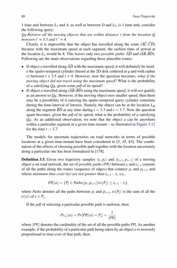
When the motion of a given object is constrained to an existing road network, oneof the sources of its location uncertainty is due to the fact that the objects speed mayvary between some vmin and vmax along a given segment – which we described inSection 3.4.3. However, there is another source of the uncertainty of such motion– namely, the low sampling-rate of the on-board GPS devices e.g., due to unavail-ability of satellite coverage in dense downtown areas. The main consequence of thisis that the distance between two consecutive sampled positions can be large: e.g.,it can be over 1.3km when sampling every 2 minutes, even if a vehicle is movingat the speed as low as 40km/h. The additional uncertainty is reflected in the factthat there may be many possible paths connecting the two consecutively sampledpositions, which satisfy the temporal constraints of the actual consecutive samples.The problem is even more severe for vehicles travelling with higher speeds, as theremay be several intersections between two consecutive samples.

Fig. 3.12 Uncertainty onRoad Networks Due to LowLocation-Sampling Frequen-cy (object may take differentroutes between intersections)

As an example, consider the scenario depicted in Figure 3.12. It shows two con-secutive location-samples: L1 at t1 = 0, and L2 at t2 = 7. There are three possibleroutes between vertices (intersections) A and D: — (AC,CD) with travel time 4 + 2= 6 time units; — AD with travel time of 4; — and (AB,BD), with a travel time of2 + 3 = 5 time units. Given the information about minimum travel time cost – e.g.,

88 Goce Trajcevski

1 time unit between L1 and A, as well as between D and L2, is 1 time unit, considerthe following query:QR:Retrieve all the moving objects that are within distance r from the location Qbetween t’ = 3.5 and t” = 4.Clearly, it is impossible that the object has travelled along the route (AC,CD)

because with the maximum speed at each segment, the earliest time of arrival atthe location L2 would be 8. This leaves only two possible paths: AD and (AB,BD).Following are the main observations regarding these plausible routes:

• If object a travelled along ADwith the maximum speed, it will definitely be insid-e the spatio-temporal cylinder (based at the 2D disk centered at q and with radiusr) between t = 3.5 and t = 4. However, now the question becomes, what if themoving object did not travel using the maximum speed? What is the probabilityof a satisfying QR, given some pdf of its speed?

• If object a travelled along (AB,BD) using the maximum speed, it will not qualifyas an answer to QR. However, if the moving object uses smaller speed, then theremay be a possibility of it entering the spatio-temporal query cylinder sometimeduring the time-interval of interest. Namely, the object can be at the location LQalong the segment BD at any time during t = 3.3 and t = 3.7. Now the questionagain becomes, given the pdf of its speed, what is the probability of a satisfyingQR. As an additional observation, we note that the object a can be anywherewithin a particular segment at a given time-instant – as illustrated in Figure 3.12for the time t = 3.7.

The models for uncertain trajectories on road networks in terms of possiblelocations at a given time-instant have been considered in [5, 45, 83]. The combi-nation of the effects of choosing possible path together with the location uncertaintyalong a particular one has been formalized in [178].

Definition 3.5. Given two trajectory samples (ti, pi) and (ti+1, pi+1) of a movingobject a on road network, the set of possible paths (PPi) between ti and ti+1 consistsof all the paths along the routes (sequence of edges) that connect pi and pi+1, andwhose minimum time costs (tc) are not greater than ti+1− ti, i.e.,

PPi(a) = {Pj ∈ Paths(pi, pi+1)|tc(Pj)≤ ti+1− ti},

where Paths denotes all the paths between pi and pi+1, tc(Pj) is the sum of all thetc(e) of e ∈ Pj.

If the pdf of selecting a particular possible path is uniform, then:

Pri, j(a) = Pr[PPi(a) = Pj] =1|PPi|

where |PPi| denotes the cardinality of the set of all the possible paths PPi. As anotherexample, if the probability of a particular path being taken by an object a is inverselyproportional to time-cost of that path, then:


Pri, j(a) = Pr[PPi(a) = Pj] =1/tc(Pj)

∑Px∈PPi(a) 1/tc(Px)

Even if a particular path Pj is considered, the location of the moving object ata given time-instant t ∈ (ti, ti+1) need not be crisp (i.e., certain) because the speedalong Pj may fluctuate. However, the set of possible locations can be restricted asfollows:

Definition 3.6. Given a path Pj ∈ PPi(a), the Possible Locations of a given movingobject a with respect to Pj at t ∈ [ti, ti+1] is the set of all the positions p along Pjfrom which a can reach pi (respectively, pi+1) within time period t−ti (respectively,ti+1− t) i.e.,

PLi, j(t) ={

p ∈ Pj

∣∣∣∣ tcPj(pi, p)≤ t− titcPj(p, pi+1)≤ ti+1− t

}(3.5)

As an example, in the case of a uniform pdf, the probability that the object a isbetween positions pA and pB along a possible path Pj, whose network-distance isd(pA, pB), is:

Pr[pa(t) ∈ [pA, pB]] = Pri, j(a) · d(pA, pB)

PLi, j(t)(3.6)

where PLi, j(t) denotes the the network-length of PLi, j(t). Formula 3.6 illustratesthe joint consideration of the probability that a particular path Pj is being selectedfrom among the possible ones, together with the probability of the object beingsomewhere along the segment pA, pB at a given time-instant t [178].Clearly, given an existing road-map along with the (location,time) samples, a

methodology is needed to construct all the possible trajectories that satisfy the tem-poral constraints of the samplings. In addition, one needs to determine the pdfs ofthe location uncertainty along different possible paths. Algorithmic solutions fortwo types of probabilistic range queries: snapshot (instantaneous) and continuous,are presented in [178], along with a novel indexing structure – Uncertain TrajectoryHierarchy (UTH), used to index the road network, object movement and trajectoriesin a hierarchical style and to improve the overall efficiency of the query processing.

3.5.2 Nearest-Neighbor Queries for Uncertain Trajectories

We now present some of the techniques that have addressed variants of the problemof efficient management of Nearest-Neighbor (NN) queries for uncertain trajecto-ries. Before we proceed with the details, we note that an assumption commonlyused in the literature (e.g., [21, 142]) is that the locations of the uncertain objectsare independent random variables.The basic form of spatio-temporal range query is:

QNN : Retrieve the nearest neighbors of the trajectory Truq between t1 and t2.

90 Goce Trajcevski

where Truq denotes the uncertain querying trajectory.

3.5.2.1 NN Query for Cone Uncertainty Model

Recall Figure 3.8 used to explain the intuition behind spatio-temporal range queryprocessing for cone-like model of uncertainty. If we take a horizontal ”slice” at aparticular time-instant, we will obtain all the spatial locations of the objects at thattime-instant.

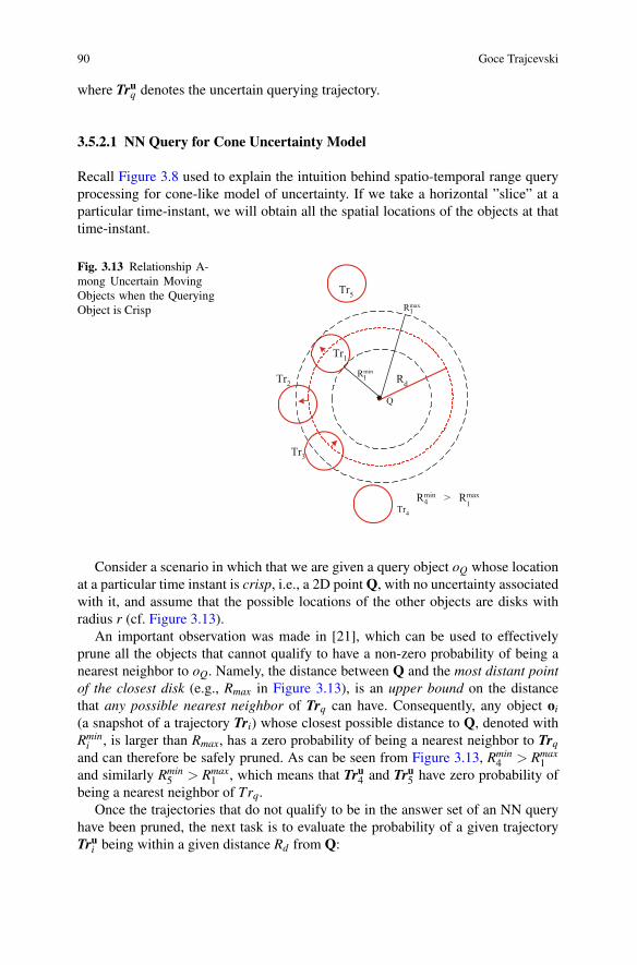
Fig. 3.13 Relationship A-mong Uncertain MovingObjects when the QueryingObject is Crisp

Rmin

Rmax

Q

Tr1

Tr2

Tr3

Tr4

Tr5

Rmin > Rmax

Rd1

1

14

Consider a scenario in which that we are given a query object oQ whose locationat a particular time instant is crisp, i.e., a 2D pointQ, with no uncertainty associatedwith it, and assume that the possible locations of the other objects are disks withradius r (cf. Figure 3.13).An important observation was made in [21], which can be used to effectively

prune all the objects that cannot qualify to have a non-zero probability of being anearest neighbor to oQ. Namely, the distance between Q and the most distant pointof the closest disk (e.g., Rmax in Figure 3.13), is an upper bound on the distancethat any possible nearest neighbor of Trq can have. Consequently, any object oi(a snapshot of a trajectory Tri) whose closest possible distance to Q, denoted withRmin

i , is larger than Rmax, has a zero probability of being a nearest neighbor to Trqand can therefore be safely pruned. As can be seen from Figure 3.13, Rmin

4 > Rmax1

and similarly Rmin5 > Rmax

1 , which means that Tru4 and Tru5 have zero probability ofbeing a nearest neighbor of Trq.Once the trajectories that do not qualify to be in the answer set of an NN query

have been pruned, the next task is to evaluate the probability of a given trajectoryTrui being within a given distance Rd from Q:


PWDi,Q (Rd) =

∫ ∫A

pdf i(x,y)dxdy (3.7)

where A, the integration bound, denotes the area of the intersection of the diskwith radius Rd centered at Q and the uncertainty disk of Tri, with a correspond-ing pd fi(x,y).Then, in order to calculate the probability that the trajectory of a given object,

Truj , is a nearest neighbor of the crisp querying object Trq at a given time instant,one needs to consider:

1. The probability of Tr j being within distance ≤ Rd from Trq; combined with:2. The probability that every other object Tri (i �= j) is at a distance greater than

Rd from the location Q of Trq; and3. The fact that the distributions of the objects are assumed to be independent fromeach other.

Using these observations, the generic formula for the nearest-neighbor probability(cf. [21]) is:

PNNj,Q =

∫ ∞

0pd f WD

j,Q (Rd) ·∏i �= j

(1−PWDi,Q (Rd))dRd (3.8)

As pointed out in [21], the boundaries of the integration need not be 0 and∞ becausethe effective boundary of the region for which an object can qualify to be a nearestneighbor of Trq is the ring centered atQ with radii Rmin and Rmax. More specifically,pd f WD

j,Q (Rd) is 0 for any Rd < Rminj and 1−PWD

i,Q (Rd) is 1 for Rd < Rmini .

By sorting the objects that have a non-zero probability of being nearest neighborsaccording to the minimal distances of their boundaries from Q, one can break theevaluation of the integral from Equation 3.8 into subintervals corresponding to eachRmini and the computation of the PNN

j,Q can be performed in a more efficient manner,based on the sorted distances and the corresponding intervals [21]. The importanceof this observation is in the fact that the the integrals (cf. Equation 3.8) are likelyto be computed numerically. For a uniform pdf of the location uncertainty, the ob-jects can be sorted according to the distances of their expected locations from thequerying object.

3.5.2.2 NN Query for Sheared Cylinders – Continuity and

Time-Parameterization

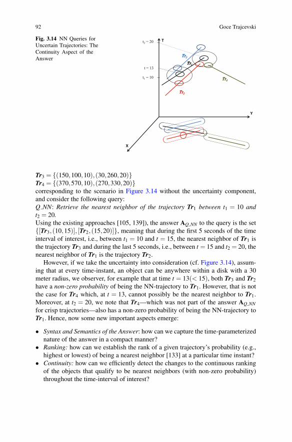
While the methodology explained above is sound for evaluating a snapshot (i.e., in-stantaneous) NN queries, an important property of the NN queries in MOD settingsis that their answer over the time-interval of interest needs to be parameterized [139].In other words, as the querying object itself, as well as the other objects are continu-ously moving, the nearest neighbors will change over time. To illustrate this feature,assume that we have a MOD with four trajectory-segmentsTr1 = {(120,60,10),(220,300,20)}Tr2 = {(310,100,10),(190,260,20)}

92 Goce Trajcevski

Fig. 3.14 NN Queries forUncertain Trajectories: TheContinuity Aspect of theAnswer

Tr3 = {(150,100,10),(30,260,20)}Tr4 = {(370,570,10),(270,330,20)}corresponding to the scenario in Figure 3.14 without the uncertainty component,and consider the following query:Q NN: Retrieve the nearest neighbor of the trajectory Tr1 between t1 = 10 andt2 = 20.Using the existing approaches [105, 139]), the answer AQ NN to the query is the set{[Tr3,(10,15)], [Tr2,(15,20)]}, meaning that during the first 5 seconds of the timeinterval of interest, i.e., between t1 = 10 and t = 15, the nearest neighbor of Tr1 isthe trajectory Tr3 and during the last 5 seconds, i.e., between t = 15 and t2 = 20, thenearest neighbor of Tr1 is the trajectory Tr2.However, if we take the uncertainty into consideration (cf. Figure 3.14), assum-

ing that at every time-instant, an object can be anywhere within a disk with a 30meter radius, we observer, for example that at time t = 13(< 15), both Tr3 and Tr2have a non-zero probability of being the NN-trajectory to Tr1. However, that is notthe case for Tr4 which, at t = 13, cannot possibly be the nearest neighbor to Tr1.Moreover, at t2 = 20, we note that Tr4—which was not part of the answer AQ NNfor crisp trajectories—also has a non-zero probability of being the NN-trajectory toTr1. Hence, now some new important aspects emerge:

• Syntax and Semantics of the Answer: how can we capture the time-parameterizednature of the answer in a compact manner?

• Ranking: how can we establish the rank of a given trajectory’s probability (e.g.,highest or lowest) of being a nearest neighbor [133] at a particular time instant?

• Continuity: how can we efficiently detect the changes to the continuous rankingof the objects that qualify to be nearest neighbors (with non-zero probability)throughout the time-interval of interest?


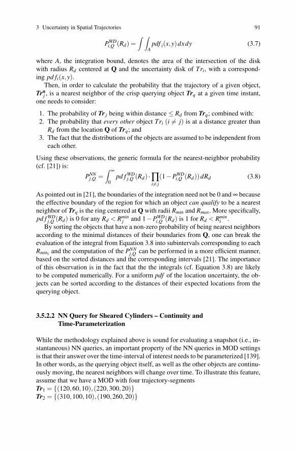
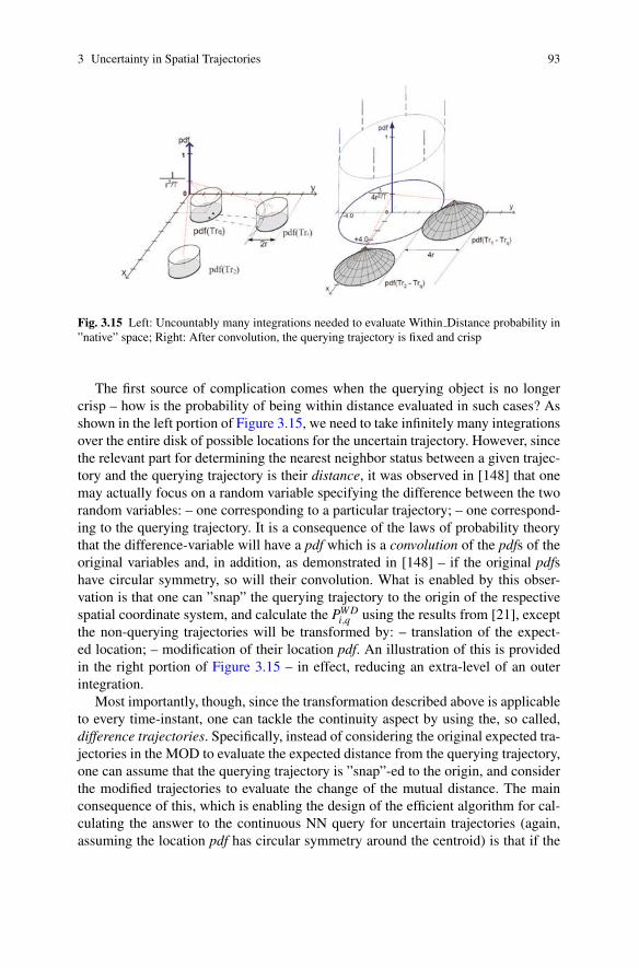
Fig. 3.15 Left: Uncountably many integrations needed to evaluate Within Distance probability in”native” space; Right: After convolution, the querying trajectory is fixed and crisp

The first source of complication comes when the querying object is no longercrisp – how is the probability of being within distance evaluated in such cases? Asshown in the left portion of Figure 3.15, we need to take infinitely many integrationsover the entire disk of possible locations for the uncertain trajectory. However, sincethe relevant part for determining the nearest neighbor status between a given trajec-tory and the querying trajectory is their distance, it was observed in [148] that onemay actually focus on a random variable specifying the difference between the tworandom variables: – one corresponding to a particular trajectory; – one correspond-ing to the querying trajectory. It is a consequence of the laws of probability theorythat the difference-variable will have a pdf which is a convolution of the pdfs of theoriginal variables and, in addition, as demonstrated in [148] – if the original pdfshave circular symmetry, so will their convolution. What is enabled by this obser-vation is that one can ”snap” the querying trajectory to the origin of the respectivespatial coordinate system, and calculate the PWD

i,q using the results from [21], exceptthe non-querying trajectories will be transformed by: – translation of the expect-ed location; – modification of their location pdf. An illustration of this is providedin the right portion of Figure 3.15 – in effect, reducing an extra-level of an outerintegration.Most importantly, though, since the transformation described above is applicable

to every time-instant, one can tackle the continuity aspect by using the, so called,difference trajectories. Specifically, instead of considering the original expected tra-jectories in the MOD to evaluate the expected distance from the querying trajectory,one can assume that the querying trajectory is ”snap”-ed to the origin, and considerthe modified trajectories to evaluate the change of the mutual distance. The mainconsequence of this, which is enabling the design of the efficient algorithm for cal-culating the answer to the continuous NN query for uncertain trajectories (again,assuming the location pdf has circular symmetry around the centroid) is that if the

94 Goce Trajcevski

centroid of Trui −Tru

q is closer to the coordinate-center than the centroid of Truj−Tru

q,then Tru

i has a higher probability of being the nearest neighbor of Truq than Tru

j .Given the observations above, along with the fact that the distance function be-

tween the centroids of the querying trajectory and an individual trajectory changesas a hyperbola [9, 119] over time6 the continuity and ranking aspects can be handledbased on the following properties:

• The nearest neighbor with highest probability will be the trajectory whose dis-tance function determines the lower envelope of the collection of the distancefunction. The rank will change in the cusps of the lower envelope (i.e., wheneverit becomes determined by the distance function of another trajectory).

• The trajectory with the second-highest probability of being a nearest neighborin a given time-interval can be obtained if the one defining the lower envelopein that time-interval is removed (and recursively for the k-th highest probability(k ≥ 2).

• Regardless of the particular pdf, for as long as the uncertainty zone of the object-s’ locations is bounded by a circle with radius r, every trajectory whose distancefunction is further than 4× r from the lower envelope can be pruned from con-sideration for a nearest neighbor with non-zero probability.

Fig. 3.16 Time-parameterization of the An-swer to a Continuous NearestNeighbor Query for UncertainTrajectories (sheared cylindermodel)

When it comes to the structure of the answer that is to be presented to the us-er [148] postulates that one compact structure can be obtained by splitting the time-interval of interest, say [tb, te], into sub-intervals [tb, t1], [t1, t2], . . . , [tn−1, te] so thatthe trajectory that has the highest probability of being the nearest neighbor of Truq ineach sub-interval is unique.Subsequently, each such sub-interval can be further split into its own sub-

intervals – e.g., [ti−1, ti] is split into [ti−1, t(i−1),1], [t(i−1),1, t(i−1),2], . . . , [t(i−1),(k−1), ti].To each of this sub-intervals, again a unique trajectory is matched – representing thetrajectory which would have been the actual highest-probability nearest neighbor ofTruq , if the MOD did not contain Trui−1. Towards that, a tree-structure called IPAC-NN tree (Intervals of Possible Answers to Continuous-NN) was introduced, shownin Figure 3.16 with the following properties:

6 Since squaring each distance function will not disturb the relative ordering, one may readily workwith the corresponding parabolae.


• The root of the tree is node labelled with the description of the parameters ofinterest for the specification of the query, e.g., Truq , along with [tb, te].

• The root has one child for each sub-interval of [tb, te], throughout which thereis a unique uncertain trajectory Trui having the highest probability of being thenearest neighbor to Truq . Each child of the root is labelled with the correspondingtrajectory (e.g., Trui ) and the time-interval of its validity as the highest probabilitynearest neighbor (e.g., ti−1, ti) in Figure 3.16).

• After obtaining the respective labels from the respective parent-node, each child-node checks whether if it is removed from the MOD, there could still be someobject with nonzero probability of being the nearest neighbor of Truq in the timesub-interval of its label.

– If so, then it is an internal node, and each internal node follows the principleof splitting its own (sub)interval like it has been done in the root, and uses thesame labelling for its children.

– If not, then that node is a leaf-node.

The construction of the IPAC-NN tree is based on the algorithm for constructingthe collection of lower envelopes of the distance functions.

3.5.2.3 NN Query for Beads Uncertainty Model

Recall that at the heart of the space-time prisms (beads) is the assumption that themotion of the objects is constrained by some maximal velocity vmax, and the ob-jects can take any speed v ∈ [vmin,vmax] in-between two consecutive (location,time)updates.

Fig. 3.17 Different Cases of Evaluating the Distance Between Two Objects with Uncertain Veloc-ities (cf. [67], with permission)

The assumption for uncertain speed and crisp update points clearly affects howthe minimum possible distance between two objects can vary in-between updates.

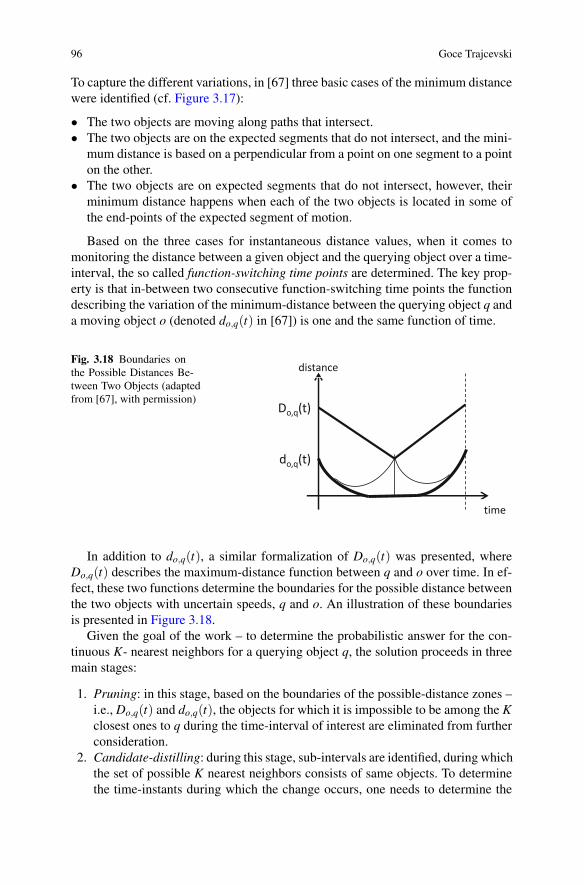
96 Goce Trajcevski

To capture the different variations, in [67] three basic cases of the minimum distancewere identified (cf. Figure 3.17):

• The two objects are moving along paths that intersect.• The two objects are on the expected segments that do not intersect, and the mini-mum distance is based on a perpendicular from a point on one segment to a pointon the other.

• The two objects are on expected segments that do not intersect, however, theirminimum distance happens when each of the two objects is located in some ofthe end-points of the expected segment of motion.

Based on the three cases for instantaneous distance values, when it comes tomonitoring the distance between a given object and the querying object over a time-interval, the so called function-switching time points are determined. The key prop-erty is that in-between two consecutive function-switching time points the functiondescribing the variation of the minimum-distance between the querying object q anda moving object o (denoted do,q(t) in [67]) is one and the same function of time.

Fig. 3.18 Boundaries onthe Possible Distances Be-tween Two Objects (adaptedfrom [67], with permission)

In addition to do,q(t), a similar formalization of Do,q(t) was presented, whereDo,q(t) describes the maximum-distance function between q and o over time. In ef-fect, these two functions determine the boundaries for the possible distance betweenthe two objects with uncertain speeds, q and o. An illustration of these boundariesis presented in Figure 3.18.Given the goal of the work – to determine the probabilistic answer for the con-

tinuous K- nearest neighbors for a querying object q, the solution proceeds in threemain stages:

1. Pruning: in this stage, based on the boundaries of the possible-distance zones –i.e., Do,q(t) and do,q(t), the objects for which it is impossible to be among the Kclosest ones to q during the time-interval of interest are eliminated from furtherconsideration.

2. Candidate-distilling: during this stage, sub-intervals are identified, during whichthe set of possible K nearest neighbors consists of same objects. To determinethe time-instants during which the change occurs, one needs to determine the


time tc when doi,q(tc = Do j ,q(tc) – i.e., the minimum-distance of the object oibecomes equal to the maximum-distance of the object o j with respect to thequerying object q. In this case, if o j was among the PKNN(q) (i.e., possibly a-mong the K nearest neighbors) before tc, then it will be substituted by oi at/aftertc.

3. Ranking: in this phase, a confidence value, based on a reasonable probability-model is determined for each object among the candidates.

In [68], an indexing structure was proposed – TPRe tree – which can be appliedto index trajectories with uncertain velocities, thereby avoiding unnecessary I/O op-erations from the secondary storage. Extending the paradigm from [67], scalableefficient techniques were presented to process probabilistic variants of the K−NNquery, along with a variant of the range query – a moving range (i.e., within a givendistance from a moving object).

3.5.2.4 NN Query for Uncertain Trajectories on Road Networks

As discussed in Section 3.4.3, assuming that the periodic (location,time) samples donot contain any errors, the main source of uncertainty for the objects moving alongroad networks is the fluctuation of the speed between some minimal value vmin andmaximal value vmax. Typically, in these settings, vmax corresponds to some speed-limits dictated for a particular type of road segment (e.g., highway portion vs. streetin downtown area).When it comes to processing NN query on road networks, the key aspect is the

distance function. Contrary to the motion in a free 2D space, where the distance at aparticular time-instant is the L2 – Euclidian distance, as we mentioned in Section 3.4in these settings, the distance can be evaluated only based on the existing network,i.e., the underlying graph representing it [67, 105, 129, 168]. Hence, the typicalstrategies rely on either the shortest path distance, or shortest travel-time distance.A recent approach for tackling Continuous K−NN queries for objects moving

along segments of road networks with Uncertain speeds (CUkNN) has been pre-sented in [91]. In a similar spirit to [67], for a given object o and a querying objectq, two bounding distance-functions are presented:

1. MaxDq,o,(t) determining how the maximum distance between o and q variesover time.

2. MinDq,o,(t) determining how the minimum distance between o and q varies overtime.

When calculating the distance functions, given the bounds vmin and vmax, foreach of o and q at a given time-instant, the closest possible location and the furthestpossible location from a vertex (e.g., an intersection in the graph-based networkmodel) along the direction of movement in the current segment are obtained. Theshortest path distance between the vertices of the graph incident to the edges alongwhich o and q travel, together with the bounds for closest/furthest possible locations,

98 Goce Trajcevski

is used to calculate the total value of MinDq,o,(t) and MaxDq,o,(t). The crux is thatthese two functions – which were hyperbolae for the motion in free 2D space (or,equivalently, parabolae) – now correspond to line segments in the (distance,time)space.The typical CUkNN query processing proceeds with the standard three stages:

pruning – eliminating the objects with zero probability of being one of the K n-earest neighbors of q; refinement – where the possible candidates are ranked; andprobability evaluation – the last phase where the actual probabilities for the object-s from the refinement phase are calculated. We close this part with a note that amethodology for processing NN query in the settings in which a model based onlocation-uncertainty is coupled with a network distance function based on shortesttravel-time has recently been presented in [147]

3.5.3 Potpourri: Some Miscellaneous Queries/Predicates forUncertain Trajectories

The range and nearest neighbor queries have been identified as important categorieseven in traditional databases settings. However, there are certain predicates that aretopological in nature [33, 76] which have recently been considered in the context ofuncertain spatio-temporal data.Given that the beads (or, space-time prisms) can be described by polynomial

constraints (cf. Section 3.4), various queries that are well-suited for constraineddatabase paradigm can be explored. For example, one can envision predicates likeinPrism(r,p,q,v) specifying that the point r is inside the space-time prism defined bypoints p and q, with a maximum speed v, where p is preceding q in time.An example query that is of interest to geographers [61] is the, so called, alibi-

query. Given two space-time prisms, representing the uncertain motions of two in-dividuals, the alibi-query asks whether those objects had a chance to meet – es-sentially, whether their corresponding space-time prisms intersect. It was observedthat relying on the quantifier-elimination approaches for first order theories to pro-cess the alibi-query was computationally cost-prohibitive, and an analytic solutionto this problem was presented in [82].The inside-ness (cf. Section 3.5.1.2) can also be viewed as a topological proper-

ty describing a possible relationship between an uncertain trajectory and a spatio-temporal range corresponding to the query-prism. This is but an example of theperspective taken in [94], where different topological predicates for uncertain tra-jectories under the, so called, pendant model are discussed. The pendant model is,in some sense, equivalent to the beads for moving points, however, the formalizationin [94] addresses both uncertain moving points ( unmpoint) and uncertain movingregions (unmregion). Extending the work in [34] presenting the STP framework forformalizing Spatio-Temporal Predicates, a collection of Spatio-Temporal UncertainPredicates (SUTPs) is presented, based on the pendant model. Formally, a SUTP isa boolean expression containing:


• Topological predicates: disjoint, meet, overlap, covers, coveredBy, equal, inside,contains.

• Traditional logic operators: ¬,∨,∧,∃,∀.• Set expressions: ∪,∩,∈,⊂.• Model-operations: e.g., at instance; temp select (along with the distance function

dist).

An interesting geometric approach towards the scalability aspect of the proba-bilistic NN query processing is presented in [4]. Namely, in a similar spirit to [22],the work introduces the concept of Probabilistic Voronoi Diagram that can be usedto prune the objects that do not qualify to be in the answer set of the NN-query –i.e., ones whose Voronoi cells are not adjacent to the Voronoi cell of the queryingobject.

3.6 Summary

In this Chapter, we presented an overview of the research trends addressing prob-lems related to modelling and querying of uncertain trajectories data. After a select-ed historic overview of the treatment of uncertainty in a few disciplines which, inone way or another, have impacted the evolution of the thought related to the themeof this Chapter, we gave a more focused overview of the uncertainty in the fieldsof spatial and temporal databases. In the last two sections, we gave detailed discus-sions related to different models of trajectories that capture the uncertain data, andthe issues that arise when processing queries over such data.We now bring a few observations regarding the role and impact of trajectories

uncertainty in a broader context and application settings/requirements7:

• In order to reduce the communication and bandwidth consumption, moving ob-jects may have a ”contract” with the MOD server based, e.g., on the distance-based dead-reckoning policy [161, 162]. In these settings, each object will pe-riodically transmit an update of the form (location, time, velocity) and will nottransmit any other location update, for as long as the deviation between the actuallocation (as observed e.g., by the on-board GPS device) and the expected locationin the MOD does not exceed certain threshold. Clearly, in-between updates, theMOD server cannot have any certain knowledge about the objects whereabouts.In the case that the objects are moving along a road-network, clearly, the locationuncertainty can be reduced [45].

• In order to reduce the storage requirements for the large quantities of (loca-tion,time) data, sometimesMOD servers may apply data-reduction techniques [15].Clearly, reducing the size of the data points will ultimately introduce an uncer-tainty, although the size vs. imprecision trade-offs can be managed (e.g., one can

7 Note that Chapter 1 and Chapter 4 address in detail the topics of trajectory data reduction andprivacy, respectively.

100 Goce Trajcevski

guarantee a particular error-bound). Clearly, this will affect the (im)precision inthe answers to the spatio-temporal queries in suchMOD [15]. To couple the man-agement of the transmission cost and storage costs, sometimes one may delegate(part of) the responsibility of spatio-temporal data reduction to the moving ob-jects themselves, asking them to periodically transmit a historic data of their tripafter applying reduction techniques [87, 144]

• In wireless sensor networks scenarios, in the case that some imprecision intime/space is acceptable, some reduction in the (location,time) data-items locallygenerated by the tracking sensors can be spared from transmission to a dedicatedsink. This can significantly contribute towards saving the scarce energy resourcesof the nodes [146, 165], and prolong the network lifetime.

• Another application domain in which the uncertainty arises as a requirement isthe location-privacy [25, 101, 166]. One of the most popular techniques – spatialcloaking – actually blurs the user’s exact location into a cloaked area, satisfyingsome ”quality threshold” – e.g., the available location information contains anuncertainty disk with area larger than the desired threshold.

We believe that the spatio-temporal uncertainty will keep on playing an impor-tant role in many application domains in the future. One challenge is coming upwith a unified model of location and time uncertainties, along with correspondingquery constructs and processing strategies. Many aspects of trajectory data cluster-ing [47, 75] and warehousing [153] will inevitably require a formal treatment ofuncertainty. Similarly, many applications that rely on maintaining spatio-temporalvariograms [96, 151] will need to incorporate some type of uncertainty. One fieldthat could potentially benefit from proper adaptive use of uncertainty is visualizationof mobile data, both in large center displays, as well as limited resolution displayson board moving vehicles [95].

Acknowledgments: Many thanks to Reynold Cheng, Ralf Guting, Yuan-Ko Huang,Bart Kuijpers, Ralph Lange, Markus Schneider, Egemen Tanin, Yufei Tao andStephan Winter (along with their collaborators) for generously permitting the useof some of the figures appearing in their works throughout this Chapter.Special thanks to Hans-Peter Kriegel for his constructive suggestions.

As stated earlier, this Chapter was written with an intention of providing an overviewof the topic of uncertainty in location trajectories in a manner that will balance thebreadth of the coverage vs. depth of exposing the main issues in a few selectedproblems and solutions, as well as a tutorial-like source for both non-experts and re-searchers in the field. Any omissions, with sincere apologies, are sole responsibilityof the author.


References

1. Abiteboul, S., Kanellakis, P.C., Grahne, G.: On the representation and querying of sets ofpossible worlds. In: SIGMOD Conference, pp. 34–48 (1987)

2. Aggarwal, C.C., Yu, P.S.: A survey of uncertain data algorithms and applications. IEEETrans. Knowl. Data Eng. 21(5), 609–623 (2009)

3. Alchourron, C., Gardenfors, P., Makinson, D.: On the logic of theory change. Journal ofSymbolic Logic 50, 510–530 (1985)

4. Ali, M.E., Tanin, E., Zhang, R., Kotagiri, R.: Probabilistic voronoi diagrams for process-ing moving nearest neighbor queries (2011). (personal communication, manuscript underrevision)

5. de Almeida, V.T., Guting, R.H.: Supporting uncertainty in moving objects in networkdatabases. In: GIS, pp. 31–40 (2005)

6. Antova, L., Koch, C., Olteanu, D.: 10(106) worlds and beyond: efficient representation and

processing of incomplete information. VLDB Journal 18(5), 1021–1040 (2009)7. Apt, K., Blair, H.: Arithmetic classification of perfect models of stratified programs. In:R. Kowalski, K. Bowen (eds.) Proc. 5th International Conference and Symposium on LogicProgramming, pp. 765–779. Seattle, Washington (August 15-19, 1988)

8. Beckmann, N., Kriegel, H., Schneider, R., Seeger, B.: The r∗ tree: An efficient and robustaccess method for points and rectangles. In: ACM SIGMOD (1990)

9. Benetis, R., Jensen, C.S., Karciauskas, G., Saltenis, S.: Nearest and reverse nearest neighborqueries for moving objects. VLDB Journal 15(3), 229–249 (2006)

10. Bernecker, T., Emrich, T., Kriegel, H.P., Mamoulis, N., Renz, M., Zufle, A.: A novel proba-bilistic pruning approach to speed up similarity queries in uncertain databases. In: ICDE, pp.339–350 (2011)

11. Bernecker, T., Kriegel, H.P., Mamoulis, N., Renz, M., Zufle, A.: Scalable probabilistic sim-ilarity ranking in uncertain databases. IEEE Trans. Knowl. Data Eng. 22(9), 1234–1246(2010)

12. Biazzo, V., Giugno, R., Lukasiewicz, T., Subrahmanian, V.S.: Temporal probabilistic objectbases. IEEE Trans. Knowl. Data Eng. 15(4), 921–939 (2003)

13. Buh, I.: Epistemic Logic in the Middle Ages. Routledge (1993)14. Cai, Y., Hua, K., Cao, G.: Processing range-monitoring queries on heterogeneous mobileobjects. In: International conference on Mobile Data Management (MDM) (2004)

15. Cao, H., Wolfson, O., Trajcevski, G.: Spatio-temporal data reduction with deterministic errorbounds. VLDB Journal 15(3) (2006)

16. Cavallo, R., Pittarelli, M.: The theory of probabilistic databases. In: VLDB, pp. 71–81 (1987)17. Chellas, B.: Modal Logic: An Introduction. Cambridge University Press (1980)18. Chen, J., Cheng, R., Mokbel, M.F., Chow, C.Y.: Scalable processing of snapshot and contin-uous nearest-neighbor queries over one-dimensional uncertain data. VLDB Journal 18(5),1219–1240 (2009)

19. Chen, T., Schneider, M.: Data structures and intersection algorithms for 3d spatial data types.In: GIS (2009)

20. Cheng, R., Chen, J., Mokbel, M.F., Chow, C.Y.: Probabilistic verifiers: Evaluating con-strained nearest-neighbor queries over uncertain data. In: ICDE (2008)

21. Cheng, R., Kalashnikov, D.V., Prabhakar, S.: Querying imprecise data in moving objectsenvironments. IEEE-Trans. Knowl. Data Eng. 16(9) (2004)

22. Cheng, R., Xie, X., Yiu, M.L., Chen, J., Sun, L.: Uv-diagram: A voronoi diagram for uncer-tain data. In: ICDE, pp. 796–807 (2010)

23. Chomicki, J.: Temporal query languages: A survey. In: ICTL, pp. 506–534 (1994)24. Chon, H.D., Agrawal, D., Abbadi, A.E.: Range and knn query processing for moving objectsin grid model. Mobile Networks and Applications 8 (2003)

25. Chow, C.Y., Mokbel, M.F., Liu, X.: Spatial cloaking for anonymous location-based servicesin mobile peer-to-peer environments. GeoInformatica 15(2), 351–380 (2011)

102 Goce Trajcevski

26. Civilis, A., Jensen, C.S., Pakalnis, S.: Techniques for efficient road-network-based trackingof moving objects. IEEE Trans. Knowl. Data Eng. 17(5) (2005)

27. of Defense, U.S.D.: Navstar gps: Global positioning system standard (2008)28. Demiryurek, U., Pan, B., Kashani, F.B., Shahabi, C.: Towards modeling the traffic data onroad networks. In: GIS-IWCTS (2009)

29. Detlovs, V., Podnieks, K.: Introduction to Mathematical Logic. University of Latvia (2011).Hyper-textbook for students

30. Ding, Z.: Utr-tree: An index structure for the full uncertain trajectories of network-constrained moving objects. In: MDM, pp. 33–40 (2008)

31. Ding, Z., Guting, R.H.: Uncertainty management for network constrained moving objects.In: DEXA, pp. 411–421 (2004)

32. Egenhofer, M., Franzosa, R.: Point set topological relations. International Journal of Geo-graphical Information Systems 5 (1991)

33. Egenhofer, M.J., Dube, M.P.: Topological relations from metric refinements. In: GIS (2009)34. Erwig, M., Schneider, M.: Spatio-temporal predicates. IEEE Trans. Knowl. Data Eng. 14(4),881–901 (2002)

35. Etzion, O., Jajodia, S., (eds.), S.S.: Temporal Databases: Research and Practice. Springer,LNCS (1998)

36. Fagin, R., Ullman, J., Vardi, M.: On the semantics of updates in databases. In: Proc. ACMPODS, pp. 352–365 (1983)

37. Gedik, B., Liu, L.: Mobieyes: A distributed location monitoring service using moving loca-tion queries. IEEE Transactions on Mobile Computing 5(10) (2006)

38. George, B., Kim, S., Shekhar, S.: Spatio-temporal network databases and routing algorithms:A summary of results. In: SSTD (2007)

39. Ghica, O., Trajcevski, G., Zhou, F., Tamassia, R., Scheuermann, P.: Selecting tracking princi-pals with epoch-awareness. In: Proceedings of the 18th ACM SIGSPATIAL GIS Conference,pp. 222–231 (2010)

40. Ginsberg, M.L., Smith, D.E.: Reasoning about action i: A possible worlds approach. Artif.Intell. 35(2), 165–195 (1988)

41. Goguen, J.: The logic of inexact concepts. Synthese 19, 325–373 (1969)42. Goldblatt, R.: Mathematical modal logic: A history of its evolution (2006).Http://homepages.mcs.vuw.ac.nz/ rob/papers/modalhist.pdf

43. Goodchild, M.F., Zhang, J., Kyriakidis, P.C.: Discriminant models of uncertainty in nominalfields. T. GIS 13(1), 7–23 (2009)

44. von Gottfried Wilhelm Leibniz, F.: Theodicy: Essays on the Goodness of God, the Freedomof Man, and the Origin of Evil. Open Court (1998)

45. Gowrisankar, N., Nittel, S.: Reducing uncertainty in location prediction of moving objects inroad networks. In: GIScience (2002)

46. Grant, J., Horty, J., Lobo, J., Minker, J.: View updates in stratified disjunctive deductivedatabases. Journal of Automated Reasoning 11, 249–267 (1993)

47. Gudmundsson, J., van Kreveld, M.J.: Computing longest duration flocks in trajectory data.In: GIS (2006)

48. Guting, R.H.: Gral: An extensible relational database system for geometric applications. In:VLDB (1989)

49. Guting, R.H.: An introduction to spatial database systems. VLDB J. 3(4), 357–399 (1994)50. Guting, R.H., de Almeida, V.T., Ding, Z.: Modeling and querying moving objects in net-works. VLDB Journal 15(2) (2006)

51. Guting, R.H., Behr, T., Duntgen, C.: Secondo: A platform for moving objects database re-search and for publishing and integrating research implementations. IEEE Data Eng. Bull.33(2), 56–63 (2010)

52. Guting, R.H., Bohlen, M.H., Erwig, M., Jensen, C.S., Lorentzos, N., Nardeli, E., Schneider,M., Viqueira, J.R.R.: Spatio-temporal models and languages: An approach based on datatypes. In: Spatio-Temporal Databases – the Chorochronos Approach (2003)

Http://homepages.mcs.vuw.ac.nz/rob/papers/modalhist.pdf


53. Guting, R.H., Bohlen, M.H., Erwig, M., Jensen, C.S., Lorentzos, N., Schneider, M., Vazir-giannis, M.: A foundation for representing and queirying moving objects. ACM TODS(2000)

54. Guting, R.H., Bohlen, M.H., Erwig, M., Jensen, C.S., Lorentzos, N.A., Schneider, M., Vazir-giannis, M.: A foundation for representing and querying moving objects. ACM Trans.Database Syst. 25(1) (2000)

55. Guting, R.H., Schneider, M.: Realm-based spatial data types: The rose algebra. VLDB J.4(2), 243–286 (1995)

56. Guting, R.H., Schneider, M.: Moving Objects Databases. Morgan Kaufmann (2005)57. Guttman, A.: R-trees: A dynamic index structure for spatial searching. In: SIGMOD Con-ference, pp. 47–57 (1984)

58. Haas, P.J., Suciu, D.: Special issue on uncertain and probabilistic databases. VLDB Journal18(5), 987–988 (2009)

59. Hadjielefteriou, M., Kollios, G., Bakalov, P., Tsotras, V.: Complex spatio-temporal patternqueries. In: VLDB (2005)

60. Hadjieleftheriou, M., Kollios, G., Tsotras, V.J., Gunopulos, D.: Efficient indexing of spa-tiotemporal objects. In: EDBT (2002)

61. Hagerstrand, T.: What about people in regional science? Papers of the Regional ScienceAssociation 24, 7–21 (1970)

62. He, G., Hou, J.C.: Tracking targets with quality in wireless sensor networks. In: 13th IEEEInternational Conference on Network Protocols (ICNP) (2005)

63. Herrick, P.: The Many Worlds of Logic. Oxford University Press (1999)64. Hintikka, J.: Knowledge and Belief: An Introduction to the Logic of the Two Notions. Cor-nell University Press (1962)

65. Hjaltason, G.R., Samet, H.: Distance browsing in spatial databases. ACM Trans. DatabaseSyst. 24(2), 265–318 (1999)

66. Hornsby, K., Egenhofer, M.J.: Modeling moving objects over multiple granularities. Ann.Math. Artif. Intell. 36(1-2), 177–194 (2002)

67. Huang, Y.K., Chen, C.C., Lee, C.: Continuous k -nearest neighbor query for moving objectswith uncertain velocity. GeoInformatica 13(1) (2009)

68. Huang, Y.K., Lee, C.: Efficient evaluation of continuous spatio-temporal queries on movingobjects with uncertain velocity. GeoInformatica 14(2), 163–200 (2010)

69. Ilarri, S., Mena, E., Illarramendi, A.: Location-dependent query processing: Where we areand where we are heading. ACM Comput. Surv. 42(3) (2010)

70. online issue, F.: (2006). Http://www.forbes.com/home/digitalentertainment/2006/04/13/google-aol-yahoo-cx rr 0417maps.html

71. Iwerks, G.S., Samet, H., Smith, K.P.: Maintenance of k-nn and spatial join queries on con-tinuously moving points. ACM Trans. Database Syst. 31(2) (2006)

72. Jensen, C.S., Snodgrass, R.T.: Temporal data management. IEEE Trans. Knowl. Data Eng.11(1), 36–44 (1999)

73. Jeong, J., Guo, S., He, T., Du, D.: Apl: Autonomous passive localization for wireless sensorsdeployed in road networks. In: INFOCOM (2008)

74. Jeung, H., Liu, Q., Shen, H.T., Zhou, X.: A hybrid prediction model for moving objects. In:ICDE, pp. 70–79 (2008)

75. Jeung, H., Yiu, M.L., Zhou, X., Jensen, C.S., Shen, H.T.: Discovery of convoys in trajectorydatabases. PVLDB 1(1) (2008)

76. Kainz, W., Egenhofer, M., Greasley, I.: Modeling spatial relations and operations with par-tially ordered sets. International Journal of Geographical Information Systems 7(3) (1993)

77. Kanjilal, V., Liu, H., Schneider, M.: Plateau regions: An implementation concept for fuzzyregions in spatial databases and gis. In: IPMU, pp. 624–633 (2010)

78. Keogh, E.J.: A decade of progress in indexing and mining large time series databases. In:VLDB (2006)

79. Keogh, E.J., Chakrabarti, K., Mehrotra, S., Pazzani, M.J.: Locally adaptive dimensionalityreduction for indexing large time series databases. In: SIGMOD Conference (2001)

Http://www.forbes.com/home/digitalentertainment/2006/04/13/google-aol-yahoo-cx rr 0417maps.html

Http://www.forbes.com/home/digitalentertainment/2006/04/13/google-aol-yahoo-cx rr 0417maps.html

104 Goce Trajcevski

80. Koubarakis, M., Sellis, T., Frank, A., Grumbach, S., Guting, R., Jensen, C., Lorentzos, N.,Manolopoulos, Y., Nardelli, E., Pernici, B., Scheck, H.J., Scholl, M., Theodoulidis, B., Try-fona, N. (eds.): Spatio-Temporal Databases – the CHOROCHRONOS Approach. Springer-Verlag (2003)

81. Kripke, S.: Semantical considerations on modal logic. Acta Philosophica Fennica 16 (1963)82. Kuijpers, B., Grimson, R., Othman, W.: An analytic solution to the alibi query in the space-time prisms model for moving object data. International Journal of Geographical InformationScience 25(2), 293–322 (2011)

83. Kuijpers, B., Miller, H.J., Neutens, T., Othman, W.: Anchor uncertainty and space-timeprisms on road networks. International Journal of Geographical Information Science 24(8),1223–1248 (2010)

84. Kuijpers, B., Moelans, B., Othman, W., Vaisman, A.A.: Analyzing trajectories using uncer-tainty and background information. In: SSTD, pp. 135–152 (2009)

85. Kuijpers, B., Othman, W.: Modelling uncertainty on road networks via space-time prisms.Int.l Journal on GIS 23(9) (2009)

86. Kuijpers, B., Othman, W.: Trajectory databases: data models, uncertainty andcomplete query languages. Journal of Computer and System Sciences (2009).Doi:10.1016/j.jcss.2009.10.002

87. Lange, R., Farrell, T., Durr, F., Rothermel, K.: Remote real-time trajectory simplification. In:PerCom (2009)

88. Lange, R., Weinschrott, H., Geiger, L., Blessing, A., Durr, F., Rothermel, K., Schutze, H.:On a generic uncertainty model for position information. In: QuaCon, pp. 76–87 (2009)

89. Lee, D.L., Zhu, M., Hu, H.: When location-based services meet databases. Mobile Informa-tion Systems 1(2), 81–90 (2005)

90. Lema, J.A., Forlizzi, L., Guting, R.H., Nardelli, E., Schneider, M.: Algorithms for movingobjects databases. Computing Journal 46(6) (2003)

91. Li, G., Li, Y., Shu, L., Fan, P.: Cknn query processing over moving objects with uncertainspeeds in road networks. In: APWeb, pp. 65–76 (2011)

92. Lian, X., 0002, L.C.: Probabilistic ranked queries in uncertain databases. In: EDBT, pp.511–522 (2008)

93. Lin, D., Cui, B., Yang, D.: Optimizing moving queries over moving object data streams. In:DASFAA, pp. 563–575 (2007)

94. Liu, H., Schneider, M.: Querying moving objects with uncertainty in spatio-temporaldatabases. In: DASFAA (1), pp. 357–371 (2011)

95. Lynch, J.D., Chen, X., Hui, R.B.: A multimedia approach to visualize and interact with largescale mobile lidar data. In: ACM Multimedia, pp. 1689–1692 (2010)

96. Ma, C.: Spatio-temporal variograms and covariance models. Advances in Applied Probabil-ity 37(3), 706–725 (2005)

97. Mamoulis, N., Cao, H., Kollios, G., Hadjieleftheriou, M., Tao, Y., Cheung, D.W.: Mining, in-dexing, and querying historical spatiotemporal data. In: International Conference on Knowl-edge Discovery and Data Mining, pp. 236–245 (2004)

98. Minker, J., Lobo, J., Rajasekar, A.: Circumscription and disjunctive logic programming. In:V. Lifschitz (ed.) Artificial Intelligence and Mathematical Theory of Computation, pp. 281–304. Academic Press (1991)

99. Mokbel, M.F., Aref, W.G.: SOLE: Scalable on-line execution of continuous queries onspatio-temporal data streams. VLDB Journal 17(5), 971–985 (2008)

100. Mokbel, M.F., Aref, W.G.: SOLE: scalable on-line execution of continuous queries on spatio-temporal data streams. VLDB Journal 17(5), 971–995 (2008)

101. Mokbel, M.F., Chow, C.Y., Aref, W.G.: The new casper: Query processing for location ser-vices without compromising privacy. In: VLDB (2006)

102. Mokbel, M.F., Xing, X., Hammad, M., Aref, W.G.: Continuous query processing of spatio-temoral data streams in place. The GeoInformatica Journal 9(4) (2005)

103. Mokhtar, H., Su, J.: Questo: A query language for uncertain and exact spatio-temporal ob-jects. In: ADBIS, pp. 184–198 (2008)


104. Mokhtar, H., Su, J., Ibarra, O.: On moving objects queries. In: PODS (2002)105. Mouratidis, K., Yiu, M.L., Papadias, D., Mamoulis, N.: Continuous nearest neighbor moni-

toring in road networks. In: VLDB, pp. 43–54 (2006)106. du Mouza, C., Rigaux, R.: Multi-scale classification of moving objects trajectories. In: SS-

DBM (2004)107. O’Rourke, J.: Computational Geometry in C. Cambridge University Press (2000)108. Othman, W.: Uncertainty management in trajectory databases. Phd thesis, Hasselt University

(Belgium) (2009)109. Pasquale, A.D., Forlizzi, L., Jensen, C.S., Manolopoulos, Y., Nardelli, E., Pfoser, D., Proietti,

G., Saltenis, S., Theodoridis, Y., Tzouramanis, T.: Access methods and query processingtechniques. In: Spatio-Temporal Databases: the Chorochronos Approach (2003)

110. Pattem, S., Poduri, S., Krishnamachari, B.: Energy-quality tradeoffs for target tracking inwireless sensor networks. In: IPSN (2003)

111. Pei, J., Hua, M., Tao, Y., Lin, X.: Query answering techniques on uncertain and probabilisticdata: tutorial summary. In: ACM SIGMOD (2008)

112. Pelanis, M., Saltenis, S., Jensen, C.S.: Indexing the past, present, and anticipated future po-sitions of moving objects. ACM Trans. Database Syst. 31(1) (2006)

113. Pfoser, D., Jensen, C.S.: Capturing the uncertainty of moving objects representation. In: SSD(1999)

114. Pfoser, D., Tryfona, N.: Capturing fuzziness and uncertainty of spatiotemporal objects. In:ADBIS, pp. 112–126 (2001)

115. Pfoser, D., Tryfona, N., Jensen, C.S.: Indeterminacy and spatiotemporal data: Basic defini-tions and case study. GeoInformatica 9(3) (2005)

116. Popivanov, I., Miller, R.J.: Similarity search over time-series data using wavelets. In: ICDE(2002)

117. Prabhakar, S., Xia, Y., Khalashnikov, D., Aref, W., Hambrusch, S.: Query indexing and ve-locity constrained indexing: Scalable techniques for continuous queries on moving objects.IEEE - TRANS. KNOWL. DATA ENG. 51(10) (2002)

118. Qi, Y., Jain, R., Singh, S., Prabhakar, S.: Threshold query optimization for uncertain data. In:SIGMOD Conference, pp. 315–326 (2010)

119. Raptopoulou, K., Papadopoulos, A., Manolopoulos, Y.: Fast nearest-neighbor query process-ing in moving-object databases. GeoInformatica 7(2), 113–137 (2003)

120. Renz, M., Cheng, R., Kriegel, H.P., Zufle, A., Bernecker, T.: Similarity search and mining inuncertain databases (tutorial). PVLDB 3(2), 1653–1654 (2010)

121. Reynolds, A., Ioacono, G.L.: On the simulation of particle trajectories in turbulent flows.Physics of Fluids 16(12) (2004)

122. Rigaux, P., Scholl, M., Voisard, A.: Introduction to Spatial Databases: Applications to GIS.Morgan Kauffmann (2000)

123. Roberts, F.: Tolerance geometry. Notre Dame Journal of Formal Logic 14(1), 68–76 (1973)124. Roussopoulos, N., Kelley, S., Vincent, F.: Nearest neighbor queries. In: SIGMOD Confer-

ence, pp. 71–79 (1995)125. Sarma, A.D., Benjelloun, O., Halevy, A.Y., Nabar, S.U., Widom, J.: Representing uncertain

data: models, properties, and algorithms. VLDB Journal 18(5), 989–1019 (2009)126. Schiller, J., (editors), A.V.: Location-Based Services. Morgan Kaufmann (2004)127. Schneider, M.: Uncertainty management for spatial data in databases: Fuzzy spatial data

types. In: SSD, pp. 330–351 (1999)128. Schneider, M.: Fuzzy spatial data types for spatial uncertainty management in databases. In:

Handbook of Research on Fuzzy Information Processing in Databases, pp. 490–515 (2008)129. Shahabi, C., Kolahdouzan, M.R., Sharifzadeh, M.: A road network embedding technique for

k-nearest neighbor search in moving object databases. GeoInformatica 7(3), 255–273 (2003)130. Shekhar, S., Chawla, S.: Spatial Databases: A Tour. Prentice Hall (2003)131. Sistla, A.P., Wolfson, O., Chamberlain, S., Dao, S.: Modeling and querying moving objects.

In: 13th Int’l Conf. on Data Engineering (ICDE) (1997)132. Snodgrass, R.T., Bohlen, M.H., Jensen, C.S., Steiner, A.: Transitioning temporal support in

tsql2 to sql3. In: Temporal Databases, Dagstuhl, pp. 150–194 (1997)

106 Goce Trajcevski

133. Soliman, M.A., Ilyas, I.F., Chang, K.C.C.: Top-k query processing in uncertain databases.In: ICDE (2007)

134. Suciu, D., Dalvi, N.N.: Foundations of probabilistic answers to queries. In: ACM SIGMOD(2005). Tutorial

135. Sundararaman, B., Buy, U., Kshemkalyani, A.D.: Clock synchronization for wireless sensornetworks: a survey. Ad Hoc Networks 3(3), 281–323 (2005)

136. Szewczyk, R., Mainwaring, A.M., Polastre, J., Anderson, J., Culler, D.E.: An analysis of alarge scale habitat monitoring application. In: SenSys, pp. 214–226 (2004)

137. Tanin, E., Chen, S., Tatemura, J., Hsiung, W.P.: Monitoring moving objects using low fre-quency snapshots in sensor networks. In: MDM (2008)

138. Tao, Y., Faloutsos, C., Papadias, D., 0002, B.L.: Prediction and indexing of moving objectswith unknown motion patterns. In: SIGMOD Conference, pp. 611–622 (2004)

139. Tao, Y., Papadias, D.: Spatial queries in dynamic environments. ACM Trans. Database Syst.28(2) (2003)

140. Tao, Y., Papadias, D., Shen, Q.: Continuous nearest neighbor search. In: VLDB (2002)141. Tao, Y., Papadias, D., Sun, J.: The tpr∗-tree: An optimized spatio-temporal access method

for predictive queries. In: VLDB (2003)142. Tao, Y., Xiao, X., Cheng, R.: Range search on multidimensional uncertain data. ACM Trans.

Database Syst. 32(3), 15 (2007)143. Tøssebro, E., Nygard, M.: Uncertainty in spatiotemporal databases. In: ADVIS, pp. 43–53

(2002)144. Trajcevski, G., Cao, H., Scheuermann, P., Wolfson, O., Vaccaro, D.: On-line data reduction

and the quality of history in moving objects databases. In: MobiDE, pp. 19–26 (2006)145. Trajcevski, G., Choudhary, A., Wolfson, O., Li, Y., Li, G.: Uncertain range queries for neck-

laces. In: MDM (2010)146. Trajcevski, G., Ghica, O.C., Scheuermann, P.: Tracking-based trajectory data reduction in

wireless sensor networks. In: SUTC/UMC, pp. 99–106 (2010)147. Trajcevski, G., Tamassia, R., Cruz, I., Scheuermann, P., Hartglass, D., Zamierowski, C.:

Ranking continuous nearest neighbors for uncertain trajectories. VLDB Journal (2011). (ac-cepted, to appear)

148. Trajcevski, G., Tamassia, R., Ding, H., Scheuermann, P., Cruz, I.F.: Continuous probabilisticnearest-neighbor queries for uncertain trajectories. In: EDBT (2009)

149. Trajcevski, G., Wolfson, O., Hinrichs, K., Chamberlain, S.: Managing uncertainty in movingobjects databases. ACM Trans. Database Syst. 29(3) (2004)

150. Trajcevski, G., Wolfson, O., Zhang, F., Chamberlain, S.: The geometry of uncertainty inmoving objects databases. In: International Conference on Extending Database Technology(EDBT) (2002)

151. Umer, M., Kulik, L., Tanin, E.: Spatial interpolation in wireless sensor networks: localizedalgorithms for variogram modeling and kriging. GeoInformatica 14(1), 101–134 (2010)

152. UNISYS: 2009 hurrican/tropical data for atlantic.http://weather.unisys.com/hurricane/atlantic/2009/index.htm (2009)

153. Vaisman, A.A., Zimanyi, E.: What is spatio-temporal data warehousing? In: DaWaK, pp.9–23 (2009)

154. Vazirgiannis, M., Wolfson, O.: A spatiotemporal model and language for moving objects onroad networks. In: SSTD (2001)

155. Vlachos, M., Hadjielefteriou, M., Gunopulos, D., Keogh, E.: Indexing multidimensionaltime-series. VLDB Journal 15(1) (2006)

156. Weibel, R.: Generalization of spatial data: Principles and selected algorithms. In: Algorith-mic Foundations of Geographic Information Systems. LNCS Springer Verlag (1996)

157. Wilke, G., Frank, A.F.: Tolerance geometry – euclid’s first postulate for points and lines withextension. In: Proceedings of the 18th ACM SIGSPATIAL GIS Conference, pp. 162–171(2010)

158. Winslett, M.: Reasoning about action using a possible model approach. In: Proc. of theSeventh National Conference on Artificial Intelligence, pp. 89–93 (1988)

http://weather.unisys.com/hurricane/atlantic/2009/index.htm


159. Winter, S., Yin, Z.C.: Directed movements in probabilistic time geography. InternationalJournal of Geographical Information Science 24(9) (2010)

160. Winter, S., Yin, Z.C.: The elements of probabilistic time geography. GeoInformatica 15(3),417–434 (2011)

161. Wolfson, O., Chamberlain, S., Dao, S., Jiang, L., Mendez, G.: Cost and imprecision in mod-eling the position of moving objects. In: 14 Int’l Conf. on Data Engineering (ICDE) (1998)

162. Wolfson, O., Sistla, A.P., Chamberlain, S., Yesha, Y.: Updating and querying databases thattrack mobile units. Distributed and Parallel Databases 7 (1999)

163. Wolfson, O., Xu, B., Chamberlain, S., Jiang, L.: Moving objects databases: Issues and solu-tions. In: SSDB (1999)

164. Xing, X., Mokbel, M.F., Aref, W.G., Hambrusch, S.E., Prabhakar, S.: Scalable spatio-temporal continuous query processing for location-aware services. In: International Con-ference on Scientific and Statistical Database Management (SSDBM) (2004)

165. Xu, Y., Lee,W.C.: Compressing moving object trajectory in wireless sensor networks. IJDSN3(2) (2007)

166. Yang, J., Hu, M.: Trajpattern: Mining sequential patterns from imprecise trajectories of mo-bile objects. In: International Conference on Extending Database Technology, pp. 664–681(2006)

167. Yi, K., Li, F., Kollios, G., Srivastava, D.: Efficient processing of top-k queries in uncertaindatabases. In: ICDE, pp. 1406–1408 (2008)

168. Yiu, M.L., Mamoulis, N., Papadias, D.: Aggregate nearest neighbor queries in road networks.IEEE Trans. Knowl. Data Eng. 17(6) (2005)

169. Yoon, H., Shahabi, C.: Robust time-referenced segmentation of moving object trajectories.In: ICDM (2008)

170. Yu, B., Kim, S.H., Alkobaisi, S., Bae, W.D., Bailey, T.: The tornado model: Uncertaintymodel for continuously changing data. In: DASFAA, pp. 624–636 (2007)

171. Yu, X., Mehrotra, S.: Capturing uncertainty in spatial queries over imprecise data. In: DEXA,pp. 192–201 (2003)

172. Yu, X., Pu, K.Q., Koudas, N.: Monitoring k-nearest neighbor queries over moving objects.In: ICDE, pp. 631–642 (2005)

173. Zadeh, L.A.: Commonsense knowledge representation based on fuzzy logic. IEEE Computer16(10), 61–65 (1983)

174. Zadeh, L.A.: Granular computing - computing with uncertain, imprecise and partially truedata. In: Int.l Symp. on Spatial Data Quality (2007)

175. Zhang, Q., Sobelman, G.E., He, T.: Gradient-based target localization in robotic sensor net-works. Pervasive and Mobile Computing 5(1) (2009)

176. Zhang, Y., Cheng, R., Chen, J.: Evaluating continuous probabilistic queries over imprecisesensor data. In: DASFAA (1), pp. 535–549 (2010)

177. Zhao, Y., Aggarwal, C.C., Yu, P.S.: On wavelet decomposition of uncertain time series datasets. In: CIKM, pp. 129–138 (2010)

178. Zheng, K., Trajcevski, G., Zhou, X., Scheuermann, P.: Probabilistic range queries for uncer-tain trajectories on road networks. In: EDBT, pp. 283–294 (2011)

179. Zhong, Z., Zhu, T., Wang, D., He, T.: Tracking with unreliable node sequences. In: INFO-COM, pp. 1215–1223 (2009)

180. Zhu, X., Sarkar, R., Gao, J., Mitchell, J.S.B.: Light-weight contour tracking in wireless sensornetworks. In: INFOCOM, pp. 1175–1183 (2008)

chapter 3 uncertainty in spatial trajectories

Documents