Chapter 4. Continuous Random

Variables and Their Probability

Distributions

4.1 Introduction

4.2 The Probability distribution for a continu-ous random variable

4.3 Expected value for continuous random vari-ables

4.4-4.6 Well-known discrete probability distri-butions

The Uniform probability distribution

The Normal probability distribution

The Gamma probability distribution

4.10 Tchebysheff’s theorem

1

4.1 Introduction

Recall what “a r.v. Y is discrete” means

• the support of a discrete Y is a countableset (i.e., a finite or countably infinite set)

• the probability distribution (probability massfunction) for a discrete Y can always begiven by assigning a positive probability toeach of the possible values that the variablemay assume.

• the sum of probabilities that we assign mustbe 1.

Are all r.v.s of interest discrete? No!. Therealso exist “continous” random variables whoseset of possible values are uncountable.

(Example) Let T be the r.v. denoting the timeuntil the first radioactive particle decays. Sup-pose the time could take on any value between0 and 10 seconds. Then each of the uncount-ably infinite number of points in the interval(0,10) represents a distinct value possible valueof the time.

2

(Example continued)But the probability is zero that the first decayoccurs exactly at any specific time, say, T=2.0seconds. Only the probability is positive thatthe first decay occurs in an interval.

A continuous r.v. takes on any value in aninterval.

• Unfortunately, the probability distributionfor a continuous r.v. cannot be specifiedin the same way as that of a discrete r.v.

• It is mathematically impossible to assignnonzero probabilities to all the points ona line interval, and at the same time sat-isfy the requirement that the probabilitiesof the distinct possible values sum to 1.

We need different method to describe the prob-ability distribution for a continuous r.v.

3

4.2.1 The cumulative distribution func-tion for a random variable

(Def 4.1) Let Y denote a (discrete/continuous)random variable. The cumulative distributionfunction(C.D.F.) of Y , denoted by F (y), isgiven by

F (y) ≡ P (Y ≤ y)

for −∞ < y <∞.

The nature of the C.D.F. associated with y

determines whether the variable is continuousor discrete.!!!

[Example for the properties of a CDF]Suppose that Y ∼ b(n = 2, p = .5). Find anddraw F (y) for Y (we learned the CDF of adiscrete Y in Lecture note 3.2). What we cansee from this graph?

4

(Example continued)The CDF F (y) in this example1. goes to 0 as y goes to −∞.2. goes to 1 as y goes to ∞.3. is monotonic and nondecreasing.4. is a step function (not continuous) : CDFsfor discrete random variables are always stepfunctions because they increase only a count-able number of points.

(Theorem 4.1)If F (y) for a (discrete/continuous) r.v. Y is aC.D.F., then

1. F (−∞) ≡ limy→−∞ F (y) = 0.

2. F (∞) ≡ limy→∞ F (y) = 1.

3. F (y) is a nondecreasing function of y (i.e.,F (y1) ≤ F (y2) for y1 < y2).

5

4.2.2 The Probability distribution for acontinuous r.v.

(Def 4.2) Let Y denote a r.v. with CDF F (Y )satisfying the properties in (Theorem 4.1). Y

is said to be continuous if F (y) is continuousfor −∞ < y <∞.

• Figure for a CDF for a continuous r.v.

• For a continuous r.v. Y , P (Y = y) = 0 for any realnumber y

• If P (Y = y0) = p0 > 0, then F (y) would have adiscontinuity (jump) of size p0 at the point y0.

• If F (y) is a step-function for −∞ < y < ∞, then Yis a discrete r.v..

(Def 4.3) Let F (Y ) be the CDF for a contin-uous r.v. Y . Then f(y), given by

f(y) =dF (y)

dy= F

′(y)

wherever the derivative exists, is called the prob-ability density function (p.d.f.) for the r.v. Y .

6

[note] (Def 4.2) and (Def 4.3) give us

F (y) =∫ y−∞

f(t)dt.

[note]i) probability distribution for a discrete Y :p.m.f. p(y)ii) probability distribution for a continuous Y :p.d.f., f(y)

(Theorem 4.2) Properties of a pd.f. If f(y)is a p.d.f. for a continuous r.v. Y , then

1. f(y) ≥ 0 for any value of y.

2.∫∞−∞ f(y)dy = 1.

3. P (Y ∈ B) =∫B f(y)dy.

[Recall] Properties of the probability distribu-tion for a discrete Y ? (See Theorem 3.1)

(Example 4.2)

(Example 4.3)

7

Note that F (y0) in (Def 4.1) gives the proba-bility that Y ≤ y0, P (Y ≤ y0). How about theprobability that Y falls in a specific interval,P (a ≤ Y ≤ b)?

[Recall] For a discrete r.v. Y with a p.m.f p(y),P (a ≤ Y ≤ b)? (see Lecture note 3.2)

(Theorem 4.3) If a continuous Y has p.d.f.f(y) and a ≤ b, then the probability that Y

falls in the interval [a, b] is

P (a ≤ Y ≤ b) = P (a < Y < b) = P (a < Y ≤ b)

= P (a ≤ Y < b) =∫ baf(y)dy.

Why? i)P (Y = a) = 0 and P (Y = b) = 0,

ii)P (a ≤ Y ≤ b) = P (Y ≤ b)− P (Y < a) = P (Y ≤ b)− P (Y ≤ a)

=

∫ b

−∞f(y)dy −

∫ a

−∞f(y)dy =

∫ b

a

f(y)dy

[note] How about for a discrete Y ?

8

a

(Example 4.4)Given f(y) = cy2, 0 ≤ y ≤ 2, and f(y) = 0elsewhere, find the value of c for which f(y) isa valid density function. (Example 4.5)

(Exercise 4.11)

[ Summary of discrete and continuous r.v. ]

9

4.3 Expected value for continuous r.v.

(Def 4.4) The expected value of a continuousrandom variable Y is

E(Y ) =∫ ∞−∞

yf(y)dy

provided that the integral exists.

[Note] For a discrete Y , E(Y ) =∑

y yp(y) : the quantity

f(y)dy corresponds to p(y) for the discrete case, and

integration is analogous to summation.

(Theorem 4.4) Let g(Y ) be a function of Y .Then the expected value of g(Y ) is given by

E[g(y)] =∫ ∞−∞

g(y)f(y)dy

provided that the integral exists.

[Note] If g(Y ) = (Y − µ)2, the variance of Y is V (Y ) =

E(Y − µ)2 = E(Y 2)− µ2.

10

(Theorem 4.5) Let c be a constant, and letg(Y ), g1(Y ), . . . , gk(Y ) be functions of a contin-uous r.v. Y . Then the following results hold:

1. E(c) = c.

2. E[cg(Y )] = cE[g(Y )].

3. E[g1(Y ) + g2(Y ) + . . .+ gk(Y )]= E[g1(Y )] + E[g2(Y )] + . . .+ E[gk(Y )].

Theorem 3.2 - 3.6 for discrete r.v.

Theorem 4.4 - 4.5 for continuous r.v.

(Example 4.6)

(Exercise 4.21)

(Exercise 4.26)

11

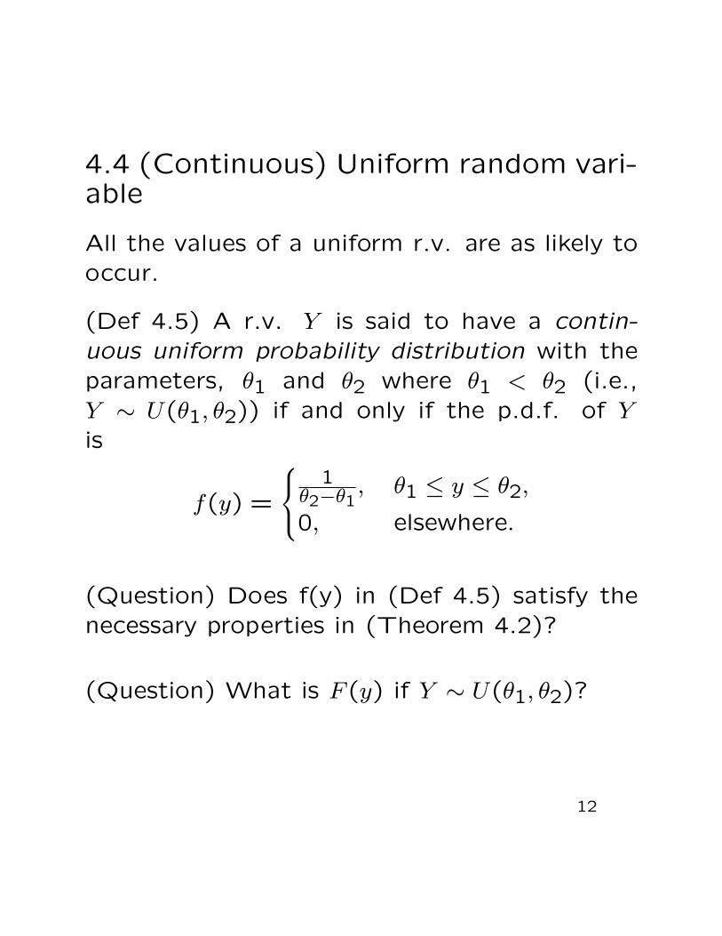
4.4 (Continuous) Uniform random vari-able

All the values of a uniform r.v. are as likely tooccur.

(Def 4.5) A r.v. Y is said to have a contin-uous uniform probability distribution with theparameters, θ1 and θ2 where θ1 < θ2 (i.e.,Y ∼ U(θ1, θ2)) if and only if the p.d.f. of Yis

f(y) =

1

θ2−θ1, θ1 ≤ y ≤ θ2,

0, elsewhere.

(Question) Does f(y) in (Def 4.5) satisfy thenecessary properties in (Theorem 4.2)?

(Question) What is F (y) if Y ∼ U(θ1, θ2)?

12

(Theorem 4.6(p.168))If θ1 < θ2 and Y is a r.v. uniformly distributedon the interval (θ1, θ2). Then

µ = E(Y ) =θ1 + θ2

2and σ2 = V (Y ) =

(θ2 − θ1)2

12

(Proof)

(Exercise 4.51)The cycle time for trucks haul-ing concrete to a highway construction site isuniformly distributed over the interval 50 to 70minutes. What is the probability that the cycletime exceeds 65 minutes if it is known that thecycle time exceeds 55 minutes?

13

4.5 Normal random variable

The most widely used continuous probabilitydistribution is the normal distribution with thefamiliar ‘bell’ shape(the empirical rule(p.10)).

(Def 4.7) A r.v. Y is said to have a normalprobability distribution with two parameters,mean µ and variance σ2 (i.e., Y ∼ N(µ, σ2))if and only if, for σ > 0 and −∞ < µ < ∞, thep.d.f. of Y is

f(y) =1

σ√

2πe−(y−µ)2/(2σ2), −∞ < y <∞

(Question) Does f(y) in (Def 4.7) satisfy thenecessary properties in (Theorem 4.2)?

(Theorem 4.7) If Y is a normally distributedr.v. with parameters µ and σ, then

E(Y ) = µ and V (Y ) = σ2.

[Note] µ(location parameter) locates the center of the

distribution and σ(scale parameter) measures its spread.

14

[Properties of Y ∼ N(µ, σ2)]

• f(y) is symmetric at µ

i) F (µ) = P (Y ≤ µ) = P (Y ≥ µ) = 1− F (µ)=0.5,

ii) For a such that a ≥ 0,

· F (µ− a) = P (Y ≤ µ− a) = P (Y ≥ µ+ a) = 1− F (µ+ a),

· F (µ+ a)− F (µ− a) = P (µ− a < Y < µ+ a)

= 2P (µ < Y < µ+ a) = 2P (µ− a < Y < µ)

So, it is enough to know the areas on only one side

of the mean µ.

(Question) What is F (a) = P (Y ≤ a) if Y ∼N(µ, σ2)?

The calculation of P (Y ≤ a) requires evalua-tion of the integral∫ a

−∞

1

σ√

2πe−(y−µ)2/(2σ2).

Unfortunately, a closed-form expression for thisintegral does not exist. Hence we need the useof numerical integration techniques.

But there is an easy way to do this job: UseTable 4, Appendix III. For the use of Table 4,we need to know the three following steps :

15

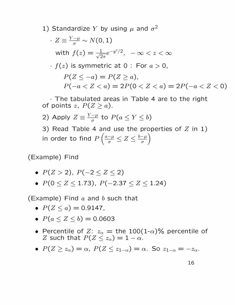
1) Standardize Y by using µ and σ2

· Z ≡ Y−µσ∼ N(0,1)

with f(z) = 1√2πe−y

2/2, −∞ < z <∞

· f(z) is symmetric at 0 : For a > 0,

P (Z ≤ −a) = P (Z ≥ a),

P (−a < Z < a) = 2P (0 < Z < a) = 2P (−a < Z < 0)

· The tabulated areas in Table 4 are to the rightof points z, P (Z ≥ a).

2) Apply Z ≡ Y−µσ

to P (a ≤ Y ≤ b)

3) Read Table 4 and use the properties of Z in 1)

in order to find P(a−µσ≤ Z ≤ b−µ

σ

)(Example) Find

• P (Z > 2), P (−2 ≤ Z ≤ 2)

• P (0 ≤ Z ≤ 1.73), P (−2.37 ≤ Z ≤ 1.24)

(Example) Find a and b such that

• P (Z ≤ a) = 0.9147,

• P (a ≤ Z ≤ b) = 0.0603

• Percentile of Z: zα = the 100(1-α)% percentile ofZ such that P (Z ≤ zα) = 1− α.

• P (Z ≥ zα) = α, P (Z ≤ z1−α) = α. So z1−α = −zα.

16

(Example 4.9)

The achievement scores for a college entranceexamination are normally distributed with mean75 and standard deviation 10. What fractionof the scores lies between 80 and 90?

(Exercise 4.73)

(Example)Let Y ∼ N(3,16).(a) Find P (Y ≤ 5)(b) Find P (Y ≥ 4)(c) Find P (4 ≤ Y ≤ 8)(d) Find the value of c such that P (| Y − 3 |≤c) = 0.9544.

(Example) A candy maker produces mints thathave a label weight of 20.4 grams. Assumingthat the distribution of the weights of thesemints is N(21.37,0.16). Let Y denote the

17

weight of a single mint selected at randomfrom the production line. Find P (Y ≥ 22.07).

4.6 Gamma random variable

[1] The Gamma probability distribution is widelyused in engineering, science, and business, tomodel continuous variables that are always pos-itive and have skewed distributions.

The lengths of time between malfunctions foraircraft engines possess a skewed distributionas do the lengths of time between arrivals ata supermarket checkout queue. The popula-tions associated with theses random variablesfrequently possess distributions that are ade-quately modelled by a gamma density function.

[2] The Gamma probability function providestwo important probability distributions:

• Chi-squared distribution

• Exponential distribution

18

[1](Def 4.8) A r.v. Y is said to have a gammaprobability distribution with parameters α > 0and β > 0 (i.e., Y ∼ gamma(α, β)) if and onlyif the p.d.f. of Y is

f(y) =

yα−1e−y/β

βαΓ(α) 0 ≤ y <∞,0 elsewhere.

where Γ(α) =∫∞0 yα−1e−ydy.

Note that

· Γ(α) : the gamma function,Γ(α+ 1) = αΓ(α) where α > 0,Γ(1) = 1, Γ(n+ 1) = n! for any integer n > 0.

· α is the shape parameter and β is the scale pa-rameter

(Question) Does f(y) in (Def 4.8) satisfy thenecessary properties in (Theorem 4.2)?

(Theorem 4.8) If Y is a gamma distributionwith parameters α and β, then

µ = E(Y ) = αβ and σ2 = V (Y ) = αβ2.

19

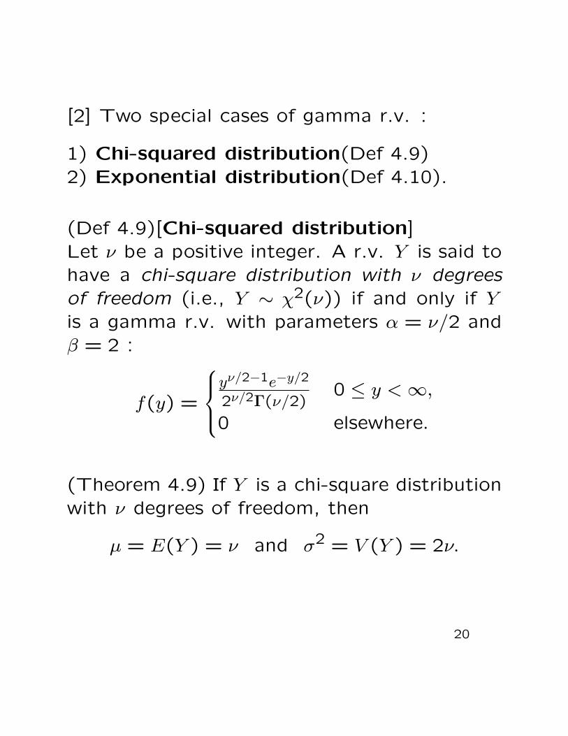
[2] Two special cases of gamma r.v. :

1) Chi-squared distribution(Def 4.9)2) Exponential distribution(Def 4.10).

(Def 4.9)[Chi-squared distribution]Let ν be a positive integer. A r.v. Y is said tohave a chi-square distribution with ν degreesof freedom (i.e., Y ∼ χ2(ν)) if and only if Yis a gamma r.v. with parameters α = ν/2 andβ = 2 :

f(y) =

yν/2−1e−y/2

2ν/2Γ(ν/2)0 ≤ y <∞,

0 elsewhere.

(Theorem 4.9) If Y is a chi-square distributionwith ν degrees of freedom, then

µ = E(Y ) = ν and σ2 = V (Y ) = 2ν.

20

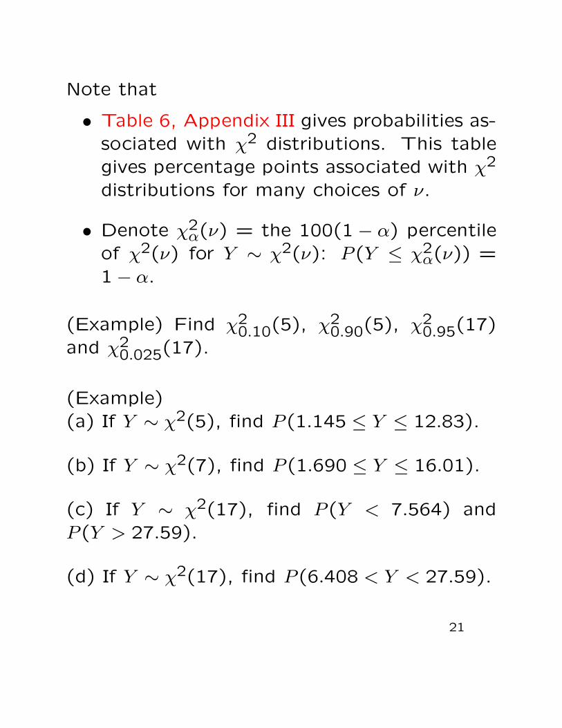
Note that

• Table 6, Appendix III gives probabilities as-sociated with χ2 distributions. This tablegives percentage points associated with χ2

distributions for many choices of ν.

• Denote χ2α(ν) = the 100(1− α) percentile

of χ2(ν) for Y ∼ χ2(ν): P (Y ≤ χ2α(ν)) =

1− α.

(Example) Find χ20.10(5), χ2

0.90(5), χ20.95(17)

and χ20.025(17).

(Example)(a) If Y ∼ χ2(5), find P (1.145 ≤ Y ≤ 12.83).

(b) If Y ∼ χ2(7), find P (1.690 ≤ Y ≤ 16.01).

(c) If Y ∼ χ2(17), find P (Y < 7.564) andP (Y > 27.59).

(d) If Y ∼ χ2(17), find P (6.408 < Y < 27.59).

21

(Def 4.10)[Exponential distribution]A r.v. Y is said to have an exponential distri-bution with parameter β > 0 (i.e., Y ∼ exp(β))if and only if the density function of Y is

f(y) =

1βe−y/β 0 ≤ y <∞,

0 elsewhere.

[Note] The gamma density function in which α = 1 is

called the exponential density function.

(Theorem 4.10) If Y is an exponential randomvariable with parameter β, then

µ = E(Y ) = β and σ2 = V (Y ) = β2.

Note that

• The exponential density function is usefulfor modelling the length of life of electroniccomponents.

• The memoryless property of the exponen-tial distribution :

P (Y > a+b | Y > a) = P (Y > b) for a, b > 0

22

(Example) Let Y have an exponential distribu-tion with mean=40. Find(a) probability density function of Y .(b) P (Y < 36)(c) P (Y > 36 | Y > 30)

(Exercise 4.93)Times between accidents for allfatal accidents on scheduled American domes-tic passenger flights during the years 1948 through1961 were found to have an approximately ex-ponential distribution with mean 44 days.

a. If one of the accidents occurred on July 1 ofa randomly selected year in the study period,what is the probability that another accidentoccurred that same month?

b. What is the variance of the times betweenaccidents for the years just indicated?

23

(Exercise 4.110)If Y has a probability densityfunction given by

f(y) =

4y2e−2y 0 ≤ y <∞,0 elsewhere.

Obtain E(Y) and V(Y).

(EXAMPLE 4.11)A gasoline wholesale distrib-utor has bulk storage tanks that hold fixed sup-plies and are filled every Monday. Of interest tothe wholesaler is the proportion of this supplythat is sold during the week. Over many weeksof observation, the distributor found that thisproportion could be modeled by a beta distri-bution with = 4 and = 2. Find the probabilitythat the wholesaler will sell at least 90week.

4.10 Tchebysheff’s Theorem (See 3.11)

(Theorem 4.13) Let Y be a r.v. with finitemean µ and variance σ2. Then, for any k > 0,

P (| Y − µ |< kσ) ≥ 1−1

k2or P (| Y − µ |≥ kσ) ≤

1

k2

(Example 4.17)

(Exercise 4.147) A machine used to fill ce-real boxes dispenses, on the average, µ ouncesper box. The manufacturer wants the actualounces dispensed Y to be within 1 ounce of µat least 75% of the time. What is the largestvalue of σ, the standard deviation of Y , thatcan be tolerated if the manufacturer’s objec-tives are to be met?

24