Chapter 4Displaying and Summarizing

Quantitative Data

Display: Histograms, Stem and Leaf Plots

Numerical Summaries: Median, Mean, Quartiles, Standard Deviation

Relative Frequency Histogram of Exam Grades

0.05

.10

.15

.20

.25

.30

40 50 60 70 80 90Grade

Rel

ativ

e fr

eque

ncy

100

Frequency HistogramsBAKER CITY HOSPITAL - LENGTH OF STAY

DISTRIBUTION

0

10

20

30

40

50

60

70

0<2 2<4 4<6 6<8 8<10 10<12 12<14 14<16 16<18

Frequency Histograms

A histogram shows three general types of information:

It provides visual indication of where the approximate center of the data is.

We can gain an understanding of the degree of spread, or variation, in the data.

We can observe the shape of the distribution.

All 200 m Races 20.2 secs or less

Histograms Showing Different Centers

0

10

20

30

40

50

60

70

0<2 2<4 4<6 6<8 8<10 10<12 12<14 14<16 16<18

0

10

20

30

40

50

60

70

0<2 2<4 4<6 6<8 8<10 10<12 12<14 14<16 16<18

Histograms - Same Center, Different Spread

0

10

20

30

40

50

60

70

0<2

2<4

4<6

6<8

8<10

10<12

12<14

14<16

16<18

0

10

20

30

40

50

60

70

0<2 2<4 4<6 6<8 8<10 10<12 12<14 14<16 16<18

Frequency and Relative Frequency Histograms

identify smallest and largest values in data set

divide interval between largest and smallest values into between 5 and 20 subintervals called classes

* each data value in one and only one class

* no data value is on a boundary

How Many Classes?

3333.2

formulastwofrom chooseCan

n

size sample theis

)2log(

)log(1

:Rule Sturges'

n

n

Histogram Construction (cont.)* compute frequency or relative frequency of observations in each class

* x-axis: class boundaries;

y-axis: frequency or relative frequency scale

* over each class draw a rectangle with height corresponding to the frequency or relative frequency in that class

Example. Number of daily employee absences from work

106 obs; approx. no of classes=

{2(106)}1/3 = {212}1/3 = 5.69

1+ log(106)/log(2) = 1 + 6.73 = 7.73 There is no single “correct” answer for

the number of classes For example, you can choose 6, 7, 8, or

9 classes; don’t choose 15 classes

EXCEL Histogram

Absences from Work (cont.) 6 classes class width: (158-121)/6=37/6=6.17 7 6 classes, each of width 7; classes span

6(7)=42 units data spans 158-121=37 units classes overlap the span of the actual

data values by 42-37=5 lower boundary of 1st class: (1/2)(5)

units below 121 = 121-2.5 = 118.5

EXCEL histogram

Grades on a statistics exam

Data:

75 66 77 66 64 73 91 65 59 86 61 86 61

58 70 77 80 58 94 78 62 79 83 54 52 45

82 48 67 55

Frequency Distribution of Grades

Class Limits Frequency40 up to 50

50 up to 60

60 up to 70

70 up to 80

80 up to 90

90 up to 100

Total

2

6

8

7

5

2

30

Relative Frequency Distribution of Grades

Class Limits Relative Frequency40 up to 50

50 up to 60

60 up to 70

70 up to 80

80 up to 90

90 up to 100

2/30 = .067

6/30 = .200

8/30 = .267

7/30 = .233

5/30 = .167

2/30 = .067

Relative Frequency Histogram of Grades

0.05

.10

.15

.20

.25

.30

40 50 60 70 80 90Grade

Rel

ativ

e fr

eque

ncy

100

Based on the histo-gram, about what percent of the values are between 47.5 and 52.5?

1 2 3 4

0% 0%0%0%

1. 50%

2. 5%

3. 17%

4. 30%

CountdownCountdown

10

Stem and leaf displays Have the following general appearance

stem leaf

1 8 9

2 1 2 8 9 9

3 2 3 8 9

4 0 1

5 6 7

6 4

Stem and Leaf Displays Partition each no. in data into a “stem” and

“leaf” Constructing stem and leaf display

1) deter. stem and leaf partition (5-20 stems)

2) write stems in column with smallest stem at top; include all stems in range of data

3) only 1 digit in leaves; drop digits or round off

4) record leaf for each no. in corresponding stem row; ordering the leaves in each row helps

Example: employee ages at a small company

18 21 22 19 32 33 40 41 56 57 64 28 29 29 38 39; stem: 10’s digit; leaf: 1’s digit

18: stem=1; leaf=8; 18 = 1 | 8

stem leaf

1 8 9

2 1 2 8 9 9

3 2 3 8 9

4 0 1

5 6 7

6 4

Suppose a 95 yr. old is hiredstem leaf

1 8 9

2 1 2 8 9 9

3 2 3 8 9

4 0 1

5 6 7

6 4

7

8

9 5

Number of TD passes by NFL teams: 2010 season

(stems are 10’s digit)

stem leaf

3 011337

2 5566667889

2 0123444

1 03447889

0 9

Pulse Rates n = 138

# Stem Leaves 4* 3 4. 588 9 5* 001233444 10 5. 5556788899 23 6* 00011111122233333344444 23 6. 55556666667777788888888 16 7* 00000112222334444 23 7. 55555666666777888888999 10 8* 0000112224 10 8. 5555667789 4 9* 0012 2 9. 58 4 10* 0223 10. 1 11* 1

Advantages/Disadvantages of Stem-and-Leaf Displays

Advantages

1) each measurement displayed

2) ascending order in each stem row

3) relatively simple (data set not too large) Disadvantages

display becomes unwieldy for large data sets

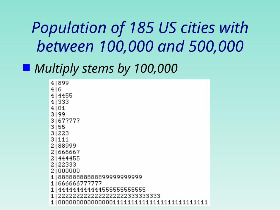
Population of 185 US cities with between 100,000 and 500,000

Multiply stems by 100,000

Back-to-back stem-and-leaf displays. TD passes by NFL teams: 1999, 2009multiply stems by 10

1999 2009

2 4

6 3

2 3 0444

6655 2 6677788899

43322221100 2 011113

9998887666 1 55666788

421 1 0122

Below is a stem-and-leaf display for the pulse rates of 24 women at a health clinic. How many pulses are between 67 and 77?

Stems are 10’s digits

1 2 3 4 5

0% 0% 0%0%0%

1. 4

2. 6

3. 8

4. 10

5. 12 CountdownCountdown

10

Interpreting Graphical Displays: Shape

A distribution is symmetric if the right and left

sides of the histogram are approximately mirror

images of each other.

Symmetric distribution

Complex, multimodal distribution

Not all distributions have a simple overall shape,

especially when there are few observations.

Skewed distribution

A distribution is skewed to the right if the right

side of the histogram (side with larger values)

extends much farther out than the left side. It is

skewed to the left if the left side of the histogram

extends much farther out than the right side.

Shape (cont.)Female heart attack patients in New York state

Age: left-skewed Cost: right-skewed

Alaska Florida

Shape (cont.): Outliers

An important kind of deviation is an outlier. Outliers are observations

that lie outside the overall pattern of a distribution. Always look for

outliers and try to explain them.

The overall pattern is fairly

symmetrical except for 2

states clearly not belonging

to the main trend. Alaska

and Florida have unusual

representation of the

elderly in their population.

A large gap in the

distribution is typically a

sign of an outlier.

Center: typical value of frozen personal pizza? ~$2.65

Spread: fuel efficiency 4, 8 cylinders

4 cylinders: more spread 8 cylinders: less spread

Other Graphical Methods for Economic Data

Time plots

plot observations in time order, with time on the horizontal axis and the vari-able on the vertical axis

** Time series

measurements are taken at regular intervals (monthly unemployment, quarterly GDP, weather records, electricity demand, etc.)

Unemployment Rate, by Educational Attainment

Water Use During Super Bowl

Winning Times 100 M Dash

Annual Mean Temperature

End of Histograms, Stem and Leaf plots

Describing Distributions Numerically:

Medians and Quartiles

2 characteristics of a data set to measure

center

measures where the “middle” of the data is located

variability

measures how “spread out” the data is

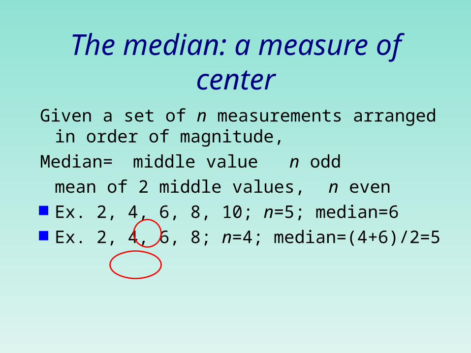
The median: a measure of center

Given a set of n measurements arranged in order of magnitude,

Median= middle value n odd

mean of 2 middle values, n even

Ex. 2, 4, 6, 8, 10; n=5; median=6 Ex. 2, 4, 6, 8; n=4; median=(4+6)/2=5

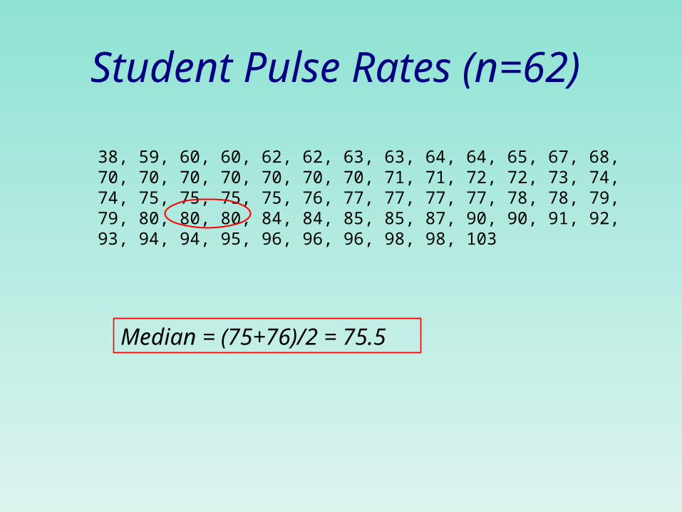
Student Pulse Rates (n=62)

38, 59, 60, 60, 62, 62, 63, 63, 64, 64, 65, 67, 68, 70, 70, 70, 70, 70, 70, 70, 71, 71, 72, 72, 73, 74, 74, 75, 75, 75, 75, 76, 77, 77, 77, 77, 78, 78, 79, 79, 80, 80, 80, 84, 84, 85, 85, 87, 90, 90, 91, 92, 93, 94, 94, 95, 96, 96, 96, 98, 98, 103

Median = (75+76)/2 = 75.5

Medians are used often

Year 2011 baseball salaries

Median $1,450,000 (max=$32,000,000 Alex Rodriguez; min=$414,000)

Median fan age: MLB 45; NFL 43; NBA 41; NHL 39

Median existing home sales price: May 2011 $166,500; May 2010 $174,600

Median household income (2008 dollars) 2009 $50,221; 2008 $52,029

The median splits the histogram into 2 halves of equal area

Examples Example: n = 7

17.5 2.8 3.2 13.9 14.1 25.3 45.8 Example n = 7 (ordered): 2.8 3.2 13.9 14.1 17.5 25.3 45.8 Example: n = 8

17.5 2.8 3.2 13.9 14.1 25.3 35.7 45.8 Example n =8 (ordered)

2.8 3.2 13.9 14.1 17.5 25.3 35.7 45.8

m = 14.1

m = (14.1+17.5)/2 = 15.8

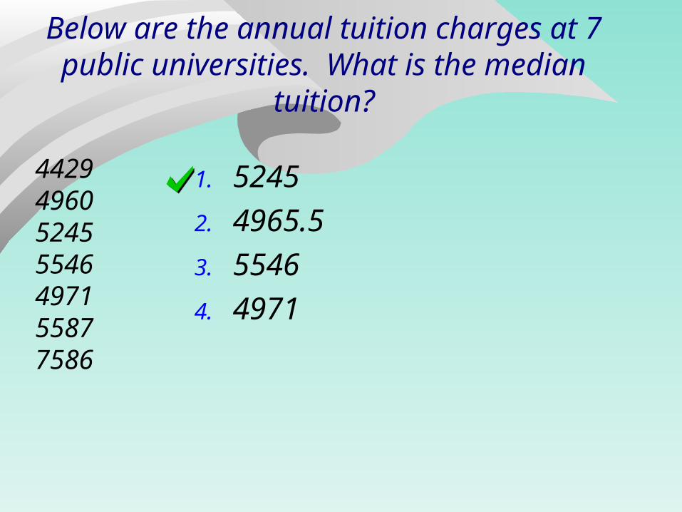
Below are the annual tuition charges at 7 public universities. What is the median

tuition?

4429496049604971524555467586

1. 5245

2. 4965.5

3. 4960

4. 4971

Below are the annual tuition charges at 7 public universities. What is the median

tuition?

4429496052455546497155877586

1. 5245

2. 4965.5

3. 5546

4. 4971

Measures of Spread

The range and interquartile range

Ways to measure variability

range=largest-smallest OK sometimes; in general, too crude;

sensitive to one large or small data value

The range measures spread by examining the ends of the data

A better way to measure spread is to examine the middle portion of the data

m = median = 3.4

Q1= first quartile = 2.3

Q3= third quartile = 4.2

1 1 0.62 2 1.23 3 1.64 4 1.95 5 1.56 6 2.17 7 2.38 6 2.39 5 2.510 4 2.811 3 2.912 2 3.313 1 3.414 2 3.615 3 3.716 4 3.817 5 3.918 6 4.119 7 4.220 6 4.521 5 4.722 4 4.923 3 5.324 2 5.625 1 6.1

Quartiles: Measuring spread by examining the middle

The first quartile, Q1, is the value in the

sample that has 25% of the data at or

below it (Q1 is the median of the lower

half of the sorted data).

The third quartile, Q3, is the value in the

sample that has 75% of the data at or

below it (Q3 is the median of the upper

half of the sorted data).

Quartiles and median divide data into 4 pieces

Q1 M Q3Q1 M Q3

1/41/4 1/41/4 1/41/4 1/41/4

Quartiles are common measures of spread

http://www2.acs.ncsu.edu/UPA/admissions/fresprof.htm

http://www2.acs.ncsu.edu/UPA/peers/current/ncsu_peers/sat.htm

University of Southern California

UNC-CH

Rules for Calculating QuartilesStep 1: find the median of all the data (the median divides the data in half)

Step 2a: find the median of the lower half; this median is Q1;Step 2b: find the median of the upper half; this median is Q3.

Important:when n is odd include the overall median in both halves;when n is even do not include the overall median in either half.

Example 2 4 6 8 10 12 14 16 18 20 n = 10

Median m = (10+12)/2 = 22/2 = 11

Q1 : median of lower half 2 4 6 8 10

Q1 = 6

Q3 : median of upper half 12 14 16 18 20

Q3 = 16

11

Pulse Rates n = 138

# Stem Leaves4*

3 4. 5889 5* 00123344410 5. 555678889923 6* 0001111112223333334444423 6. 5555666666777778888888816 7* 0000011222233444423 7. 5555566666677788888899910 8* 000011222410 8. 55556677894 9* 00122 9. 584 10* 0223

10.1 11* 1

Median: mean of pulses in locations 69 & 70: median= (70+70)/2=70

Q1: median of lower half (lower half = 69 smallest pulses); Q1 = pulse in ordered position 35;Q1 = 63

Q3 median of upper half (upper half = 69 largest pulses); Q3= pulse in position 35 from the high end; Q3=78

Below are the weights of 31 linemen on the NCSU football team. What is the

value of the first quartile Q1?

# stemleaf

2 2255

4 2357

6 2426

7 257

10 26257

12 2759

(4) 281567

15 2935599

10 30333

7 3145

5 32155

2 336

1 340

1 2. 3. 4.

0% 0%0%0%

1. 287

2. 257.5

3. 263.5

4. 262.5

CountdownCountdown

10

Interquartile range

lower quartile Q1

middle quartile: median upper quartile Q3

interquartile range (IQR)IQR = Q3 – Q1

measures spread of middle 50% of the data

Example: beginning pulse rates

Q3 = 78; Q1 = 63

IQR = 78 – 63 = 15

Below are the weights of 31 linemen on the NCSU football team. The first quartile Q1 is 263.5. What is the value of the IQR?

# stemleaf

2 2255

4 2357

6 2426

7 257

10 26257

12 2759

(4) 281567

15 2935599

10 30333

7 3145

5 32155

2 336

1 340

1. 2. 3 4.

0% 0%0%0%

1. 23.5

2. 39.5

3. 46

4. 69.5

CountdownCountdown

10

5-number summary of data

Minimum Q1 median Q3 maximum

Pulse data

45 63 70 78 111

End of Medians and Quartiles

Numerical Summaries of Symmetric Data.

Measure of Center: Mean

Measure of Variability: Standard Deviation

Symmetric DataBody temp. of 93 adults

Recall: 2 characteristics of a data set to measure

center

measures where the “middle” of the data is located

variability

measures how “spread out” the data is

Measure of Center When Data Approx. Symmetric

mean (arithmetic mean) notationx i

x x x x

n

x x x x x

i

n

ii

n

n

: th measurement in a set of observations

number of measurements in data set; sample

size

1 2 3

11 2 3

, , , ,

:

N

x

n

x

n

xxxxx

x

N

ii

n

ii

n

1

1321

size population = N

known)not typically(value mean Population

mean Sample

Connection Between Mean and Histogram

A histogram balances when supported at the mean. Mean x = 140.6

Histogram

0

10

20

30

40

50

60

70

118.

5

125.

5

132.

5

139

.5

146.

5

153.

5

160

.5

Mor

e

Absences from Work

Fre

qu

en

cy

Frequency

Mean: balance pointMedian: 50% area each half

right histo: mean 55.26 yrs, median 57.7yrs

Properties of Mean, Median1.The mean and median are unique; that is, a

data set has only 1 mean and 1 median (the mean and median are not necessarily equal).

2.The mean uses the value of every number in the data set; the median does not.

14

20 4 6Ex. 2, 4, 6, 8. 5; 5

4 2

21 4 6Ex. 2, 4, 6, 9. 5 ; 5

4 2

x m

x m

Example: class pulse rates

53 64 67 67 70 76 77 77 78 83 84 85 85 89 90 90 90 90 91 96 98 103 140

23

1

23

84.48;23

:location: 12th obs. 85

ii

n

xx

m m

2010, 2011 baseball salaries

2010

n = 845

= $3,297,828

median = $1,330,000

max = $33,000,000

2011

n = 848

= $3,305,393

median = $1,450,000

max = $32,000,000

Disadvantage of the mean

Can be greatly influenced by just a few observations that are much greater or much smaller than the rest of the data

Mean, Median, Maximum BB Salaries

Baseball Salaries: Mean, Median and Maximum 1985-2006

200,000

700,000

1,200,000

1,700,000

2,200,000

2,700,000

3,200,000

1985

1987

1989

1991

1993

1995

1997

1999

2001

2003

2005

Year

Mea

n, M

edia

n S

alar

y

0

5,000,000

10,000,000

15,000,000

20,000,000

25,000,000

30,000,000

Max

imu

m S

alar

y

Mean Median Maximum

Skewness: comparing the mean, and median

Skewed to the right (positively skewed) mean>median

53

490

102 7235 21 26 17 8 10 2 3 1 0 0 1

0

100

200

300

400

500

600

Freq

uenc

y

Salary ($1,000's)

2011 Baseball Salaries

Skewed to the left; negatively skewed

Mean < median mean=78; median=87;

Histogram of Exam Scores

0

10

20

30

20 30 40 50 60 70 80 90 100Exam Scores

Fre

qu

en

cy

Symmetric data

mean, median approx. equal

Bank Customers: 10:00-11:00 am

0

5

10

15

20

Number of Customers

Fre

qu

en

cy

DESCRIBING VARIABILITY OF SYMMETRIC DATA

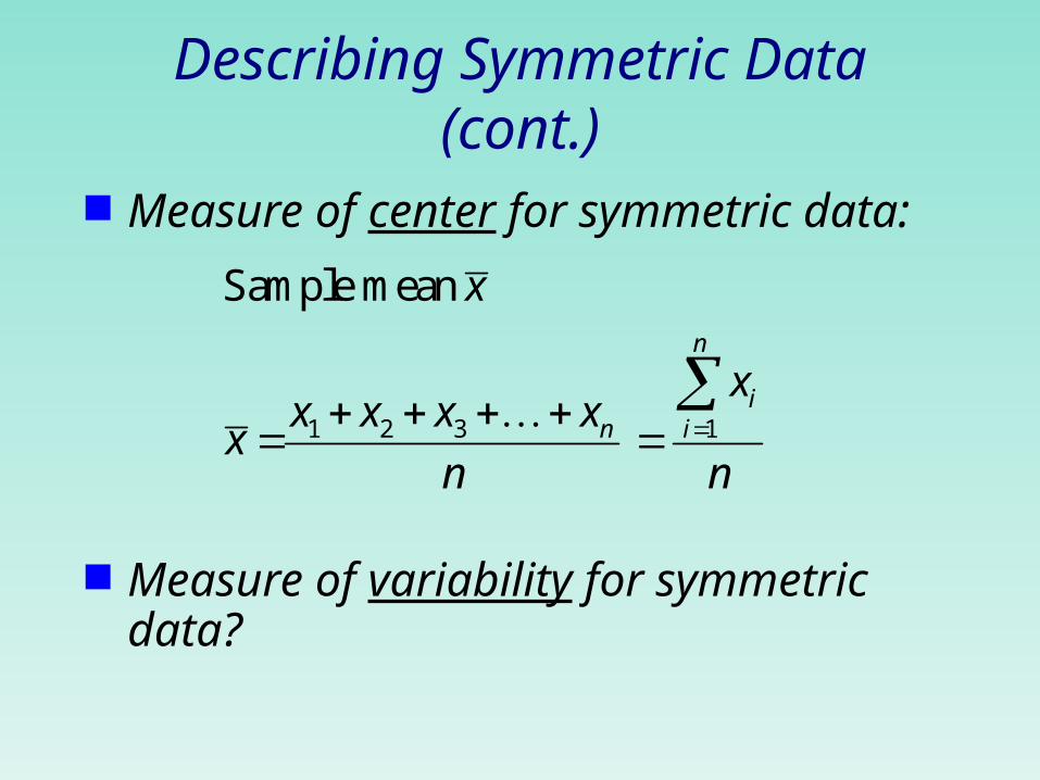
Describing Symmetric Data (cont.)

Measure of center for symmetric data:

Measure of variability for symmetric data?

1 2 3 1

Sample mean n

in i

x

xx x x x

xn n

Example

2 data sets:

x1=49, x2=51 x=50

y1=0, y2=100 y=50

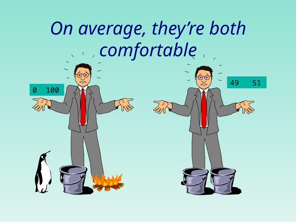
On average, they’re both comfortable

0 10049 51

Ways to measure variability

1. range=largest-smallest

ok sometimes; in general, too crude; sensitive to one large or small obs.

1

2. measure spread from the middle, where

the middle is the mean ;

deviation of from the mean:

( ); sum the deviations of all the 's from ;

i i

n

i ii

x

x x x

x x x x

1

( ) 0 always; tells us nothingn

ii

x x

Previous Example

1 2

1 2

1 2

1 2

sum of deviations from mean:

49, 51; 50

( ) ( ) (49 50) (51 50) 1 1 0;

0, 100; 50

( ) ( ) (0 50) (100 50) 50 50 0

x x x

x x x x

y y y

y y y y

The Sample Standard Deviation, a measure of spread around the mean Square the deviation of each

observation from the mean; find the square root of the “average” of these squared deviations

deviation

standard sample thecalled1

)(

average theofroot square thethen take

,average"" thefind and)(;)(

1

2

1

22

n

xxs

xxxx

n

ii

n

iii

Calculations …

Mean = 63.4

Sum of squared deviations from mean = 85.2

(n − 1) = 13; (n − 1) is called degrees freedom (df)

s2 = variance = 85.2/13 = 6.55 inches squared

s = standard deviation = √6.55 = 2.56 inches

Women height (inches)

x

x

2

1

2 )(1

1xx

ns

n

i

1. First calculate the variance s2.2. Then take the square root to get the

standard deviation s.

2

1

)(1

1xx

ns

n

i

Mean± 1 s.d.

We’ll never calculate these by hand, so make sure to know how to get the standard deviation using your calculator, Excel, or other software.

Population Standard Deviation

2

1

( )population standard deviation

value of typically not known;

use to estimate value of

N

ii

x

N

s

Remarks

1. The standard deviation of a set of measurements is an estimate of the likely size of the chance error in a single measurement

Remarks (cont.)

2. Note that s and are always greater than or equal to zero.

3. The larger the value of s (or ), the greater the spread of the data.

When does s=0? When does =0?When all data values are the same.

Remarks (cont.)4. The standard deviation is the most

commonly used measure of risk in finance and business– Stocks, Mutual Funds, etc.

5. Variance s2 sample variance 2 population variance Units are squared units of the original data square $, square gallons ??

Remarks 6):Why divide by n-1 instead of n?

degrees of freedom each observation has 1 degree of

freedom however, when estimate unknown

population parameter like , you lose 1 degree of freedom

1

)(; of value

unkown theestimate to use we,for formulaIn

1

2

n

xxs

xs

n

ii

Remarks 6) (cont.):Why divide by n-1 instead of n? Example

Suppose we have 3 numbers whose average is 9

x1= x2=

then x3 must be

once we selected x1 and x2, x3 was determined since the average was 9

3 numbers but only 2 “degrees of freedom”

Since the average (mean) is 9, x1 + x2 + x3 must equal 9*3 = 27, so x3 = 27 – (x1 + x2)

Choose ANY values for x1 and x2

Computational Example

67.11

;42.367.113

35

3

25.2025.25.225.12

3

)5.4()5(.)5.1()5.3(

14

)5.49()5.45()5.43()5.41(

5.4;9,5,3,1

2

2222

2222

418

s

s

xnsobservatio

class pulse rates

2 2

53 64 67 67 70 76 77 77 78 83 84 85 85 89 90

90 90 90 91 96 98 103 140

23 84.48 85

290.26(beats per minute)

17.037 beats per minute

n x m

s

s

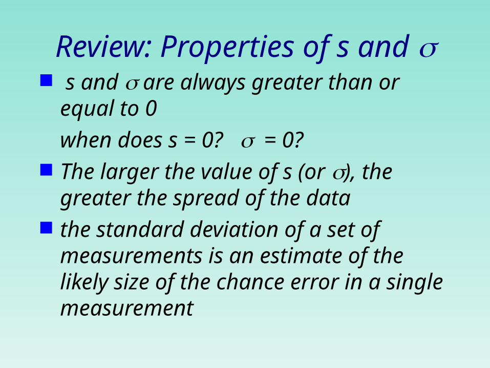
Review: Properties of s and s and are always greater than or

equal to 0

when does s = 0? = 0? The larger the value of s (or ), the

greater the spread of the data the standard deviation of a set of

measurements is an estimate of the likely size of the chance error in a single measurement

Summary of Notation

2

SAMPLE

sample mean

sample median

sample variance

sample stand. dev.

y

m

s

s

2

POPULATION

population mean

population median

population variance

population stand. dev.

m

End of Chapter 4