chapter 4: fluid kinematics - unige.it dei fluidi i 8 chapter 4: fluid kinematics ... airplane...

Chapter 4: Fluid Kinematics

Chapter 4: Fluid Kinematics Meccanica dei Fluidi I 2

Overview

Fluid kinematics deals with the motion of fluids without considering the forces and moments which create the motion.

Items discussed in this Chapter.

Material derivative and its relationship to Lagrangian and Eulerian descriptions of fluid flow.

Fundamental kinematic properties of fluid motion and deformation.

Reynolds Transport Theorem.


Lagrangian Description

Lagrangian description of fluid flow tracks the position and velocity of individual particles.

Based upon Newton's laws of motion.

Difficult to use for practical flow analysis. Fluids are composed of billions of molecules.

Interaction between molecules hard to describe/model.

However, useful for specialized applications Sprays, particles, bubble dynamics, rarefied gases.

Coupled Eulerian-Lagrangian methods.

Named after Italian mathematician Joseph Louis Lagrange (1736-1813).


Eulerian Description

Eulerian description of fluid flow: a flow domain or control volume is defined by which fluid flows in and out.

We define field variables which are functions of space and time.

Pressure field, P = P(x,y,z,t)

Velocity field,

Acceleration field,

These (and other) field variables define the flow field.

Well suited for formulation of initial boundary-value problems (PDE's).

Named after Swiss mathematician Leonhard Euler (1707-1783).

, , , , , , , , ,V u x y z t i v x y z t j w x y z t k

, , , , , , , , ,x y za a x y z t i a x y z t j a x y z t k

, , ,a a x y z t

, , ,V V x y z t


Example: Coupled Eulerian-Lagrangian

Method

Forensic analysis of Columbia accident: simulation of

shuttle debris trajectory using Eulerian CFD for flow field

and Lagrangian method for the debris.


Acceleration Field

Consider a fluid particle and Newton's second law,

The acceleration of the particle is the time derivative of

the particle's velocity:

However, particle velocity at a point is the same as the

fluid velocity,

To take the time derivative, chain rule must be used.

particle particle particleF m a

particle

particle

dVa

dt

, ,particle particle particle particleV V x t y t z t

particle particle particle

particle

dx dy dzV dt V V Va

t dt x dt y dt z dt

, t)


Acceleration Field

Since

In vector form, the acceleration can be written as

First term is called the local acceleration and is nonzero only for unsteady flows.

Second term is called the advective (or convective) acceleration and accounts for the effect of the fluid particle moving to a new location in the flow, where the velocity is different (it can thus be nonzero even for steady flows).

, , ,dV V

a x y z t V Vdt t

particle

V V V Va u v w

t x y z

, ,particle particle particledx dy dz

u v wdt dt dt

. .


Material Derivative

The total derivative operator d/dt is call the material derivative and is often given special notation, D/Dt.

Advective acceleration is nonlinear: source of many phenomena and primary challenge in solving fluid flow problems.

Provides “transformation”' between Lagrangian and Eulerian frames.

Other names for the material derivative include: total, particle, Lagrangian, Eulerian, and substantial derivative.

DV dV V

V VDt dt t

. .


Flow Visualization

Flow visualization is the visual examination of flow-field features.

Important for both physical experiments and numerical (CFD) solutions.

Numerous methods Streamlines and streamtubes

Pathlines

Streaklines

Timelines

Refractive flow visualization techniques

Surface flow visualization techniques


Streamlines and streamtubes

A streamline is a curve that is

everywhere tangent to the

instantaneous local velocity vector.

Consider an infinitesimal arc length

along a streamline:

By definition must be parallel to

the local velocity vector

Geometric arguments result in the

equation for a streamline

dr dxi dyj dzk

dr

V ui vj wk

dr dx dy dz

V u v w



NASCAR surface pressure contours

and streamlines

Airplane surface pressure contours,

volume streamlines, and surface

streamlines



A streamtube consists of a bundle of

individual streamlines. Since fluid

cannot cross a streamline (by

definition), fluid within a streamtube

must remain there. Streamtubes are,

obviously, instantaneous quantities

and they may change significantly with

time.

In the converging portion of an

incompressible flow field, the

diameter of the streamtube must

decrease as the velocity

increases, so as to conserve

mass.


Pathlines

A pathline is the actual path traveled by an individual fluid particle over some time period.

Same as the fluid particle's material position vector

Particle location at time t:

Particle Image Velocimetry (PIV) is a modern experimental technique to measure velocity field over a plane in the flow field.

, ,particle particle particlex t y t z t

start

t

start

t

x x Vdt


Streaklines

A streakline is the locus

of fluid particles that have

passed sequentially

through a prescribed

point in the flow.

Easy to generate in

experiments: continuous

introduction of dye (in a

water flow) or smoke (in

an airflow) from a point.


Comparisons

If the flow is steady, streamlines, pathlines

and streaklines are identical.

For unsteady flows, they can be very

different.

Streamlines provide an instantaneous

picture of the flow field

Pathlines and streaklines are flow patterns

that have a time history associated with them.


Timelines

A timeline is a set of

adjacent fluid particles

that were marked at

the same (earlier) instant

in time.

Experimentally, timelines

can be generated using a

hydrogen bubble wire: a

line is marked and its

movement/deformation

is followed in time.


Plots of Data

A Profile plot indicates how the value of a scalar property varies along some desired direction in the flow field.

A Vector plot is an array of arrows indicating the magnitude and direction of a vector property at an instant in time.

A Contour plot shows curves of constant values of a scalar property (or magnitude for a vector property) at an instant in time.


Kinematic Description

In fluid mechanics (as in solid mechanics), an element may undergo four fundamental types of motion. a) Translation

b) Rotation

c) Linear strain

d) Shear strain

Because fluids are in constant motion, motion and deformation is best described in terms of rates a) velocity: rate of translation

b) angular velocity: rate of rotation

c) linear strain rate: rate of linear strain

d) shear strain rate: rate of shear strain


Rate of Translation and Rotation

To be useful, these deformation rates must be expressed

in terms of velocity and derivatives of velocity

The rate of translation vector is described

mathematically as the velocity vector.

In Cartesian coordinates:

Rate of rotation (angular velocity)

at a point is defined as the average

rotation rate of two lines which are

initially perpendicular and that

intersect at that point.

V ui vj wk


Rate of Rotation

In 2D the average rotation angle of the

fluid element about the point P is

w = (aa + ab)/2

The rate of rotation of the fluid element

about P is

1 1 1

2 2 2

w v u w v ui j k

y z z x x yw

1 1 1

2 2 2

w v u w v ui j k

y z z x x yw

w

In 3D the angular velocity vector is:

a


Linear Strain Rate

Linear Strain Rate is defined as the rate of increase in length per unit length.

In Cartesian coordinates

The rate of increase of volume of a fluid element per unit volume is the volumetric strain rate, in Cartesian coordinates:

(we are talking about a material volume, hence the D)

Since the volume of a fluid element is constant for an incompressible flow, the volumetric strain rate must be zero.

, ,xx yy zz

u v w

x y z

1xx yy zz

DV u v w

V Dt x y z


Shear Strain Rate

Shear Strain Rate at a point is defined as half the

rate of decrease of the angle between two initially

perpendicular lines that intersect at a point.

positive shear strain

negative shear strain


Shear Strain Rate

The shear strain at point P

is xy = - _ __

aa-b

Shear strain rate can be

expressed in Cartesian

coordinates as:

1 1 1, ,

2 2 2xy zx yz

u v w u v w

y x x z z y

1

2

d

dt


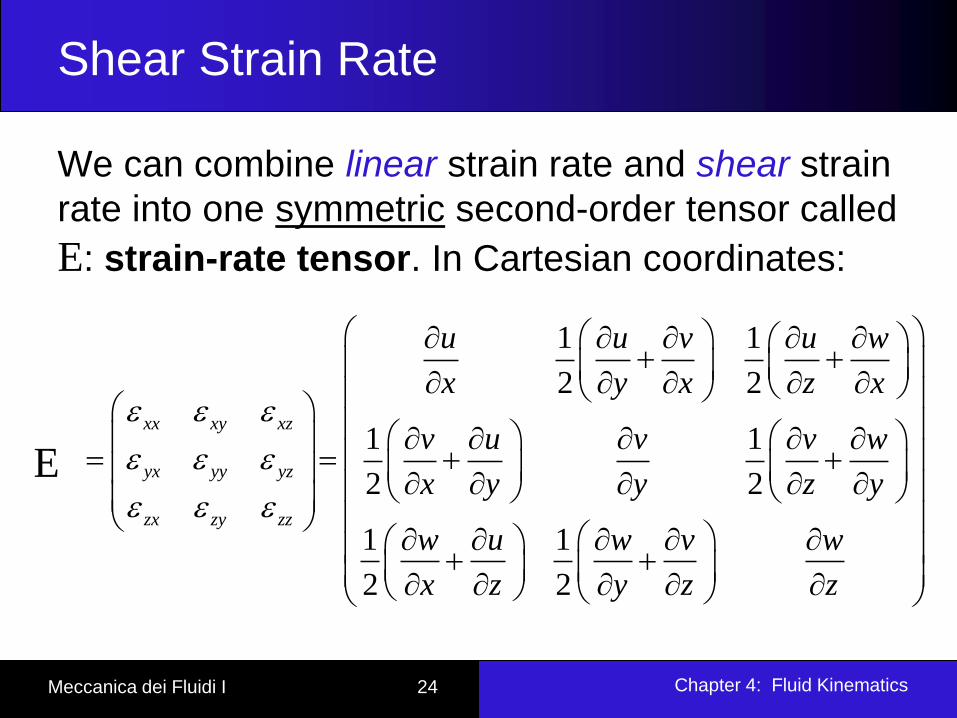
Shear Strain Rate

We can combine linear strain rate and shear strain

rate into one symmetric second-order tensor called

E: strain-rate tensor. In Cartesian coordinates:

1 1

2 2

1 1

2 2

1 1

2 2

xx xy xz

ij yx yy yz

zx zy zz

u u v u w

x y x z x

v u v v w

x y y z y

w u w v w

x z y z z

E


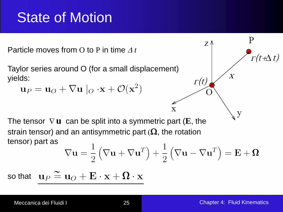
State of Motion

Particle moves from O to P in time D t

Taylor series around O (for a small displacement)

yields:

The tensor u can be split into a symmetric part (E, the

strain tensor) and an antisymmetric part W, the rotation

tensor part as

so that


Shear Strain Rate

Purpose of our discussion of fluid element kinematics:

Better appreciation of the inherent complexity of fluid dynamics

Mathematical sophistication required to fully describe fluid motion

Strain-rate tensor is important for numerous reasons. For example,

Develop relationships between fluid stress and strain rate.

Feature extraction and flow visualization in CFD simulations.


Translation, Rotation, Linear Strain,

Shear Strain, and Volumetric Strain

Deformation of fluid elements (made visible with a tracer) during

their compressible motion through a convergent channel; shear

strain is more evident near the walls because of larger velocity

gradients (a boundary layer is present there).


Strain Rate Tensor

Example: Visualization of trailing-edge turbulent

eddies for a hydrofoil with a beveled trailing edge

Feature extraction method is based upon eigen-analysis of the strain-rate tensor.


Vorticity and Rotationality

The vorticity vector is defined as the curl of the velocity vector

Vorticity is equal to twice the angular velocity of a fluid particle: Cartesian coordinates

Cylindrical coordinates

In regions where z = 0, the flow is called irrotational.

Elsewhere, the flow is called rotational.

Vz

2z w

w v u w v ui j k

y z z x x yz

1 z r z rr z

ruuu u u ue e e

r z z r r

z


Vorticity and Rotationality


Comparison of Two Circular Flows

Special case: consider two flows with circular streamlines

2

0,

1 10 2

r

rz z z

u u r

rru ue e e

r r r r

w

wz w

0,

1 10 0

r

rz z z

Ku u

r

ru Kue e e

r r r r

z

solid-body rotation line vortex


Circulation and vorticity

Circulation:


Circulation and vorticity

Stokes theorem:

If the flow is irrotational

everywhere within the

contour of integration C

then G = 0.


Reynolds Transport Theorem (RTT)

A system is a quantity of matter of fixed identity. No mass can cross a system boundary.

A control volume is a region in space chosen for study. Mass can cross a control surface.

The fundamental conservation laws (conservation of mass, energy, and momentum) apply directly to systems.

However, in most fluid mechanics problems, control volume analysis is preferred over system analysis (for the same reason that the Eulerian description is usually preferred over the Lagrangian description).

Therefore, we need to transform the conservation laws from a system to a control volume. This is accomplished with the Reynolds transport theorem (RTT).



There is a direct analogy between the transformation from Lagrangian to Eulerian descriptions (for differential analysis using infinitesimally small fluid elements) and the transformation from systems to control volumes (for integral analysis using large, finite flow fields).



Material derivative (differential analysis):

RTT, moving or deformable CV (integral analysis): Vr = V - Vcs

In Chaps 5 and 6, we will apply RTT to conservation of mass, energy, linear momentum, and angular momentum.

Db b

V bDt t

Mass Momentum Energy Angular

momentum

B, Extensive properties m E

b, Intensive properties 1 e

mV

V

H

r V

.



RTT, fixed CV:

sys

CV CS

dBb dV bV ndA

dt t

.

V

Time rate of change of the property B of the closed system

is equal to (Term 1) + (Term 2)

Term 1: time rate of change of B of the control volume

Term 2: net flux of B out of the control volume by mass

crossing the control surface

chapter 4: fluid kinematics - unige.it dei fluidi i 8 chapter 4: fluid kinematics ... airplane...

Documents