chapter 4 - fundamentals of spatial processes lecture notes · chapter 4 - fundamentals of spatial...
TRANSCRIPT

Chapter 4 - Fundamentals of spatial processesLecture notes
Odd Kolbjørnsen and Geir Storvik
January 30, 2017
STK4150 - Intro 1

Spatial processes
Typically correlation between nearby sites
Mostly positive correlation
Negative correlation when competition
Part of a space-time process
Temporal snapshot
Temporal aggregation
Statistical analysis
Incorporate spatial dependence into spatial statistical models
Active research field
Computer intensive tasks gives specialized software
STK4150 - Intro 2

Hierarchical (statistical) models
Data model
Process model
In time series setting - state space models
Example
Yt =αYt−1 + Wt , t = 2, 3, ... Wtind∼ (0, σ2
W ) Process model
Zt =βYt + ηt , t = 1, 2, 3, ... ηtind∼ (0, σ2
W ) Data model
We will do similar type of modelling now, separating the process modeland the data model:
Z (si ) = Y (si ) + ε(si ), ε(si ) ∼ iid
STK4150 - Intro 3

Hierarchical (statistical) models
Data model
Process model
In time series setting - state space modelsExample
Yt =αYt−1 + Wt , t = 2, 3, ... Wtind∼ (0, σ2
W ) Process model
Zt =βYt + ηt , t = 1, 2, 3, ... ηtind∼ (0, σ2
W ) Data model
We will do similar type of modelling now, separating the process modeland the data model:
Z (si ) = Y (si ) + ε(si ), ε(si ) ∼ iid
STK4150 - Intro 4

Spatial prediction
An unknown function is of interest, i.e. Y (s), s ∈ D
Standard problem:
Observed Z = (Z1, ...,Zm)
Zi = Y (si ) + εi , i = 1, ..., n
Want to predict function in an unobserved position s0, i.e. Y (s0)
Multiple methods, assumptions and framework are different.
Interpolation, Regression, Splines
Kriging
Hierarchical model (with a Gaussian random field)
STK4150 - Intro 5

Methods for spatial prediction
Regression: Find function of minimum least squares.
f (s) =K∑i=1
βi fi (s) = βT f(s)
Know: β = (FTF)−1FTZ, with Fij = fj(si ).
Kriging: Find optimal unbiased linear predictor under Squared errorloss.
mink,L
E{(Y (s0)− k − LTZ)2}
Hierarchical model: Find optimal predictor under Squared error loss.
mina(Z)
E{(Y (s0)− a(Z))2}
Know: a(Z) = E{Y (s0)|Z}
STK4150 - Intro 6
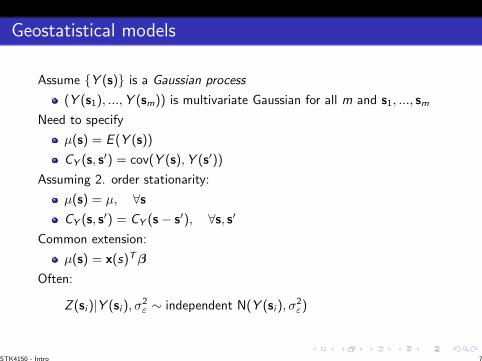
Geostatistical models
Assume {Y (s)} is a Gaussian process
(Y (s1), ...,Y (sm)) is multivariate Gaussian for all m and s1, ..., sm
Need to specify
µ(s) = E (Y (s))
CY (s, s′) = cov(Y (s),Y (s′))
Assuming 2. order stationarity:
µ(s) = µ, ∀sCY (s, s′) = CY (s− s′), ∀s, s′
Common extension:
µ(s) = x(s)Tβ
Often:
Z (si )|Y (si ), σ2ε ∼ independent N(Y (si ), σ
2ε)
STK4150 - Intro 7

Covariance function and Variogram
Dependence can be specified through covariance functions or theVariogram
2γY (h) ≡var[Y (s + h)− Y (s)]
=var[Y (s + h)] + var[Y (s)]− 2cov[Y (s + h),Y (s)]
=2CY (0)− 2CY (h)
Variograms are more general than covariance functions
Variogram can exist even if var[Y (s)] =∞!
In variograms relative changes are modelled model rather than theprocess it self.
In Geostatistics it is common to use variograms.
All formulas ”Covariance formulas” have corresponding ”Variogramformulas”.
γY (h) sometimes called semi-variogram
STK4150 - Intro 8

Stationary, isotropic, anisotropic
Strong stationarity For any (s1, ..., sm) and any h
[Y (s1), ...,Y (sm)] = [Y (s1 + h), ...,Y (sm + h)]
Stationarity in meanE(Y (s)) = µ, for all s ∈ DA
Stationarity covariance (Depend only on lag )cov(Y (s),Y (s + h)) = CY (h), for all s, s + h ∈ DA
Isotropic covariance (depend only on length of lag)cov(Y (s),Y (s + h)) = CY (‖h‖) for all s, s + h ∈ DA
Geometric anisotropy in covariance (”Rotated coordinate system”)cov(Y (s),Y (s + h)) = CY (‖Ah‖), for all s, s + h ∈ DA
Weak stationarity : Stationarity in mean and a stationarity covariance.(recall time series)
STK4150 - Intro 9

Isotropic covariance functions/variograms
Matern covariance function
CY (h;θ) = σ21{2θ2−1Γ(θ2)}−1{||h||/θ1}θ2Kθ2(||h||/θ1)
Powered-exponential
CY (h;θ) = σ21 exp{−(||h||/θ1)θ2}
Exponential
CY (h;θ) = σ21 exp{−(||h||/θ1)}
Gaussian
CY (h;θ) = σ21 exp{−(||h||/θ1)2}
Note:Many different ways to define the ”Range parameter” θ1.e.g. σ2
1 exp{−3(||h||/R)ν}
STK4150 - Intro 10

Stationary spatial covariance functions
STK4150 - Intro 11

Simulation of stationary spatial random field
STK4150 - Intro 12

Isotropic Covariance
Benefit of isotropic assumption is that we only need 1D functions
Note: not all covariance functions / variograms valid in 1D are valid asisotropic covariance functions in higher dimensions.
STK4150 - Intro 13

Bochner’s theorem
A covariance function needs to be positive definite
Theorem (Bochner, 1955)
If∫∞−∞ · · ·
∫∞−∞ |CY (h)|dh <∞, then a valid real-valued covariance
function can be written as
CY (h) =
∫ ∞−∞· · ·∫ ∞−∞
cos(ωTh)fY (ω)dω
where fY (ω) ≥ 0 is symmetric about ω = 0.
fY (ω): Spectral density of CY (h).
STK4150 - Intro 14

Nugget effect and Sill
We have
CZ (h) =cov[Z (s),Z (s + h)]
=cov[Y (s) + ε(s),Y (s + h) + ε(s + h)]
=cov[Y (s),Y (s + h)] + cov[ε(s), ε(s + h)]
=CY (h) + σ2εI (h = 0)
Assume
CY (0) =σ2Y
limh→0
[CY (0)− CY (h)] =0
Then
CZ (0) = σ2Y + σ2
ε Sill
limh→0
[CZ (0)− CZ (h)] = σ2ε = c0 Nugget effect
Possible to include nugget effect also in Y -process.STK4150 - Intro 15

Nugget/sill
STK4150 - Intro 16

Nugget/sill
Sill is a fixed finite level which the variogram converges towards atlarge lag (i.e. ‖h‖ → ∞).
Variograms without a sill (γ(h)→∞ as ‖h‖ → ∞) has noequivalent correlation function.
The nugget effect is variability below the resolution in our model.
In the setting with point observations, i.e. Zi = Y (si ) + εi it isdifficult (often impossible) to distinguish nugget effect in randomfield Y (si ) and observation error εi . This becomes a modellingchoice.
Some softwares mixes nugget effect and observation error.
STK4150 - Intro 17

Estimation of variogram/covariance function
2γZ (h) ≡var[Z (s + h)− Z (s)]
Const expectation= E [Z (s + h)− Z (s)]2
Can estimate from “all” pairs having distance h between.Problem: Few/no pairs for all hSimplifications
Isotropic: γZ (h) = γ0Z (||h||)Lag bin: 2γ0Z (h) = ave{(Z (si )− Z (sj))2; ||si − sj || ∈ T (h)}If covariates, use residuals
STK4150 - Intro 18

Boreality data
Empirical variogram: Boreality data
STK4150 - Intro 19

Testing for independence
If independence: γ0Z (h) = σ2Z
Test-statistic F = γZ (h1)/σ2Z , h1 smallest observed distance
Reject H0 for |F − 1| largePermutation test: Keep spatial positions, and keep values of residuals,but scramble the pairing, i.e. reassign residuals to new spatial positions.Recalculate F for all permutations of Z (or for a random sample ofpermutations)If observed F is above 97.5% percentile, reject H0
Boreality example:
P-value = 0.0001STK4150 - Intro 20

Prediction in multivariate Gaussian models
(Z (s1), ...,Z (sm),Y (s0)) is multivariate GaussianCan use rules about conditional distributions:(
X1
X2
)∼MVN
((µ1
µ2
),
(Σ11 Σ12
Σ21 Σ22
))E (X1|X2) =µ1 + Σ12Σ−122 (X2 − µ2)
var(X1|X2) =Σ11 −Σ12Σ−122 Σ21
Need
Expectations: As for ordinary linear regression
Covariances: New!
STK4150 - Intro 21

Prediction in the spatial model
(Y (s0)
Z
)∼MVN
((µ(s0)µZ
),
(CY (s0, s0) c(s0)
c(s0)T CZ
))c(s0) =cov[Z,Y (s0)]
=cov[Y,Y (s0)]
=(CY (s0, s1), ...,CY (s0, sm))
=cY (s0)
CZ ={CZ (si , sj)}
CZ (si , sj) =
{CY (si , si ) + σ2
ε, si = sj
CY (si , sj), si 6= sj
E(Y (s0)|Z) = µ(s0) + c(s0)TC−1Z (Z − µZ )
Var(Y (s0)|Z) = CY (s0, s0)− c(s0)TC−1Z c(s0)
STK4150 - Intro 22

Kriging = Prediction
Model
Y (s) =x(s)Tβ + δ(s)
Zi =Y (si ) + εi
Prediction of Y (s0), i.e. in an unobserved location.Linear predictors {LTZ + k}Optimal predictor minimize
MSPE(L, k) ≡E [Y (s0)− LTZ− k]2
=var[Y (s0)− LTZ− k] + {E [Y (s0)− LTZ− k]}2
Note: Do not make any distributional assumptions
STK4150 - Intro 23

Kriging
MSPE(L, k) =var[Y (s0)− LTZ− k] + {E [Y (s0)− LTZ− k]}2
=var[Y (s0)− LTZ− k] + {µY (s0)− LTµz − k]}2
Second term is zero if k = µY (s0)− LTµZ .First term (c(s0) = cov[Z,Y (s0)]):
var[Y (s0)− LTZ− k] =CY (s0, s0)− 2LTc(s0) + LTCZL
Derivative wrt LT :
− 2c(s0) + 2CZL = 0
L∗ = C−1Z c(s0)
giving
Y ∗(s0) =µY (s0) + c(s0)TC−1Z [Z− µZ ]
MSPE(L∗, k∗) =CY (s0, s0)− c(s0)TC−1Z c(s0)
STK4150 - Intro 24

Kriging (Simple Kriging)
The Kriging predictions with a known mean is:
c(s0) =cov[Z,Y (s0)]
=cov[Y,Y (s0)]
=(CY (s0, s1), ...,CY (s0, sm))
=cY (s0)
CZ ={CZ (si , sj)}
CZ (si , sj) =
{CY (si , si ) + σ2
ε, si = sj
CY (si , sj), si 6= sj
Y ∗(s0) = µY (s0) + cY (s0)TC−1Z (Z− µZ )
STK4150 - Intro 25

Gaussian assumptions
Recall now Y,Z are MVN(Z
Y(s0)
)= MVN
((µZ
µY (s0)
),
(CZ cY (s0)T
cY (s0) CY (s0, s0)
))Give
Y (s0)|Z ∼ N(µY (s0) + c(s0)TC−1Z [Z− µZ ],CY (s0, s0)− c(s0)TC−1Z c(s0))
Same as kriging!The book derive this directly without using the formula for conditionaldistribution
STK4150 - Intro 26

Compare to interpolation
Assume no observation error
Consider deviations from µ(s) ,i.e. f (s) = Y (s)− µ(s).
Set fi (s) = CY (s− si )
Then:
F = CZ (= CY no observation error)
(FTF)−1FT = C−1Z (symmetry)
β = C−1Z Z
f (s0) =∑n
i=1 βiCY (s0 − si )
Which gives the same result again:
f (s0) = βTc(s0) = (ZT )C−1Z c(s0)
Y ∗(s0) = µ(s0) + c(s0)TC−1Z (Z− µZ) If we include µ(s) we get
STK4150 - Intro 27

Spatial prediction comments
Given the mean and covariance function Kriging and the a Gaussianrandom field model give identical spatial correlations.There are stronger assumptions underlying the Gaussian model thanneeded in KrigingKriging is the optimal linear predictor for any distribution (not onlygaussian)For the Gaussian model the linear prediction is optimal (among all),for other distributions there might be other predictors which arebetter.The Gaussian model is easier to extend using a Hierarchical approachIn Kriging and Gaussian random field, ”interpolating functions” aredetermined by dataIn Kriging it is common to use plugin estimate for the covariancefunctionThe hierarchical approach is suited to include uncertainty on modelparametrers.the Mean Squared Prediction Error (MSPE) is used for both Krigingand hierarchical model (HM)
STK4150 - Intro 28

So fa and Next:
Simple kriging
Linear predictorAssume parameters knownEqual to conditional expectation
Unknown parameters
Ordinary krigingPlug-in estimatesBayesian approach
Non-Gaussian models
STK4150 - Intro 29

So fa and Next:
Simple kriging
Linear predictorAssume parameters knownEqual to conditional expectation
Unknown parameters
Ordinary krigingPlug-in estimatesBayesian approach
Non-Gaussian models
STK4150 - Intro 30

Unknown parameters
So far assumed parameters known, what if unknown?
Direct approach -Universal and Ordinary kriging (for meanparameters)
Plug-in estimate/Empirical Bayes
Bayesian approach
STK4150 - Intro 31

Kriging (cont)
Y ∗(s0) = µY (s0) + cY (s0)TC−1Z (Z− µZ )
Assuming
E [Y (s)] =x(s)Tβ
Z (si )|Y (si ), σ2ε ∼ind.Gau(Y (si ), σ
2ε)
Then
µZ =µY = Xβ
CZ =ΣY + σ2εI
cY (s0) =(CY (s0, s1), ...,CY (s0, sm))T
and
Y ∗(s0) = x(s0)β + cY (s0)T [ΣY + σ2εI]−1(Z− Xβ)
STK4150 - Intro 32

Kriging
Simple kriging, EY (s) = x(s)Tβ, known
Y ∗(s0) = x(s0)β + cY (s0)TC−1Z (Z− Xβ)
Universal kriging, EY (s) = x(s)Tβ, unknown
Y (s0) =x(s0)T βgls + cY (s0)TC−1Z (Z− Xβgls)
βgls =[XTC−1Z X]−1XTC−1z Z
Bayesian kriging, EY (s) = x(s)Tβ, with β ∼ N(β0,Σ0)
Y (s0) =x(s0)T βB + cY (s0)TC−1Z (Z− XβB)
βB =β0 + Σ0XT (XΣ0XT + CZ )−1(Z− Xβ0)
Possible to show the SK and UK are the limiting cases of BKΣ0 → 0⇒ BK → SKΣ0 →∞⇒ BK → UK
STK4150 - Intro 33

Kriging
Simple kriging, EY (s) = x(s)Tβ, known
Y ∗(s0) = x(s0)β + cY (s0)TC−1Z (Z− Xβ)
Universal kriging, EY (s) = x(s)Tβ, unknown
Y (s0) =x(s0)T βgls + cY (s0)TC−1Z (Z− Xβgls)
βgls =[XTC−1Z X]−1XTC−1z Z
Bayesian kriging, EY (s) = x(s)Tβ, with β ∼ N(β0,Σ0)
Y (s0) =x(s0)T βB + cY (s0)TC−1Z (Z− XβB)
βB =β0 + Σ0XT (XΣ0XT + CZ )−1(Z− Xβ0)
Possible to show the SK and UK are the limiting cases of BKΣ0 → 0⇒ BK → SKΣ0 →∞⇒ BK → UK
STK4150 - Intro 34

Kriging
Simple kriging, EY (s) = x(s)Tβ, known
Y ∗(s0) = x(s0)β + cY (s0)TC−1Z (Z− Xβ)
Universal kriging, EY (s) = x(s)Tβ, unknown
Y (s0) =x(s0)T βgls + cY (s0)TC−1Z (Z− Xβgls)
βgls =[XTC−1Z X]−1XTC−1z Z
Bayesian kriging, EY (s) = x(s)Tβ, with β ∼ N(β0,Σ0)
Y (s0) =x(s0)T βB + cY (s0)TC−1Z (Z− XβB)
βB =β0 + Σ0XT (XΣ0XT + CZ )−1(Z− Xβ0)
Possible to show the SK and UK are the limiting cases of BKΣ0 → 0⇒ BK → SKΣ0 →∞⇒ BK → UK
STK4150 - Intro 35

Ordinary kriging
Ordinary kriging, EY (s) = µ, unknown (special case of UK)
Y (s0) ={cY (s0) +1(1− 1TCZ−1cy (s0))
1TC−1Z 1}TC−1Z Z
=µgls + cY (s0)TC−1Z (Z− 1µgls)
µgls =[1TC−1Z 1]−11TC−1z Z
To minimize the MSPE, we make an unbiased estimate with theminimum variance.
MSPE(λ) = E (Y (s0)− λTZ)2
Unbiased constraint:
E [Y (s0)]− E [λTZ] = 0
Prediction variance:
PV (λ) = CY (s0, s0)− 2λT cY (s0) + λTCZλ
STK4150 - Intro 36

Ordinary kriging equations
We have: E [Y (s0)] = µ and E [λTZ] = λTE [Z] = λT1µ thus
µ = λT1µ⇒ 1 = λT1
The problem then becomes:
minλ
PV (λ)
subject to:1 = λT1
Solved by Lagrange multiplier, i.e. minimize
CY (s0, s0)− 2λT cY (s0) + λTCZλ− 2κ(λT1− 1)
Differentiation wrt λT gives (which is combined to the final resultpresented on previous page):
−2cY (s0) + 2CZλ =2κ1
λT1 =1
STK4150 - Intro 37